| Issue |
A&A
Volume 697, May 2025
|
|
|---|---|---|
| Article Number | A138 | |
| Number of page(s) | 22 | |
| Section | Astrophysical processes | |
| DOI | https://doi.org/10.1051/0004-6361/202452549 | |
| Published online | 14 May 2025 | |
Impact of active galactic nucleus feedback modes on the turbulent properties of the multiphase intracluster medium
1
Dipartimento di Fisica e Astronomia, Università di Bologna, Via Gobetti 93/2, 40129 Bologna, Italy
2
INAF – Osservatorio di Astrofisica e Scienza dello Spazio di Bologna, Via Gobetti 93/3, 40129 Bologna, Italy
3
Istituto di Radio Astronomia, INAF, Via Gobetti 101, 40129 Bologna, Italy
4
University of California Observatories/Lick Observatory, Department of Astronomy and Astrophysics, Santa Cruz, CA 95064, USA
⋆ Corresponding author: This email address is being protected from spambots. You need JavaScript enabled to view it.
Received:
9
October
2024
Accepted:
25
February
2025
Abstract
The feedback from active galactic nuclei (AGN) plays a crucial role in regulating the thermodynamics and the dynamics of the intracluster medium (ICM). Studying the turbulent patterns of the hot and warm ionized phases may allow us to determine how these phases are involved in the AGN cycle and the amount of turbulent pressure generated by the latter. For this work we used new simulations to study the turbulent motions created by different types of AGN feedback in a cool core cluster and to predict the observable signatures with the latest X-ray telescopes (e.g., XRISM). We ran several hydrodynamic simulations with ENZO, simulating the self-regulated cycles of AGN feedback, starting from a static ICM in a cluster that represents the Perseus cluster. We studied in detail different feedback modes, from pure kinetic precessing jets to almost pure thermal feedback. Our analysis reveals that the gas velocity dispersion in the center of the cluster correlates in time with the peaks of the AGN activity. In more than 50% of the cluster evolution different feedback modalities produce the velocity dispersion observed in the Perseus cluster, while leading to distinct geometrical distributions and velocity dispersion profiles. Moreover, we do not find a significant kinematic coupling between the hot and the cold phase kinematics. We find a correlation between the AGN activity and the steepening of the velocity structure function (VSF) and that the projected 2D VSF slopes are not trivially correlated with the 3D VSF slopes. This line of research will allow us to use incoming detections of gas turbulent motions detectable by XRISM (or future instruments) to better constrain the duty cycle, energetics, and energy dissipation modalities of AGN feedback in massive clusters of galaxies.
Key words: galaxies: active / galaxies: clusters: general / galaxies: clusters: intracluster medium / galaxies: jets
© The Authors 2025
 Open Access article, published by EDP Sciences, under the terms of the Creative Commons Attribution License (https://creativecommons.org/licenses/by/4.0), which permits unrestricted use, distribution, and reproduction in any medium, provided the original work is properly cited.
This article is published in open access under the Subscribe to Open model. This email address is being protected from spambots. You need JavaScript enabled to view it. to support open access publication.
1. Introduction
Cool-core clusters of galaxies are objects that are believed not to have undergone major merger events in the recent past. Their intracluster medium (ICM) in the central region is characterized by a positive temperature gradient and a relatively short cooling time (≲a few gigayears). The gas entropy profiles increase toward the external regions, and show a low-entropy core with values around 10 − 50 KeV cm2 (e.g., Fabian 1994; Hudson et al. 2010; Sanders et al. 2010).
The (thermo)dynamics of these objects is believed to be self-regulated by the interplay of radiative gas cooling (causing overall inward gas motions of the external gas layers around the core), and feedback events by the central active galactic nucleus (AGN) located in the central galaxy at the bottom of the cluster potential well, triggered by the accretion of matter onto the central supermassive black hole (SMBH; for a review see Fabian 2012). The description of the ICM still poses formidable open problems to the theory that can be constrained by knowing the turbulent structure of the gas: hydrostatic bias, in other words the masses obtained considering a hydrostatic equilibrium are underestimated with respect to those computed by gravitational lensing, suggesting the presence of other contributions to the pressure support in addition to the thermal pressure (Eckert et al. 2019); the distribution of metals (i.e., how the turbulence diffuses and affects the metal profile in the ICM (Simionescu et al. 2008; Werner et al. 2010); and thermal heating due to the turbulence dissipation of the central AGN (Yang & Reynolds 2016; Bourne & Sijacki 2021; Zhuravleva et al. 2014). In a cool core cluster, there are several sources of turbulence in the ICM: cluster galaxy motions throughout the cluster; cosmological accretion or minor mergers occurring at the borders in the external regions (Vazza et al. 2011); sloshing and AGN activity in the central regions (Vazza et al. 2012; Heinz et al. 2010; Randall et al. 2015; Yang & Reynolds 2016; Lau et al. 2017; Bourne & Sijacki 2017; Bourne et al. 2019).
The AGN activity of the central SMBH is certainly a key process that affects the cluster in many ways. First of all, as mentioned above, AGN feedback is thought to be the engine that regulates the thermodynamics of the cluster, heating the ICM but maintaining the cool core in a self-regulated way. As suggested, the feeding of the AGN is due to the cold gas that reaches the proximity of the SMBH (Pizzolato & Soker 2005, 2010; Soker 2006; Gaspari et al. 2012; Gaspari & Churazov 2013; Werner et al. 2014; Voit et al. 2015). The cold gas is observed at the center of galaxy clusters appearing as atomic and molecular phases (Conselice et al. 2001; Babyk et al. 2019; Olivares et al. 2019; Gingras et al. 2024). It extends in regions of typical size of 10 − 70 kpc for the atomic phase and 10 − 20 kpc for the molecular phase. It often appears with filamentary and clumpy shapes (Olivares et al. 2019). The size of the clumps is likely smaller than ∼70 pc since the clumps are not resolved even with the highest resolutions (Conselice et al. 2001; Olivares et al. 2019). The link between the AGN activity and the cold gas formation has been debated and is still not totally clear, but theories and simulations have made significant progress on this topic (McNamara et al. 2016; Voit et al. 2017; Gaspari et al. 2018). The jets generated by the AGN are thought to be both heat sources and catalysts of the cold gas formation: as the jets move through the ICM, they entrain hot gas from the center and the turbulence present at the edges of the jets helps the mixing of the layers and makes the cooling time shorter, favoring the condensation of the gas in clumps. Then, moved by gravity and losing angular momentum through several processes, the clumps fall toward the cluster center and the SMBH. This process has been reproduced in several simulations (Gaspari et al. 2011a,b; Li & Bryan 2014a; Li et al. 2015; Beckmann et al. 2019; Wang et al. 2021). The study of the hot and cold gas motion and the link between them helps us to better understand the feeding and the heating of the AGN cycle.
The velocity structure function (VSF) is a tool for analyzing the properties of turbulence. VSFs of the cold phase have been calculated in many systems (e.g., Li et al. 2020, 2023; Ganguly et al. 2023; Gingras et al. 2024). However, due to the limitations of the current X-ray telescopes, accurate VSFs of the hot ICM are generally not available yet (but see Gatuzz et al. 2023 for current constraints using XMM-Newton EPIC data). Forthcoming XRISM observations are expected to greatly boost our understanding of hot gas kinematics.
Simulations of kinetic mode feedback with different implementations have shown that this feedback mode is capable of producing a level of turbulence observed at cluster center (Bourne & Sijacki 2017; Ayromlou et al. 2024; Truong et al. 2024). Thermal feedback is also widely used because of its simplicity, even though the presence of kinetic jets is required by observations. It is unclear if purely thermal feedback can capture the basic physical processes at work in cluster centers.
Observations also suggest that precession of radio jets might be common (e.g., Marti-Vidal et al. 2013; Ubertosi et al. 2024). The precession of the SMBH can be due to the Lense–Thirring effect or minor and major mergers of the clusters that end up with the merging of the corresponding SMBHs. In addition, accretion of stars and other episodes of large accretion have been proposed as the origin of radio jet precession.
For this paper we used hydrodynamic simulations of self-regulated AGN heating in cool-core galaxy clusters with different combinations of kinetic and thermal feedback, with and without a precession effect, to study the turbulence created by the different configurations and to check how the hot and cold gas kinematics are affected by these characteristics. By analyzing the gas kinematics through bulk motion and velocity dispersion, and the turbulent properties through the VSF, we were able to constrain the physical properties of the AGN feedback, its efficiency in creating cold gas, and the interactions between this phase and the hot ICM. With the upcoming insights due to the new generation of X-ray telescopes, we will be able to compare the simulation predictions with the real data.
The paper is developed as follows. In Section 2 we explain the initial conditions and the setup of the simulation that is based on Li & Bryan (2014a), and show the runs performed. In Sect. 3 we look briefly at the thermodynamics of evolution to check if the AGN feedback works as a cluster engine. In Section 4 we show in detail the kinematic behavior of the hot and cold phases. In Section 5 we analyze the properties of the turbulence through the use of the VSF. Finally, in Section 6 we discuss the results obtained and give some future prospects.
2. Methods and simulations
In this paper, we adopt the simulation setup and feedback mechanism by Li & Bryan (2012) and Li et al. (2015). Similar procedures have been used in several numerical studies (e.g., Gaspari et al. 2011a,b; Bourne & Sijacki 2017; Wang et al. 2021) and can be considered a state-of-the-art implementation of AGN feedback in single object simulations. Nevertheless, slight differences in the numerical parameters can generate very diverse flows and one of the main objectives of this work is to evaluate the sensitivity of hot and cold gas turbulence on the details of the feedback process. We will explore other feedback techniques in future works.
2.1. Initial conditions
We run our simulations with the ENZO code (enzo-project.org), a cosmological Eulerian code supporting Adaptive mesh refinement, and a large variety of different numerical solvers and physical modules (Bryan et al. 2014). Our simulations start from the numerical setup implemented in a series of works by Li & Bryan and collaborators (Li & Bryan 2012, 2014a,b; Li et al. 2015), which represents a cool core cluster with physical properties based on the Perseus cluster.
We summarize here the fundamental aspects of this model:
-
The static gravitational potential follows the model by Mathews et al. (2006) and is due to an NFW (Navarro et al. 1996) dark matter halo and a central Brightest Cluster Galaxy (BCG), with the following mass distributions:
 (1)
(1)Here y = cr/rvir, c = 6.81 is the concentration, rvir = 2.440 Mpc is the virial radius and Mvir = 8.5 × 10¹⁴ M⊙. The BCG stellar mass distribution is approximated with a fit of a De Vaucouleurs profile with a total mass of 2.43 × 10¹¹ M⊙ and effective radius Re = 6.41 kpc,
![Mathematical equation: $$ \begin{aligned} M_*(r) =\frac{r^2}{G}\Bigg [\Bigg (\frac{r^{0.5975}}{3.206\times 10^{-7}} \Bigg )^s +\Bigg (\frac{r^{1.849}}{1.861\times 10^{-6}} \Bigg )^s \Bigg ]^{-1/s} , \end{aligned} $$](/articles/aa/full_html/2025/05/aa52549-24/aa52549-24-eq2.gif) (2)
(2)in cgs units with s = 0.9 and r in kpc and a central supermassive black hole of MSMBH = 3.4 × 10⁸ M⊙.
-
The initial gas temperature and electron density profiles are fits of X-ray observations of the Perseus cluster (Churazov et al. 2004; Mathews et al. 2006):
 (3)
(3)![Mathematical equation: $$ \begin{aligned} n_{\rm e}(r)&= \frac{0.0192}{1+\big (\frac{r}{18}\big )^3}+\frac{0.046}{\bigg [1+\big (\frac{r}{57}\big )^2\bigg ]^{1.8}}+\frac{0.0048}{\bigg [1+\big (\frac{r}{200}\big )^2\bigg ]^{1.1}}\,\mathrm{cm^{-3}}. \end{aligned} $$](/articles/aa/full_html/2025/05/aa52549-24/aa52549-24-eq4.gif) (4)
(4)These initial conditions represent an ICM in approximate hydrostatic equilibrium in the mass model described above. Therefore, the initial gas velocity is set to zero.
-
The gas loses energy through the cooling function based on Table 4 from Schure et al. (2009). A temperature floor of T = 104 K is set.
-
The simulations start with a root grid of side 64 cells in a comoving box of side L = 16 Mpc, that is redefined by the AMR following criteria in order to resolve denser region, the cooling time and gravitational instability. In particular, a cell is refined when: the gas mass in the cell exceeds 0.2 times the gas mass in a root cell; the cooling time becomes small compared to the crossing time over the cell, in particular when tcool < 6 tcross; the size of the cell is larger than 0.25 of the Jeans length.
More details can be found in Li & Bryan (2012).
By using up to 10 levels of mesh refinement, the highest spatial resolution achieved in our simulations is ≈240 pc.
2.2. Accretion and feedback physics
As stated above, we use a standard implementation of self-regulated AGN feedback. It is built on the long standing idea of cold accretion (e.g., Soker & Pizzolato 2005; Brighenti & Mathews 2003, 2006) onto the central SMBH, which in turn triggers the injection of some form of energy in the surrounding ICM. Both steps must be parametrized in the numerical simulations. This mechanism naturally induces a self-regulated feedback cycle, the features of which, however, critically depend on the numerical details of the implementation. This class of algorithms has been widely used, refined and investigated in the last two decades (just to cite a few Cattaneo & Teyssier 2007; Dubois et al. 2010, 2011; Gaspari et al. 2011a,b, 2012; Li & Bryan 2014a,b; Li et al. 2015; Yang & Reynolds 2016; Cielo et al. 2017; Bourne & Sijacki 2017, 2021, for a review see Bourne & Yang 2023).
The energy injection depends on the accretion rate, which is controlled by the quantity of the cold gas near the SMBH. More specifically, the gas is accreted when the following conditions are fulfilled:
-
the gas has to be colder than a threshold temperature Tthres = 3 × 10⁴ K,
-
the gas must be within a cubical region of side 1 kpc around the SMBH. This is called the accretion region.
-
the mass of cold gas in the accretion region must be larger than a threshold value, Mthres = 107 M⊙.
When a quantity of cold gas Macc satisfied these conditions, the accretion rate onto the SMBH is estimated as Ṁ = Macc/τ, where τ = 5 Myr roughly represents the free fall time in the accretion region.
The total power in the jet is
 (5)
(5)
where c is the light velocity and ϵ = 10−3 is the effective accretion efficiency. To generate the jets, a quantity of mass (and energy, see below) is added on two planes parallel to the equatorial plane, at a height on the z-axis hjet = 2 kpc. The amount Δm added in each cell of the planes is calculated so that ΣΔm = ṀΔt and Δm ∝ exp−r2/2rjet2, with r being the distance from the z-axis and rjet = 1.5 kpc.
Needless to say, in reality some fraction Ṁ would accrete onto the black hole and disappear from the flow. Thus, a simplifying assumption here is to neglect the black hole growth and assume that Ṁ = Ṁjet (i.e., the entire accreted mass gas is deposited in the jet region).
The AGN energy (and power) can be injected either in kinetic or thermal form in the jet launching region. This is regulated by the parameter fkin, which sets the fraction of the total feedback power converted into jet kinetic power, Ėkin = fkinPjet. We see that predominantly thermal feedback (small fkin) or predominantly kinetic feedback (large fkin) leads to quite different flows. The launching velocity of jets thus depends on the kinetic fraction fkin, vjet2 = 2fkinϵc2, through the formula  . In the jet launching planes, the momentum of each cell is vjetΔm, and the final velocity of each cell is computed considering that the total momentum is conserved. When there is no thermal feedback, in the jet launching bases where the gas mass is added, the temperature is lowered in order to keep the thermal energy of the cell constant. A side effect of this choice is an artificial decrease of the local cooling time, which favors cold clumps formation, as we show in the discussion. When there is predominantly thermal feedback, energy is directly injected as thermal energy, by adding to each cell of the jet launching region the quantity (1 − fkin)Δmϵc2. In this paper, we explore a range of the parameter fkin to investigate its impact on the feedback modes. We also consider the possibility of jet precession along the z-axis. The jet has an precession angle of θp ≈ 9°, and a period of τp = 10 Myr.
2.3. Runs
In order to investigate the differences in the feedback modes and the effect of jet precession we have performed six independent hydrodynamic simulations. In detail, the three feedback modes explored here are:
-
K1np, the feedback is purely kinetic (fkin = 1) and there is no jet precession. The model K1 is similar, but precession is present.
-
K05np, a mixed thermal and kinetic feedback modality, in which fkin = 0.5. Model K05 has also fkin = 0.5 but includes jet precession.
-
K01np, a predominantly thermal feedback model, fkin = 0.1, without precession. Similarly, model K01 has fkin = 0.1 and precession.
We complement these feedback simulations with an extra run in which there is no feedback whatsoever, CF, with the feedback switched off for the entire evolution of the cluster and a classical cooling flow develops.
In the next section, we analyze the thermodynamic evolution of the ICM and the observable radial profiles in the various models, before analyzing in detail the ICM kinematic. Since the AGN cycle is self-regulated and the feedback modes are different, soon after the begin of the feedback stage we observe significantly different feedback and cooling evolution.
3. Results: Thermodynamic evolution
Here, we present maps and profiles of the most relevant thermodynamical quantities. This analysis is straightforward but essential to establish if the simulated clusters agree with the basic X-ray observations. It is notoriously problematic, for heated flows, to satisfy at the same time the tight constraints on the cooling rate and having acceptable temperature and density profiles. This can be considered the first test that any realistic AGN feedback model must pass. See, for instance, the discussions in Brighenti & Mathews (2002, 2003, 2006) and in Gaspari et al. (2011a,b)
The six panels of Fig. 1 show the temperature and density of the central slice around the plane y = 0 of the six runs. For each model, we display representative snapshots near the peak of activity of each AGN model. By simple visual inspection, a few salient features can be identified of our feedback implementations, also described below in a more quantitative way. The highest amount of perturbation in the ICM is observed in the purely kinetic feedback model K1, followed by the hybrid kinetic and thermal feedback without precession K05np and finally by the two almost purely thermal with and without precession runs, K01 and K01np. A distinctive and potentially observable feature is the persisting presence of very elongated cavities, or tunnels, along the jet direction. We also note (see Fig. 9) that in the purely kinetic run, the amount of the accreted or long-lived cold gas is larger than in K05np run and the purely thermal cases K01 and K01np. This suggests a close connection between the level of disturbance or turbulence of the hot ICM and the presence of inhomogeneities prone to thermal instability (e.g., Gaspari et al. 2012, 2013).
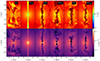 |
Fig. 1. Gas temperature (top) and density (bottom) maps in the x − z plane of the K1, K1np, K05, K05np, K01, and K01np runs (from left to right). The images are not taken at the same absolute time, but rather at the epoch of the maximum AGN feedback power in each run. Movies for the precessing jet simulations can be watched at https://www.youtube.com/watch?v = 7HgSL4xY8lI, https://www.youtube.com/watch?v = 9_SnQm5R8Vs, and online |
At variance with the previous models is run K05, which forms a long-lasting cold gas disk that leads the system to an accretion and feedback power almost constant with time, leaving the ICM less perturbed. Finally, the purely kinetic run without precession K1np soon runs into an unrealistic trend, creating two thin, relatively dense jets able to escape the cluster itself. They do not efficiently heat the cluster core and are also incompatible with observations (e.g., Fabian 2012). Such straight and X-ray bright features have never been observed in X-rays, and assuming that jets should also be filled with relativistic plasma, they would produce radio emission features incompatible with radio sources in clusters. We remark that this result is a consequence of the assumed accretion scheme, which generates a continuous accretion. This implies that the (not precessing and purely kinetic) jets mostly interact with a relatively smooth and unperturbed ICM, frequently generating new shocks and cavities. This underlines once more the impact of the numerical schemes on the simulated feedback physics. It should be noticed that other schemes in the literature, like those used in Gaspari et al. (2011a,b), result in a more bursty AGN activity.
In the following, we study the thermodynamic profiles of the ICM in order to test our models against X-ray observations, in a statistical sense. In particular, we want to check which run is able to prevent the catastrophic cooling of gas in the cluster core and, at the same time, to maintain a quasi-steady balance between cooling and heating, preserving the cluster cool core. We first analyze the different accretion and power histories of each run, and compare their various thermodynamic radial profiles with X-ray observations of real clusters, in a similar mass range of our simulated Perseus cluster.
Figure 2 shows the evolving feedback power recorded in all runs, as well as their total time-integrated feedback energy. In our simulations, and as already found in many others (e.g., Brighenti & Mathews 2002; Revaz et al. 2008; Gaspari et al. 2011b; Li & Bryan 2014a; Qiu et al. 2020), cold clumps often form in the outflows, out of the condensation of overdense material formed near the jet, and then fall back into the black hole. This circulation leads to a frequent feeding of the black hole over short periods. This can generate both strong, sparse AGN outbursts or a more continuous, smooth SMBH activity. Both regimes are allowed by the broad scenario of the chaotic cold accretion (CCA; e.g., Gaspari et al. 2011a,b).
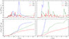 |
Fig. 2. Evolution of the jet feedback power (top) and integrated power (bottom) for the three runs with jet precession (right) K1 (blue dot-dashed), K05 (green dashed), and K01 (red solid), and without precession (left) with the same color and line-coding. |
Different feedback modes heat the gas in the central region with different efficiency, and the additional presence of jet precession further affects the net heating of the cluster core, as well as the long term history of the injected feedback power. In particular, even though runs K1 and K05np inject energy in the ICM in a different way, kinetic the former and kinetic and thermal the latter, they end up with similar quantity of cold gas accreted and thus similar power histories up to t ∼ 3 Gyr, when they experience a maximum power of 1.5 × 1046 erg/s. However, while in model K1 the AGN drops smoothly afterward, in model K05np the AGN activity proceeds with a bursty regime, with several power peaks of about 4 × 1045 erg/s. The latter behavior is explained by the absence of precession, which facilitates the arrival of cold gas in the accretion region, while the former is due to the higher efficiency in creating dense cold gas clumps. Run K05 has a lower and remarkably smoother power history. In this case, the formation of a cold disk leads to an almost constant accretion rate and a steady feedback power. Runs K01np and K01 show very similar trends, as expected, considering that the only difference is in the precession of kinetic jets, which however only account for a 10% of the total feedback power. They both have a lower, albeit irregular, history of feedback power, resulting in a total feedback energy lower than in the other cases (i.e. 6 × 1061 erg).
The time integrated power for all the simulated models does not exhibit large differences, being limited in the range 7 − 15 × 1061 erg (at t = 6 Gyr), with the thermal models K01 and K01np being a factor of 2 less energetic than the kinetic runs. The only exception is model K1np, which produces two thin and continuous jets which are unable to heat the gas in the cluster core. The jet power and energy quickly reach extreme values, but the heating is released at ∼1 Mpc from the center. This peculiar evolution, which sometimes happens for purely kinetic, non-precessing narrow jets, causes a very non-isotropic – and so not efficient – ICM heating (e.g., Vernaleo & Reynolds 2006). As a counterexamples, the jets in Brighenti & Mathews (2006) or in Gaspari et al. (2011a,b), triggered in a more intermittent way, are able to distribute the heat in a wide volume.
We now compare the simulated radial temperature, density and entropy profiles with the observed profiles in cool core clusters within the mass range of our simulated Perseus cluster, taken from the X-ray ACCEPT sample by Cavagnolo et al. (2009). Figure A.1 (see Fig. 3 for an example) shows the density, the emission weighted temperature and the derived entropy profiles of some snapshots of our runs, overplotted on the observed ones from Cavagnolo et al. (2009). Only the region r > 10 kpc is meaningful, since the inner zone is largely affected by the numerical implementation of the feedback mechanism. We can see that for most outputs the profiles of our runs are in the same range as values of the observed one, except for run K1np for which the temperature and density profiles fail in the central 100 kpc size region. Notably, in all models, the drop in the central temperature, a signature of a cool core cluster, is preserved.
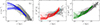 |
Fig. 3. Gas density (left), X-ray emission weighted temperature (center), and entropy radial profiles (left) obtained at several epochs during the cluster evolution in run K1. The comparison with the other runs is shown in Fig. A.1. The additional gray lines show the distribution of corresponding profiles obtained from the ACCEPT sample by Cavagnolo et al. (2009) for clusters with a central temperature in a range of 3 ≤ T ≤ 5 KeV and a central entropy less than 50 KeV/cm2 meant to select cool core cluster with masses close to the simulated Perseus-like cluster. |
The simulations last roughly 6 Gyr, a long time during which real clusters evolve through cosmological processes like accretion and merging. Our isolated cluster models neglect the impact of the cosmological evolution, instead focusing on the effect of AGN activity alone. This approximation is justified because Cosmic accretion on the outskirts of the clusters mostly affects the outer structure and its mass profile and less the physical properties of the (relaxed) cores. These are mostly controlled by internal processes, such as cooling and AGN feedback1.
To summarize this section, we conclude that all runs, excluding K1np, are able to maintain, at least at first order, a balance between cooling and heating without breaking the cool core temperature profile. Therefore, we move to the kinematic analysis of the five survived models in the next sections.
4. Results: Kinematic ICM analysis
To study the kinematic and turbulent properties of the ICM, we split the analysis into two components:
-
the hot phase: all the gas emitting X-ray radiation (i.e., cells with a temperature above T = 106 K). For the 2D projections, to compare our data with observations we weigh the velocities by the emissivity of the cell. The emission weighted i-component of the velocity is
 (6)
(6)where the integration is performed along the line of sight (LOS) in the i-direction and N is the number of cells along the LOS specified at each computation.
-
the cold phase: all the cells with a temperature below T = 5 × 10⁴ K. This gas phase is usually observed near the cluster center, through emission lines (e.g., Hα, [OII]). The projected velocities of cold gas are computed by taking a constant value of the cooling emission for the Hα line (case B recombination, T = 104 K) ΛHα = 3.3 × 10⁻²⁵ [cgs] (Osterbrock & Ferland 2006):
 (7)
(7)
For simplicity, we assume that there is neither neutral or molecular gas nor dust in the cold phase, which is optically thin, even if this assumption is unlikely to be realistic.
In the following, we solve the two sums along the LOS of our observations, for different volume selections which are specified from case to case.
4.1. Hot phase
4.1.1. Kinematical maps and σ profiles
We start by studying the kinematics of the hot gas phase by calculating quantities observable (or potentially observable) in X-rays. We focus first on model K1 and then briefly discuss the other runs. We recall that in our simulations the ICM is set initially completely at rest (i.e., no rotation or random motion is set in the initial condition). At first, a classic cooling flow stage sets in, with timescale tcool ≈ 1 Gyr, during which the gas starts flowing toward the center with average velocities on the order of ≃10 km/s. When the feedback gets activated, the gas along the jet axis begins to experience strong accelerations. The first two top rows of Fig. 4 show the temperature in the meridional plane (first panel) and the X-ray emission weighted projected velocity along the x-axis, a LOS perpendicular to the jets (second panel) at three different epochs of run K1, with the time increasing from left to right. In the same way, the first two rows of Fig. 5 show a temperature map on a plane defined by z = 100 kpc and the X-ray emission weighted z-component of the velocity, vz, projected along the z-axis (that is, the jet axis).
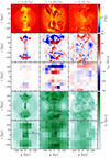 |
Fig. 4. Quantities listed in the following at three epochs (from left to right: t = 2.16, 3.29, and 5.25 Gyr) of the kinetic run with precession K1. Top panels: Temperature field in the meridional plane. Second and fourth panels: X-ray emission weighted projected velocity map and corresponding velocity dispersion obtained using Eqs. (6) and (8) along a LOS perpendicular to the jet axis. Third and fifth panels: grained X-ray emission weighted projected velocity and velocity dispersion maps obtained from Eqs. (9) and (10) using a pixel of 30 × 30 kpc along the same LOS perpendicular to the jet axis. |
 |
Fig. 5. Several quantities at three epochs (from left to right: t = 2.16, 3.29, and 5.25 Gyr) of the kinetic run with precession K1. Top panels: Temperature field in a plane perpendicular to the jet axis at 100 kpc from the center. Second and fourth panels: X-ray emission weighted projected velocity map and corresponding velocity dispersion obtained using Eqs. (6) and (8) along the LOS parallel to the jet axis. Third and fifth panels: Grained X-ray emission weighted projected velocity and velocity dispersion maps obtained from Eqs. (9) and (10) using a pixel of 30 × 30 kpc along the LOS parallel to the jet axis. |
During the first episodes of AGN feedback (t = 2.16 Gyr in the images), the jets pierce the ICM and start to expand laterally, at a height z ≃ 100 kpc. The jet material mixes with the ICM through dynamical instabilities at the jet edges, yet the motion of the gas is mainly confined within the cone traced by the precession of jets. The first velocity maps (first epoch of Figs. 4 and 5) allow us to approximately trace this cone. At later times (t = 3.29 Gyr), the AGN has produced several outbursts and we are close to the peak of the feedback power. Jets have inflated hot and underdense bubbles, which in turn set in motion the gas at a larger lateral distance from the jet cone (as shown in the second epoch of Figs. 4 and 5). Later on, after ≈4 Gyr since the first feedback event, gas motions are roughly isotropic and volume filling in the central cluster regions (t = 5.25 Gyr in Figs. 4 and 5).
As AGN feedback can be a key driver of turbulent motions in the core of clusters of galaxies (e.g., Gaspari et al. 2018), we also computed maps of the gas velocity dispersion, projected along the LOS. For example, the velocity dispersion along the x direction is computed as
 (8)
(8)
where the sum is done along the x direction, vp, x is the EW projected velocity in a given point (y, z) on the projection plane, obtained with Eq. (6) and N is the number of cells along the LOS We use a cubic volume of side 300 kpc to perform the computation. In a similar way, σz is computed along the z direction. The fourth row of each epoch in Figs. 4 and 5 show the map of the velocity dispersion along the x and z directions, for model K1.
The velocity dispersion is initially on the order of 102 km/s within the jet cone, and only a few tens of km/s outside the cone, typical of a (slow) cooling flow (left panel). Later on, when the AGN activity is strong, the perturbed region widens, with σx increasing up to ∼450 km/s (central panel). After the strong outbursts and during the period of relatively lower AGN activity, the velocity dispersion stabilizes at values of a few ∼102 km/s. Now σx is more homogeneously distributed in the whole field considered for these projections (300 × 300 kpc2), albeit the turbulent region maintains a broad cylindrical symmetry along the jet axis.
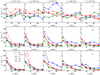 |
Fig. 6. Velocity dispersion profiles measured in pixels of 30 × 30 kpc (Eq. 10) taken along the z-axis (first row) and the y-axis (second row) for the map projected perpendicularly to the jet axis (as indicated by the black dashed lines A and B in Fig. 4) and along the x-direction (third row) for the map projected parallel to the jet axis (as indicated by the black dashed line C in Fig. 5) for runs K1 (blue solid), K05 (green solid), K05np (green dashed), K01 (red solid), and K01np (red dashed) taken at various epochs t = 2.16, 2.86, 3.29, 4.02, and 5.25 Gyr (from left to right). |
The turbulent region expands with time roughly with velocity ≈σx ∼ 100 km/s, which we confound with the characteristic turbulent velocity, rather than the sound speed, about an order of magnitude larger. The other runs have, on average, a lower velocity dispersion (see also Fig. 7), and the region in which the turbulence diffuses is correspondingly smaller.
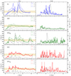 |
Fig. 7. Velocity dispersion of the hot gas (left) and the cold gas phase (right) computed in a region of size 60 × 60 kpc2 with an integration LOS of 150 kpc, projected along the x- (solid), y- (dotted), and z- (dashed) axis, for runs K1, K05, K05np, K01, and K01np (from top to bottom). The gray lines show the evolution of the feedback power at the corresponding times. |
Finally, the third and the fifth panels of Figs. 4 and 5 show the emission weighted projected velocity and velocity dispersion, as seen with a spatial resolution of 30 × 30 kpc, for qualitative comparison with the observations of the Perseus cluster by the Hitomi satellite (Hitomi Collaboration 2016; Simionescu et al. 2019) and future observations with XRISM. For every pixel the projected velocity in that pixel, vpix, is computed using the formula
 (9)
(9)
where the first sum is over the numerical cells in the y − z plane (the plane of the sky) within the pixel area. The second sum is over the cells along the x direction (that is, it performs the integration along the LOS). Likewise, the velocity dispersion σpix in each pixel is computed as
 (10)
(10)
where vpix is from Eq. (9). The sum along the LOS extends out to 300 kpc, to include the contribution of the foreground and background ICM. It should be noticed that, although most of the information related to this X-ray weighted quantity comes from the dense cluster core, which is fully sampled by our procedure, we are neglecting a relatively small contribution from the outer layers in the cluster, due to computing limitations.
It is clear that strong AGN outbursts like the one at t ∼ 3 Gyr for model K1 are easily detectable even at relatively coarse spatial resolution. Both the velocity and the velocity dispersion achieve extreme values ≳250 km/s, just like in the true maps displayed in the second and fourth rows of Figs. 4 and 5. The dilution induced by the decreased resolution do not erase this signature of violent feedback events.
Furthermore, the kinematic maps provide important information about the geometry of the outflows. When the jet axis is almost perpendicular to the LOS, both the velocity and dispersion display a bimodal distribution on the maps, with two highly perturbed regions symmetrically placed with respect to the cluster center (see Fig. 4). On the contrary, when the outflows are aligned with the LOS, only one central peak of velocity and dispersion is present (Fig. 5). During periods of weaker AGN activity, the maps are more homogeneous with average values for the velocity and dispersion reduced by a factor of ≈2 with respect to the activity peak period. To study the geometrical differences due to the LOS just discussed and to compare the velocity dispersion obtained in the other runs, we plot the velocity dispersion profiles taken along two perpendicular directions for the edge-on projection since the distribution appears axi-symmetric, and one for the face-on projection which is symmetric. The first two rows of Fig. 6 show the velocity dispersion profiles of all the runs obtained from the grained maps projected perpendicularly to the jet axis along the z and y direction respectively (as indicated by the dashed black lines A e B of Fig. 4). The third row of Fig. 6 shows the profiles obtained from the grained maps projected parallel to the jet axis along the x direction (as indicated by the dashed black line C of Fig. 5). The velocity dispersion profiles are very different, depending on the considered regions as well as on the feedback modality. In particular, when the jets are observed face-on (third row of Fig. 6) there is a large drop in the σ profile, especially when the AGN activity is strong. The same behavior, with a smaller jump, occurs when we observe the jets edge-on and move perpendicularly to the jet axis (second row of Fig. 6). Conversely, when we see the jets edge-on but we move close to the jet axis, the velocity dispersion profiles show oscillating behaviors when the AGN is active and increasing or decreasing profiles, depending on the run, when the AGN is quiet (late epochs). The shape of each profile is very dependent on the run (i.e., the feedback modality and the presence of precession). We conclude that, while single pointed measurements of the gas velocity dispersion in specific regions of the cluster are generally too affected by time variations to constrain feedback parameters, the full reconstruction of the profile of gas velocity dispersion across a few hundreds of kiloparsecs has the potential to discriminate between different AGN feedback modes.
4.1.2. Evolution of velocity dispersion
The next step is the analysis of the time evolution of the central hot gas velocity dispersion. This is a key quantity to characterize the turbulence or bulk motion of the ICM.
Since we are focusing on only the value of the central region of the cluster, we decide to consider a larger volume, compared to the pixel considered before, of size 60 × 60 kpc2 in the projected plane, with an integration over a LOS of 150 kpc. The first column of Fig. 7 shows the three projections of the velocity dispersion σx, σy and σz, of the hot phase versus time for the models K1, K05, K05np, K01 and K01np (from top to bottom). The velocity dispersion is computed similarly to Eq. (8).
The first thing to note is the strong time correlation between the AGN activity (light gray line) and the velocity dispersion behavior, with the latter showing an increase right after the first powerful AGN burst, and following the later peaks of the AGN feedback during the whole evolution. The correlation is more evident in the runs with a more intermittent AGN activity and is of course expected considering that AGN feedback is here the most relevant driver of gas motions.
The velocity dispersion is strongly anisotropic in the z direction for run K1 and it is also anisotropic for models K05 and K05np, while is almost isotropic in the runs with a major thermal feedback mode, K01 and K01np. Considering the velocity dispersion projected along the LOS perpendicular to the jet axis, which is less directly affected by the initial jet velocity, run K1 shows velocity dispersion values around 200 km/s for most of the time, while during the strong outbursts, it reaches values around 450 km/s. Contrary to K1, run K05 exhibits an almost constant velocity dispersion, with value ∼150 km/s, with little difference among the various projections2. The run K01 and K01np show σ values around 200 km/s, with peaks reaching 300 km/s after strong AGN activities.
It is important to compare the velocity dispersion measure above with the actual measurement of the gas velocity dispersion obtained for the central region of the Perseus cluster by the Hitomi satellite (Hitomi Collaboration 2016; Simionescu et al. 2019), which represents the best constraint on the kinematics of the hot ICM at the center of the cluster to-date. Hitomi measured a relatively quiescent atmosphere, characterized by a gas velocity dispersion of 164 ± 15 km/s in a region of 60 × 60 kpc2 around the core of Perseus. The horizontal golden band in the figure marks the range of values σ = 164 ± 50 km/s. The Table 1 reports the total span of time in which the velocity dispersion stays in these values for all the runs, during the first episode of feedback ≃0.8 Gyr and 6 Gyr. Each different AGN modality gives a different probability of having core motions matching a range of velocity dispersion around the specific value measured by Hitomi in Perseus. The velocity dispersion in run K05 remains in the observed range of values for almost the entire evolution, followed by the thermal runs, K05 and K05np. For the 40% of their evolution (and strongly correlating with strong AGN bursts) run K05np and, even more, run K1 show an excess of gas velocity dispersion well beyond the Hitomi constraint.
Percentage of time during which the velocity dispersion computed in the central region of size 60 kpc stays on the values 164 ± 50 km/s, during 5.2 Gyr, from the first feedback event.
Combined with the results of the previous section, this suggests that, while measurements taken in specific portions of the clusters and at specific times can hardly discriminate among different AGN feedback scenarios, the combination of spatially distributed measurements of gas velocity dispersion, and possibly the complementary measurement of cold gas velocity statistics (see next section) better constrain the actual modality of deposition of feedback energy from AGN.
4.2. Cold phase
Next, we analyze in detail the properties of the cold gas, defined as a gas phase with T < 5 × 10⁴ K. In our simulations, cold gas forms by radiative cooling the hot ICM, with an efficiency that critically depends on the interplay between feedback and precession (or lack thereof). Particularly interesting is the gas which cools off-center, usually at a distance of a few 10s kpc. Such spatially distributed cooling, resulting by sustained, localized compression of the ICM and/or lifting of low entropy gas originally located near the BCG, is thought to play a key role in the feedback process (e.g., Gaspari et al. 2013, 2020; Voit et al. 2017). The physical conditions that lead to off-center cooling have been investigated by many authors (Brighenti & Mathews 2002; Gaspari et al. 2011a,b, 2012; McCourt et al. 2012; Sharma 2013; Li & Bryan 2014a,b; Valentini & Brighenti 2015; Bourne & Sijacki 2017; Beckmann et al. 2019; Qiu et al. 2020; Fournier et al. 2024) who tried to identify the main physical source of the (non-linear) perturbations needed to start the cooling process. Either bulk motion, powered by AGN outflows or cavity buoyancy, turbulence or lifting – more likely a combination of these – can do the trick (see references above). All these processes are effective if and when the susceptibility of the ICM to cool down is high. This property can be quantified through the cooling time tcool, the cooling-to-dynamical time ratio, tcool/tdyn, the entropy parameter T/n2/3, and so on.
The study of the cold gas kinematics is crucial. First, it constrains the origin of cold gas (e.g., Gaspari et al. 2018) and the nature of AGN feedback. Second, cold (ionized and molecular) gas can be observed in great detail with current instruments (Li et al. 2020; Hu et al. 2022; Ganguly et al. 2023; Gingras et al. 2024), and this wealth of data represents a crucial test bed for simulations (see Wang et al. 2021).
In most of our models, the combination of the parameters of the (central) ICM and the perturbations induced by the feedback generates cold gas in an intermittent fashion. We generally find two main types of structures: a population of blob-like cold clumps, often arranged in radial filaments (Fig. A.2), and a central cold rotating disk around the SMBH. In the following, we study several kinematic quantities, like velocity dispersion and the first-order velocity structure function, to characterize the motion of cold gas and its relation with the feedback models.
4.2.1. Cold disk
In a few runs (late epochs of K1 and most of the time of K05) a long-lived rotating cold gas disk, with masses around 1010 M⊙, forms in the very central region of the cluster. Unlike for the case of the cold clumps (see later), we think that the fate of long-lived rotating disks in our simulations is entirely (or mostly) due to the lack of physical ingredients as well as to specific way in which AGN feedback is implemented here, and therefore our predictive power in this region is extremely small. In such high density regions, the physical processes that are expected to govern the long term evolution of the cold gas, like star formation and its consequent feedback are missing in our simulations. There is no radiative feedback from the AGN that is expected to be impactful especially very close to the SMBH. Moreover, all the cold gas chemistry below the set temperature floor of 104 K is missing. Using the same setup, but including star formation, Li et al. (2015) showed that the presence of massive rotating structures is inhibited by the onset of star formation.
Another factor that makes it hard to assess the realism of the forming cold gas is how feedback is numerically implemented here: the jets start in two disks at a certain height from the center and this configuration tends to leave the gas in the center unperturbed, promoting the formation of angular momentum along the vertical axis. Moreover, the formation of angular momentum along a coordinate axis, starting from gas completely at rest, is often found in fixed grid simulations. Conversely, transient events of rotating cold gas that do not end in massive disks should be more realistic.
4.2.2. Cold clumps
Frequently observed structures in our runs are small cold clumps, as also found in Li & Bryan (2014a) and papers quoted above. These clumps are under-resolved in our simulations, with a typical size of 2−10 cells (i.e., 0.5 − 2.5 kpc), often with quasi-spherical shape. This implies that the physical evolution of cold gas cannot be accurately followed. The clumps can form filament-like structures (see models K1 and K05np in Fig. A.2) or they can physically merge, especially in the central region, forming larger blobs. Previous works (e.g., Wang et al. 2021; Ehlert et al. 2023; Das & Gronke 2024; Fournier et al. 2024) have suggested that in the presence of a significant ICM magnetic field, the cold gas naturally assumes a filamentary shape.
A caveat in the cold clumps formation or cold gas in general due to the numerical implementation has to be discussed. As described in Sect. 2.2, new gas mass is added at the jet launching regions, followed by a proportional decrease of gas temperature in order to keep the thermal pressure constant. Thus, the adopted implementation artificially reduces the cooling time of these cells ( in the case of bremsstrahlung losses). It follows that in the outflowing jet material, the formation of thermal instability is numerically accelerated. This potentially important effect might be present in other implementations of AGN feedback and the quantitative impact on the formation of cold clumps will be studied in a future paper.
Nevertheless, the condensation of the cold gas in clumpy or filamentary structures is seen in almost all simulations presented here and in the recent literature. Several general properties of cold gas nebulae (size, location, basic kinematics) agree with observed cool core clusters (e.g., Gaspari et al. 2018), so despite the aforementioned numerical process, which may be acting as a catalyst, the formation of cold gas is a real physical process. The mechanisms which originate the precipitation process are several, from the entrainment by the jets/cavities of low-entropy gas living in or near the cD galaxy to the generation of non-linear perturbations by (subsonic) turbulence or bulk motion (e.g., Brighenti & Mathews 2002; Revaz et al. 2008; Gaspari et al. 2011b; Li & Bryan 2014a; Brighenti et al. 2015; Valentini & Brighenti 2015; McCourt et al. 2012; Voit et al. 2017; Beckmann et al. 2019). Currently, it is not clear which process dominates in real clusters.
4.2.3. Cold gas formation
In the following, we focus on the cold gas structures formed in the different runs. We focus only on that phase of cold gas that it is not accreted at each specific moment onto the SMBH, which represents the potentially observable cold gas mass at each epoch. In reality, the gas that reaches the very center of the cluster is either accreted onto the SMBH or experiences other processes3, but our study aims to analyze the cold gas around the center and to compare its properties to real observations. Of course, if this gas does not get destroyed by heating processes, it will eventually fall into the accretion region so into the SMBH, unless it gets stalled in the long-lived disk.
Figure A.2 (see Fig. 8 for an example) shows the column density of the cold gas projected in a plane parallel to the jet axis at six different epochs, in a time window of ≈700 Myr (from left to right), of the various runs K1, K05, K05np, K01 and K01np (from top to bottom). This figure has to be analyzed jointly with the solid lines of Fig. 9, which show the amount of the cold gas mass formed (that is not accreted in the SMBH) in each run (right panel: runs with precession, left panel: runs without precession) in the central volume of side 150 kpc. Run K1 (first row of Fig. A.2) is one of the runs that form most cold gas, with a maximum of about 2.5 × 10¹⁰ M⊙. The cold gas structure extends out to 100 kpc and 50 kpc along and perpendicularly to the jet axis, appearing as several wide filamentary structures composed of cold clumps raining toward the cluster center. This run forms a stable cold disk after 4 Gyr, that continues accreting until it has reached, 2 Gyr later, a total mass of 1.3 × 10¹⁰ M⊙. The latter is in turn associated with a decreasing power of the jet: the cold circumnuclear gas tends to accrete onto the rotating disk, rather than feed the SMBH.
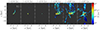 |
Fig. 8. Column density of the cold gas, T < 5 × 10⁴ K, projected on a plane parallel to the jet axis, for various snapshots ranged in less than 1 Gyr (from left to right) of the K1 run. The comparison with the other runs is shown in Fig. A.2. The figure shows the crucial differences in the cold gas formation: run K1 shows the most prominent cold gas structures in a filamentary and clumpy form. Run K05 shows the presence of a long-lived cold gas disk, with very rare formation events of few clumps. While run K05np forms less cold gas compared to runs with precession, it shows a spatially large distribution of cold structures, similar to run K1. Runs K05 and K05np have cold gas structures more localized in the center, with the former, with precession, having more cold gas. |
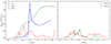 |
Fig. 9. Amount of cold gas mass at each snapshot, and not accreted in the SMBH, i.e., remaining outside the accretion region, computed in volumes of 150 kpc per side (solid line) and of 50 kpc per side (dashed line) for the runs with precession K1, K05, and K01 (right), and without precession K05np and K01np (left). For runs K05, K01, and K01np the lines overlap. |
Run K05 forms a cold disk already soon after the first episode of feedback (≈1 Gyr), and it continues accreting gas during its whole evolution, but it also allows the prolonged accretion of gas onto the SMBH, which overall results into a gentle power history. In this run, there are very rare episodes of cold clumps, and they do not out to a large radius. The disk which accretes continuously throughout the simulation reaches a total mass after 6 Gyr of 2 × 10¹⁰ M⊙ and a size of 10 − 15 kpc. Run K05np shows recurring episodes of clumps formations resulting sometimes in structures of size 100 kpc along the jet axis, but smaller perpendicularly to the jet axis compared to run K1. Overall, it does not form a huge amount of cold gas, having peaks around 6 × 10⁹ M⊙. Runs K01 and K01np produce cold clumps intermittently, in the central region, during the whole evolution, mostly created by a continuous disruption of the disk when it forms. In this case, the cold gas is more localized at the center in a region of size around 40 kpc.
Figure 9 also gives some spatial information about the cold gas distribution: the solid lines measure the cold gas mass of the gas (not accreted on the SMBH) in a central volume of side 150 kpc while the dashed lines show the same quantity computed in a central volume of side 50 kpc. We note that in runs K05, K01, and K01np the lines overlap, meaning that all the cold gas is within the central smaller region, while for run K1 and K05np, there are few epochs in which the 20 − 30% of the cold gas is on larger scales. For this reason, we can compare without ambiguity the kinematic of this phase with the hot phase data obtained in a smaller region.
It is clear now that some runs are more efficient than others in creating cold clumps and accreting them or in breaking the cold disk when it forms. We can relate this trend with the AGN feedback modes and the presence of precession in a qualitative way. Following the ideas of the cold gas formation driven by entrainment of the cold gas by the jets and a formation driven by turbulence at the edge of the jets, we could expect that the kinetic runs, promoting both these processes are the most efficient in creating cold gas. In run K1 the precession helps the turbulence created at the edge of the jets that in turn helps the clump formation. Runs K01 and K01np having a little kinetic part, do not show a large amount of cold gas formation, but still, the precession helps the process since run K01 forms more cold gas than K01np. The absence of precession in the runs with a thermal feedback component discourages the formation of cold gas: these feedback modes heat the ICM mostly in the same regions favoring long-lasting hot bubbles at the same points, preventing the processes of turbulent mixing at their edges and consequent thermal instabilities and cold gas condensation. Run K05np with an important kinetic part produces more cold gas than K01np, but still less than run K01, which has a minor kinetic part but precessing. At variance with this is run K05, in which the cold gas disk that rests untouched for all the simulation accretes all the cold gas that is formed in the run.
4.2.4. Evolution of velocity dispersion
The right panels of Fig. 7 show the velocity dispersion of the cold gas versus time, in the different runs computed in a box of size 150 kpc, computed using Eq. (8), counting only the cells with T < 5 × 10⁴ K. The velocity dispersion of this phase has a very oscillating behavior with maximum values different for each run. A correlation with the AGN activity is hard to find, although in run K1 it seems that σ reaches large values before the AGN activity peaks.
The cold gas in the kinetic run K1 has velocity dispersion values larger with respect to the other runs, as the hot phase does. In particular, it has maximum values around 300 − 500 km/s for a short time. This is due to the cold clumps that form at a certain height close to the vertical axis, and to their motion toward the center, gravitationally driven. After 4 Gyr, the cold gas disk is fully formed, and at this point, the velocity dispersion is very low. In the K05 run, the cold disk is formed after 1 Gyr and so the cold gas kinematic is dominated by that, showing low values of σ. Run K05np shows a cold gas velocity dispersion with the major part of maximum values around 100 km/s and some peaks around 200 − 300 km/s, showing no correlation at all with the AGN activity. Runs K01 and K01np have large values of velocity dispersion reaching 200 − 300 km/s, but the run K01np has some maximum peaks of 500 km/s, in the y and x directions.
Looking at both panels of Figure 7, and comparing the hot and cold phase velocity dispersion, we conclude that the two phases are not significantly coupled. Although the values range around the same numbers sometimes there can be discrepancies of the 30 − 50%.
5. Results: Velocity structure functions
In this section, we analyze the properties of turbulent gas motions by computing the velocity structure functions (VSF) of the hot and cold phases in the various runs. Structure functions of the velocity field are usually employed (together with the complementary view of power spectra) to study other turbulent astrophysical environments (e.g., Kritsuk et al. 2007). A few recent studies investigated turbulence in simulated galaxy clusters using VSF and reported statistics of velocity fluctuations compatible with the Kolmogorov model of turbulence (Kolmogorov 1941) (i.e., VSF ∝ l1/3) for the first-order structure function, or slightly steeper (e.g., Vazza et al. 2009; Li et al. 2020; Wang et al. 2021; Mohapatra et al. 2022; Simonte et al. 2022; Ayromlou et al. 2024). Observations of cold, ionized ICM return detailed information on the VSF, showing that its slope is always steeper than the Kolmogorov prediction, suggesting that the dynamics of cold gas reflects more the feedback driver than the true turbulent cascade (Li et al. 2020; Hu et al. 2022; Ganguly et al. 2023). It is therefore not clear if cold gas is a reliable tracer of hot gas turbulence (Gaspari et al. 2018).
Here we consider the first-order VSF in the i-direction, defined as
 (11)
(11)
The angular brackets ⟨⟩, which theoretically mean the ensemble average, impossible to have in observations, here denote a spatial average. The computation is done in a box of side 150 kpc for both phases. One of the objectives of the analysis is to determine the relation between the observed slope of the VSF, which is intrinsically emission-weighted projected along the LOS, and the real slope of the VSF in 3D, which is strongly linked to the physical properties of the turbulent evolution in the central cluster region.
To infer that, we need the VSF computed using the emission-weighted projected velocities on the plane of the sky, obtained with Eqs. (6) and (7) for the hot and cold phase respectively, in Eq. (11). In that way, we obtain an emission-weighted VSF along the LOS, VSFlos. We compute VSFlos along the three coordinate axes x, y, orthogonal to the axis of the jets, and z parallel to that axis. Then we compare the VSFlos with the intrinsic 3D VSF computed using Eq. (11) substituting the i component of the velocities considering for the hot phase only cells with a temperature above 106 K and for the cold gas cells with T < 5 × 10⁴ K, called so on VSF3D.
5.1. Hot phase VSF
As an example, we show in Fig. 10 the VSF for model K1 computed at t = 2.55 Gyr. We fit the slope of the VSF in a scale range l ≈ [10 − 80] kpc. The peak occurring at scale ∼70 kpc is likely due to the finite box effect, rather than the physical scale of the turbulence driver. At scales ≲10 kpc the slope steepens (this is quite a general property of our models), with slope ∼2/3. However, these scales are close to the simulation resolution (0.25 kpc) and it is unclear how much they reflect a real physical effect.
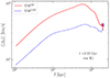 |
Fig. 10. Example of a VSF3D (solid red) and a VSFlos (dashed blue) computed for a snapshot of run K1. |
Figure A.3 (see Fig. 11 for an example) shows the VSF3D (red circles) and VSFlos (blue diamonds) slopes of the x, y and z direction (columns from left to right), of the various runs K1, K05, K05np, K01 and K01np, (rows from top to bottom), computed on a scale range l ≈ [10 − 80 kpc]. The green dotted line shows the jet power of each run and the black dashed line is the Kolmogorov turbulence slope 1/3. We find no obvious general correlation or trend between the VSF3D and VSFlos slopes. Although for most models and most of the time, the two slopes are very close, and some variation happens in phase, it seems not possible to find a general relation between the two VSFs. In the kinetic K1 model there is a tendency for the VSF3D slope to be steeper than the VSFlos one by 20 − 30%. Some runs (K1, K01 and K01np) show a tendency to have the peaks of the two VSFs in phase, but in several cases (first 3 Gyr run K1) the peaks in the VSF3D slopes (i.e., the steepening of the slopes) disappear in the projection, while in other cases (the final part of K1 along the z axis and the x and y VSF of runs K01 and K01np), some steepening of the slopes are enhanced in the projections. A generally expected result is that, since the ICM dynamics is not steady throughout the simulation, the slopes in all models vary with time showing an oscillating behavior. Looking carefully, we note that the VSF3D slope gets steeper after an AGN outburst. We can explain these phenomena considering that the AGN bursts, especially the powerful ones, put in motion gas in larger regions creating bigger vortices and thus increasing the VSF amplitude at bigger scales. During periods of low activities, the VSF slopes become flatter, and trace more closely the turbulence cascade. If we consider that an eddy life τ, is on the order of its turnover time τ ≈ v/l, being v and l its velocity and size, an eddy of 80 kpc moving at 200 km/s, lives less than 500 Myr. In general, the VSF slopes oscillate around the Kolmogorov slope, but most of the time are flatter than it. This contrasts with observations of VSF for the cold phase (see references above).
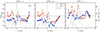 |
Fig. 11. Slopes of the hot gas 3D velocity structure function, VSF3D (red circles), and the projected function, VSFlos (blue diamonds), of the x, y, and z components of velocity and corresponding projection direction (from left to right) fitted in the range 10 − 80 kpc, of run K1. The comparison with the other runs is shown in Fig. A.3. The green dotted lines show the AGN power, while the dashed black line is the Kolmogorov slope. |
5.2. Cold phase VSF
For the cold phase, we compute the VSF3D and the VSFlos based on the projected velocity obtained with Eq. (7). With respect to the hot phase, here we have fewer statistics due to the fact that the cold phase is not volume filling, but clumpy and located in small substructures. For this reason is not possible to have for all the snapshots a VSF for which is possible to measure a slope. Thus, we follow Wang et al. (2021) and average the VSF in time, in order to have enough data to infer some statistical properties. Figure A.4 (see Fig. 12 for an example) shows the VSF3D average during all the time in which the cold gas is present, overplotted on each specific VSF.
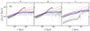 |
Fig. 12. Cold gas phase VSFlos of the x, y, and z components of velocity and corresponding projection direction (from left to right), taken at all the snapshots (gray lines) of run K1. The comparison with the other runs is shown in Fig. A.4. The blue lines show the time average of all the snapshots. The dashed and dotted red lines indicate a slope of 1/3 and 1/2, respectively. |
Again, we find that the cold gas VSF is not steady, but that it reflects the intermittent nature of the AGN feedback. Both the slope and the amplitude vary in time. From the ensemble of gray curves (i.e., of the single VSF3Ds) is evident that after a certain spatial scale the VSFs become too noisy and measuring a slope is impossible. However, we can note that when the VSFs are regular, within a spatial scale varying in time and hardly exceed several kpc, the slopes are steeper than Kolmogorov (as in Li et al. 2020; Wang et al. 2021).
We can also find the moments in which the rotation, that occurs especially around the jet axis, is the dominant kinematic characteristic. Since in run K05 the cold disk is present for most of the time, the resulting VSFs show this physical behavior. Along the x and y directions, the VSF are very steep with slope ≲1 and on the z direction the VSF is flat. This happens in the final Gyr of run K1 and can be spotted for short periods in the other runs.
Concerning the largest scales the time average of the VSF seems to suggest a flattening of the slope. The explanation for the single VSF can be found considering that the cold gas is clumpy and spatially concentrated. Especially the external parts are composed of a small number of clumps, thus the big scales are poorly sampled, given the small number of pairs, resulting in a noisy VSF. Moreover, as we found for the hot gas, the effect of the finite box in which the VSF is computed can give a flattening of the VSF at scales close to the half of the box. In the case of cold gas, the effect of the finite box is natural since the gas is naturally confined in small regions.
On the other hand considering the noise of all the VSFs combined and the fact that they come for different kinematic behavior of the gas, absolutely not steady, we do not trust the sum of all the pairs as reflecting the intrinsic VSF characteristics. Thus the average procedure, even though gives a regular VSF, is not trustworthy as a tracer of the turbulent motion in the cold phase.
6. Discussion and conclusions
In this work we described how we produced new hydrodynamic simulations of AGN feedback in a Perseus-like cluster of galaxies to study the impact of different prescriptions for feedback on the kinematics of the ICM. We investigated models where the BH injects energy with various combinations of kinetic and thermal components. Moreover, we explored the effect of the AGN jet precession on the ICM properties.
A first important finding is that the kinematics of the ICM is strongly correlated with the AGN activity, which is in turn regulated by the feedback mode, and its efficiency in creating cold gas. The accretion of cold gas controls the feedback power, setting the history of the AGN power, which can result in a bursty, intermittent, or gentle regime. In this context, the presence of precession changes the behavior of the AGN, especially for the models in which the feedback energy is mainly deposited as kinetic energy.
The time evolution of the velocity dispersion of the hot and cold gas phases, σhot and σcold (Fig. 7), shows that for the kinetic mode runs it exhibits strong variations, roughly in pace with the AGN activity. However, the peaks of σcold often precede the bursts in the AGN activity, by ≈108 yr, which corresponds to a few dynamical times at the location of the cold gas. Large values for σcold are the signature of the infall of cold clouds toward the central BH, where they are eventually accreted. In contrast to σcold, σhot is tightly correlated with the peaks of AGN power, and this happens for all the models presented here, regardless of the kinetic and/or thermal energy fraction. This agrees overall with the general picture of cold gas feeding the SMBH and causing the hot gas stirring (Gaspari et al. 2012).
However, the velocity dispersion analysis shows that, in general, cold and hot gas velocity dispersion do not perfectly trace each other, but that a discrepancy up to a factor of two is common. In addition to the peak separation in time observed in model K1, σcold displays larger time variations than σhot, an effect that we ascribe to the dominant effect of gravity on the cold clumps. Finally, the time averaged value for σcold is generally lower than σhot. The latter result is in contrast with the findings of Valentini & Brighenti (2015), who found σcold > σhot (see their Fig. 11), and Gaspari et al. (2018), who found instead σcold ∼ σhot, albeit with a dispersion of 30 − 40% (their Fig. 1). Clearly, further investigation must be carried out to clarify the relation between the motion of the various thermal phases of the ICM.
A robust result of our simulations is that the central hot gas velocity dispersion (Fig. 7) agrees with the value observed at the center of Perseus. For more than half of the evolutionary time we found that σhot lies in the observed range (colored band in Fig. 7, Hitomi Collaboration 2016), and this is true for every model presented here. Evidently, the self-regulated AGN activity alone is able to stir the ICM, irrespective of the detail of the feedback nature and numerical implementation. This is also in agreement with what has been found by Truong et al. (2024), who performed zoom-in simulations of clusters in the TNG-cluster simulation. In relaxed Perseus-like clusters, they found a link between the core gas motion and the central engine and argued that SMBH activity can cause high turbulence levels in their core, up to a potentially detectable level. In particular, they showed that with a total cumulative kinetic energy released in the ICM from 1062 up to a few 1062 erg, the resulting velocity dispersion is of 150 − 200 km/s. Ayromlou et al. (2024), using the same simulation suite, also found that the VSF amplitude, which is directly connected to the velocity dispersion, at the core of the cluster is proportional to the AGN activity.
Further information is gained through the analysis of σhot maps (see Fig. 6). The radial profiles along several directions show that different feedback models lead to different geometrical distributions of the velocity dispersion in the cluster core. The magnitude of the velocity dispersion radial drop depends on both the feedback mode and the direction with respect to the LOS. In particular, our calculations show that σhot is about constant along the outflow direction if the jet is seen almost edge-on. This result can be used to verify the presence of large-scale non-relativistic hot gas outflows as a major AGN heating mechanism. Forthcoming data by XRISM telescope will allow spatial analysis of this kind in the brightest cluster cores and will offer observational tests to discriminate among feedback modes, as well as to identify the presence of jet precession.
A more quantitative analysis of the dynamics and turbulence of the multiphase ICM uses the (first-order) velocity structure functions. Our runs show that for the hot gas the slopes of the projected and the intrinsic VSF are similar, but most of the time the VSF3D is slightly steeper than the projected value. In a few cases, however, the opposite happens (Fig. A.3).
This is in contrast with what is expected theoretically, as derived by Xu (2020), who predicted always a steeper slope, due to projection. On the other hand Mohapatra et al. (2022), with a different implementation of turbulence recovered both the effects. We think in our case that the lack of stationary turbulence, and the extreme variability of the driving scale and the driving power, combined with the episodic strong outflows and anisotropy of the turbulent cascade, makes our turbulence system very far from homogeneous and isotropic. This implies that the VSFs are often not single-slope and it is impossible to derive a clear relation between 3D and projected VSF slopes.
This is more evident in the runs with dominant kinetic feedback that injects turbulence into the ICM anisotropically; the VSF3D are always steeper than Kolmogorov during strong outbursts. The steepening of the VSF can be due to AGN-driven coherent outflows and an excess of turbulent eddies at larger scales, combined with a scarcity of small-scale turbulent eddies. Especially for the kinetic run, K1, the steepening in the intrinsic VSF during the strong outburst can be due to the fact that the AGN, in those epochs, is injecting turbulence on large scales, breaking the ideal Kolmogorov cascade model (if present at all). Thus, after the AGN burst, there is a relative excess of large-scale eddies, which have not had time yet to be processed by the Kolmogorov cascade. Therefore, during these moments the dominant projection effect is the cancellation of the large-scale fluctuations due to the apparent smaller distances, leading to a flattening of the VSF.
When the AGN is in a low activity state, the injected turbulence can evolve through the full cascade. When this happens, the discrepancy disappears and the projected VSFs become steeper than the 3D functions, as theoretically predicted. In the end, we found that there is no obvious quantitative connection between the intrinsic and the projected VSF slopes. In principle, although outside of the goal of this paper, further projects can be made by means of controlled experiments in which the AGN feedback power is kept exactly constant among models so that all VSFs are computed for the same overall amount of energy input.
Moreover, we found that most of the time the VSF slope is close to the theoretical Kolmogorov value (1/3), with a tendency to be slightly steeper than Kolmogorov when the VSF is computed in the direction parallel to the AGN jet axis and slightly flatter when computed in the direction perpendicular to the jet axis.
The study of the cold gas VSF is of particular importance, given the wealth of data available via integral field unit spectrographs, both in the optical and submillimeter bands. This is a difficult task for simulations because the internal structure of the cold gas is likely not fully resolved. Our results (Fig. A.4) suggest that performing a time average in all our runs does not yield a slope that corresponds to the true VSF measure at a specific time, which can have a broad range of stochastic behaviors. The single cold gas VSF slopes have a quasi-Kolmogorov slope (∼1/3) in the scale range 1 − 5 kpc and flattening for larger separations, a likely consequence of the finite size of the cold gas system (typical size ≈10 kpc). The observed VSFs for ionized and molecular gas in BCGs show a steeper than Kolmogorov slope (Li et al. 2020; Ganguly et al. 2023), but observations are also affected by projection and smoothing effects, which are not easily quantifiable (see Chen et al. 2023). They also found a flattening of the VSF on larger scales of a pair separation ranging from 1 kpc to 10 kpc, arguing that this is due to the turbulent driving scale. However, the similar physical size of the warm gas nebula might result in a similar flattening. Further theoretical work is needed to securely interpret the VSF computed at separations close to the size of the region considered.
To conclude, we summarize our main results, which are as follows:
-
In self-regulated AGN cycles, different feedback modes and the presence of precession lead to a different efficiency in cold gas formation, which in turn drastically changes the power history of the AGN. As a consequence, the gas velocity dispersion and the VSFs of the hot and the cold gas phases are also different in all cases, suggesting potential pathways to discriminate between different AGN feedback modes.
-
The AGN feedback with different modalities and characteristics is able to produce the hot gas velocity dispersion measured at the center of the Perseus cluster. The powerful test that may constrain which feedback mode is at play is the measurement of velocity dispersion profiles across the central region.
-
Our explored variations of implementations of AGN feedback show that the cold and hot phases are not tightly correlated, with typical discrepancies of 20 − 30% in values of the velocity dispersion of the two phases. The observed time lag between the turbulent statistics of both phases suggests that the cold gas kinematics is more associated with an inflow of the gas while the hot gas kinematics is associated with the outflow from the AGN.
-
The VSF slopes of the hot gas are sensitive to the AGN activity as they get steeper during strong AGN outbursts, especially for those computed along the direction parallel to the jet axis.
-
The VSF slopes, excluding the epoch in which the AGN outbursts make them steep, are close to the Kolmogorov values; they show a tendency to be slightly flatter when computed perpendicularly to the jet axis and slightly steeper when computed parallel to the jet axis.
-
We find no general way to predict the relation between the intrinsic VSF and the projected function, even though some runs show similar behaviors to both and the oscillations in the slopes experienced are in phase.
-
The cold gas VSFs have slopes around ∼1/2 (i.e. steeper than the Kolmogorov value) at small separations l < 5 kpc and become flatter at larger scales, likely because of the finite size of the emitting region.
-
The time average of the VSF is not a good procedure due to the non-steady state of the motion of the phases.
In the future, we plan to test other combinations of feedback modalities and precession properties in order to improve the AGN feedback implementation and to add missing physics at colder gas phases. At the same time, multi-wavelength observations are required for a deeper understanding of these complex processes.
Data availability
Movies associated to Fig. 1 are available at https://www.aanda.org
Sloshing, generated by merging events, can strongly affect the ICM dynamics in the central regions of cool core clusters, but we ignore this process here.
In these computations, the central velocity dispersion is lower than the central one measured in maps and profiles, due to the larger region considered here.
Actually as explained in Sect. 2, all the cold gas reaching the center region of radius 500 pc is removed, but the part that goes in AGN power is only 1% of this mass, this is an attempt of taking in consideration all the difficulties of the gas in reaching effectively the SMBH, as heating processes, the accretion disk and so on.
Acknowledgments
F.V. has been supported by Fondazione Cariplo and Fondazione CDP, through grant n° Rif: 2022-2088 CUP J33C22004310003 for “BREAKTHRU” project.
References
- Ayromlou, M., Nelson, D., Pillepich, A., et al. 2024, A&A, 690, A20 [NASA ADS] [CrossRef] [EDP Sciences] [Google Scholar]
- Babyk, I. V., McNamara, B. R., Tamhane, P. D., et al. 2019, ApJ, 887, 149 [NASA ADS] [CrossRef] [Google Scholar]
- Beckmann, R. S., Dubois, Y., Guillard, P., et al. 2019, A&A, 631, A60 [EDP Sciences] [Google Scholar]
- Bourne, M. A., & Sijacki, D. 2017, MNRAS, 472, 4707 [NASA ADS] [CrossRef] [Google Scholar]
- Bourne, M. A., & Sijacki, D. 2021, MNRAS, 506, 488 [NASA ADS] [CrossRef] [Google Scholar]
- Bourne, M. A., & Yang, H.-Y. K. 2023, Galaxies, 11, 73 [NASA ADS] [CrossRef] [Google Scholar]
- Bourne, M. A., Sijacki, D., & Puchwein, E. 2019, MNRAS, 490, 343 [NASA ADS] [CrossRef] [Google Scholar]
- Brighenti, F., & Mathews, W. G. 2002, ApJ, 573, 542 [Google Scholar]
- Brighenti, F., & Mathews, W. G. 2003, ApJ, 587, 580 [Google Scholar]
- Brighenti, F., & Mathews, W. G. 2006, ApJ, 643, 120 [NASA ADS] [Google Scholar]
- Brighenti, F., Mathews, W. G., & Temi, P. 2015, ApJ, 802, 118 [NASA ADS] [CrossRef] [Google Scholar]
- Bryan, G. L., Norman, M. L., O’Shea, B. W., et al. 2014, ApJS, 211, 19 [Google Scholar]
- Cattaneo, A., & Teyssier, R. 2007, MNRAS, 376, 1547 [NASA ADS] [CrossRef] [Google Scholar]
- Cavagnolo, K. W., Donahue, M., Voit, G. M., & Sun, M. 2009, ApJS, 182, 12 [Google Scholar]
- Chen, M. C., Chen, H.-W., Rauch, M., et al. 2023, MNRAS, 518, 2354 [Google Scholar]
- Churazov, E., Forman, W., Jones, C., Sunyaev, R., & Böhringer, H. 2004, MNRAS, 347, 29 [NASA ADS] [CrossRef] [Google Scholar]
- Cielo, S., Antonuccio-Delogu, V., Silk, J., & Romeo, A. D. 2017, MNRAS, 467, 4526 [NASA ADS] [CrossRef] [Google Scholar]
- Conselice, C. J., Gallagher, J. S., & Wyse, R. F. G. 2001, AJ, 122, 2281 [NASA ADS] [CrossRef] [Google Scholar]
- Das, H. K., & Gronke, M. 2024, MNRAS, 527, 991 [Google Scholar]
- Dubois, Y., Devriendt, J., Slyz, A., & Teyssier, R. 2010, MNRAS, 409, 985 [Google Scholar]
- Dubois, Y., Devriendt, J., Teyssier, R., & Slyz, A. 2011, MNRAS, 417, 1853 [Google Scholar]
- Eckert, D., Ghirardini, V., Ettori, S., et al. 2019, A&A, 621, A40 [NASA ADS] [CrossRef] [EDP Sciences] [Google Scholar]
- Ehlert, K., Weinberger, R., Pfrommer, C., Pakmor, R., & Springel, V. 2023, MNRAS, 518, 4622 [Google Scholar]
- Fabian, A. C. 1994, ARA&A, 32, 277 [Google Scholar]
- Fabian, A. C. 2012, ARA&A, 50, 455 [Google Scholar]
- Fournier, M., Grete, P., Brüggen, M., Glines, F. W., & O’Shea, B. W. 2024, A&A, 691, A239 [NASA ADS] [CrossRef] [EDP Sciences] [Google Scholar]
- Ganguly, S., Li, Y., Olivares, V., et al. 2023, Front. Astron. Space Sci., 10, 1138613 [NASA ADS] [CrossRef] [Google Scholar]
- Gaspari, M., & Churazov, E. 2013, A&A, 559, A78 [NASA ADS] [CrossRef] [EDP Sciences] [Google Scholar]
- Gaspari, M., Brighenti, F., D’Ercole, A., & Melioli, C. 2011a, MNRAS, 415, 1549 [NASA ADS] [CrossRef] [Google Scholar]
- Gaspari, M., Melioli, C., Brighenti, F., & D’Ercole, A. 2011b, MNRAS, 411, 349 [Google Scholar]
- Gaspari, M., Ruszkowski, M., & Sharma, P. 2012, ApJ, 746, 94 [Google Scholar]
- Gaspari, M., Brighenti, F., & Ruszkowski, M. 2013, Astron. Nachr., 334, 394 [NASA ADS] [Google Scholar]
- Gaspari, M., McDonald, M., Hamer, S. L., et al. 2018, ApJ, 854, 167 [Google Scholar]
- Gaspari, M., Tombesi, F., & Cappi, M. 2020, Nat. Astron., 4, 10 [Google Scholar]
- Gatuzz, E., Mohapatra, R., Federrath, C., et al. 2023, MNRAS, 524, 2945 [NASA ADS] [CrossRef] [Google Scholar]
- Gingras, M. J., Coil, A. L., McNamara, B. R., et al. 2024, ArXiv e-prints [arXiv:2404.02212] [Google Scholar]
- Heinz, S., Brüggen, M., & Morsony, B. 2010, ApJ, 708, 462 [Google Scholar]
- Hitomi Collaboration (Aharonian, F., et al.) 2016, Nature, 535, 117 [Google Scholar]
- Hu, Y., Federrath, C., Xu, S., & Mathew, S. S. 2022, MNRAS, 513, 2100 [NASA ADS] [CrossRef] [Google Scholar]
- Hudson, D. S., Mittal, R., Reiprich, T. H., et al. 2010, A&A, 513, A37 [NASA ADS] [CrossRef] [EDP Sciences] [Google Scholar]
- Kolmogorov, A. N. 1941, Akademiia Nauk SSSR Doklady, 32, 16 [NASA ADS] [Google Scholar]
- Kritsuk, A. G., Norman, M. L., Padoan, P., & Wagner, R. 2007, ApJ, 665, 416 [NASA ADS] [CrossRef] [Google Scholar]
- Lau, E. T., Gaspari, M., Nagai, D., & Coppi, P. 2017, ApJ, 849, 54 [NASA ADS] [CrossRef] [Google Scholar]
- Li, Y., & Bryan, G. L. 2012, ApJ, 747, 26 [Google Scholar]
- Li, Y., & Bryan, G. L. 2014a, ApJ, 789, 153 [Google Scholar]
- Li, Y., & Bryan, G. L. 2014b, ApJ, 789, 54 [NASA ADS] [CrossRef] [Google Scholar]
- Li, Y., Bryan, G. L., Ruszkowski, M., et al. 2015, ApJ, 811, 73 [Google Scholar]
- Li, Y., Gendron-Marsolais, M.-L., Zhuravleva, I., et al. 2020, ApJ, 889, L1 [NASA ADS] [CrossRef] [Google Scholar]
- Li, Y., Ganguly, S., Olivares, V., & Su, Y. 2023, American Astronomical Society Meeting Abstracts, 241, 460.18 [Google Scholar]
- Marti-Vidal, I., Marcaide, J. M., Alberdi, A., & Brunthaler, A. 2013, ArXiv e-prints [arXiv:1301.4782] [Google Scholar]
- Mathews, W. G., Faltenbacher, A., & Brighenti, F. 2006, ApJ, 638, 659 [CrossRef] [Google Scholar]
- McCourt, M., Sharma, P., Quataert, E., & Parrish, I. J. 2012, MNRAS, 419, 3319 [NASA ADS] [CrossRef] [Google Scholar]
- McNamara, B. R., Russell, H. R., Nulsen, P. E. J., et al. 2016, ApJ, 830, 79 [Google Scholar]
- Mohapatra, R., Jetti, M., Sharma, P., & Federrath, C. 2022, MNRAS, 510, 2327 [NASA ADS] [CrossRef] [Google Scholar]
- Navarro, J., Frenk, C., & White, S. 1996, ApJ, 462, 563 [NASA ADS] [CrossRef] [Google Scholar]
- Olivares, V., Salome, P., Combes, F., et al. 2019, A&A, 631, A22 [NASA ADS] [CrossRef] [EDP Sciences] [Google Scholar]
- Osterbrock, D. E., & Ferland, G. J. 2006, Astrophysics of Gaseous Nebulae and Active Galactic Nuclei (Sausalito: University Science Books) [Google Scholar]
- Pizzolato, F., & Soker, N. 2005, ApJ, 632, 821 [NASA ADS] [CrossRef] [Google Scholar]
- Pizzolato, F., & Soker, N. 2010, MNRAS, 408, 961 [Google Scholar]
- Qiu, Y., Bogdanović, T., Li, Y., McDonald, M., & McNamara, B. R. 2020, Nat. Astron., 4, 900 [NASA ADS] [CrossRef] [Google Scholar]
- Randall, S. W., Nulsen, P. E. J., Jones, C., et al. 2015, ApJ, 805, 112 [NASA ADS] [CrossRef] [Google Scholar]
- Revaz, Y., Combes, F., & Salomé, P. 2008, A&A, 477, L33 [NASA ADS] [CrossRef] [EDP Sciences] [Google Scholar]
- Sanders, J. S., Fabian, A. C., Smith, R. K., & Peterson, J. R. 2010, MNRAS, 402, L11 [NASA ADS] [CrossRef] [Google Scholar]
- Schure, K. M., Kosenko, D., Kaastra, J. S., Keppens, R., & Vink, J. 2009, A&A, 508, 751 [NASA ADS] [CrossRef] [EDP Sciences] [Google Scholar]
- Sharma, P. 2013, Astron. Soc. India Conf. Ser., 9, 27 [Google Scholar]
- Simionescu, A., Werner, N., Finoguenov, A., Böhringer, H., & Brüggen, M. 2008, A&A, 482, 97 [NASA ADS] [CrossRef] [EDP Sciences] [Google Scholar]
- Simionescu, A., ZuHone, J., Zhuravleva, I., et al. 2019, Space Sci. Rev., 215, 24 [NASA ADS] [CrossRef] [Google Scholar]
- Simonte, M., Vazza, F., Brighenti, F., et al. 2022, A&A, 658, A149 [NASA ADS] [CrossRef] [EDP Sciences] [Google Scholar]
- Soker, N. 2006, New Astron., 12, 38 [Google Scholar]
- Soker, N., & Pizzolato, F. 2005, ApJ, 622, 847 [NASA ADS] [CrossRef] [Google Scholar]
- Truong, N., Pillepich, A., Nelson, D., et al. 2024, A&A, 686, A200 [NASA ADS] [CrossRef] [EDP Sciences] [Google Scholar]
- Ubertosi, F., Giroletti, M., Gitti, M., et al. 2024, A&A, 688, A86 [NASA ADS] [CrossRef] [EDP Sciences] [Google Scholar]
- Valentini, M., & Brighenti, F. 2015, MNRAS, 448, 1979 [NASA ADS] [CrossRef] [Google Scholar]
- Vazza, F., Brunetti, G., Kritsuk, A., et al. 2009, A&A, 504, 33 [NASA ADS] [CrossRef] [EDP Sciences] [Google Scholar]
- Vazza, F., Brunetti, G., Gheller, C., Brunino, R., & Brüggen, M. 2011, A&A, 529, A17 [NASA ADS] [CrossRef] [EDP Sciences] [Google Scholar]
- Vazza, F., Roediger, E., & Brueggen, M. 2012, ArXiv e-prints [arXiv:1202.5882] [Google Scholar]
- Vernaleo, J. C., & Reynolds, C. S. 2006, ApJ, 645, 83 [NASA ADS] [CrossRef] [Google Scholar]
- Voit, G. M., Donahue, M., Bryan, G. L., & McDonald, M. 2015, Nature, 519, 203 [NASA ADS] [CrossRef] [Google Scholar]
- Voit, G. M., Meece, G., Li, Y., et al. 2017, ApJ, 845, 80 [Google Scholar]
- Wang, C., Ruszkowski, M., Pfrommer, C., Oh, S. P., & Yang, H. Y. K. 2021, MNRAS, 504, 898 [NASA ADS] [CrossRef] [Google Scholar]
- Werner, N., Simionescu, A., Million, E. T., et al. 2010, MNRAS, 407, 2063 [NASA ADS] [CrossRef] [Google Scholar]
- Werner, N., Oonk, J. B. R., Sun, M., et al. 2014, MNRAS, 439, 2291 [NASA ADS] [CrossRef] [Google Scholar]
- Xu, S. 2020, MNRAS, 492, 1044 [Google Scholar]
- Yang, H. Y. K., & Reynolds, C. S. 2016, ApJ, 829, 90 [NASA ADS] [CrossRef] [Google Scholar]
- Zhuravleva, I., Churazov, E., Schekochihin, A. A., et al. 2014, Nature, 515, 85 [Google Scholar]
Appendix A: Figures
In this Appendix we put Figs. 3, 8, 11, and 12, which cannot be kept in the text for editorial constraints.
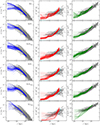 |
Fig. A.1. Gas density (left panels), X-ray emission weighted temperature (center panels), and entropy radial profiles (left panels) obtained at several epochs during the cluster evolution in runs K1, K05, K05np, K01, K01np, and K1np (from top to bottom). The additional gray lines show the distribution of corresponding profiles obtained from the ACCEPT sample by Cavagnolo et al. (2009), for clusters with a central temperature in a range of 3 ≤ T ≤ 5 KeV and a central entropy less than 50KeV/cm2 meant to select cool core cluster with masses close to the Perseus-like cluster simulated. |
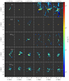 |
Fig. A.2. Column density of the cold gas, T < 5 × 10⁴ K, projected on a plane parallel to the jet axis, for various snapshots ranged in less than 1 Gyr (from left to right), of the five runs K1, K05, K05np, K01, and K01np (from top to bottom). The figure shows the crucial differences in the cold gas formation: run K1 shows the most prominent cold gas structures in a filamentary and clumpy form. Run K05 shows the presence of a long-lived cold gas disk, with very rare formation events of few clumps. While run K05np forms less cold gas compared to runs with precession, it shows a spatially large distribution of cold structures, similar to run K1. Runs K05 and K05np have cold gas structures more localized in the center, with the former, with precession, having more cold gas. |
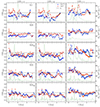 |
Fig. A.3. Slopes of the hot gas 3D velocity structure function, VSF3D (red circles), and projected function, VSFlos (blue diamonds), of the x, y, and z components of velocity and corresponding projection direction (from left to right) fitted in the range 10 − 80 kpc, of run K1, K05, K05np, K01, and K01np (from top to bottom). The green dotted lines show the AGN power, while the dashed black line is the Kolmogorov slope. |
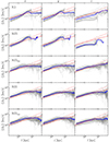 |
Fig. A.4. Cold gas phase VSFlos of the x, y, and z components of velocity and corresponding projection direction (from left to right), taken at all the snapshots (gray lines) of runs K1, K05, K05np, K01, and K01np (from top to bottom). The blue lines show the time average of all the snapshots. The dashed and dotted red lines indicate a slope of 1/3 and 1/2, respectively. |
All Tables
Percentage of time during which the velocity dispersion computed in the central region of size 60 kpc stays on the values 164 ± 50 km/s, during 5.2 Gyr, from the first feedback event.
All Figures
|
Fig. 1. Gas temperature (top) and density (bottom) maps in the x − z plane of the K1, K1np, K05, K05np, K01, and K01np runs (from left to right). The images are not taken at the same absolute time, but rather at the epoch of the maximum AGN feedback power in each run. Movies for the precessing jet simulations can be watched at https://www.youtube.com/watch?v = 7HgSL4xY8lI, https://www.youtube.com/watch?v = 9_SnQm5R8Vs, and online |
| In the text | |
|
Fig. 2. Evolution of the jet feedback power (top) and integrated power (bottom) for the three runs with jet precession (right) K1 (blue dot-dashed), K05 (green dashed), and K01 (red solid), and without precession (left) with the same color and line-coding. |
| In the text | |
|
Fig. 3. Gas density (left), X-ray emission weighted temperature (center), and entropy radial profiles (left) obtained at several epochs during the cluster evolution in run K1. The comparison with the other runs is shown in Fig. A.1. The additional gray lines show the distribution of corresponding profiles obtained from the ACCEPT sample by Cavagnolo et al. (2009) for clusters with a central temperature in a range of 3 ≤ T ≤ 5 KeV and a central entropy less than 50 KeV/cm2 meant to select cool core cluster with masses close to the simulated Perseus-like cluster. |
| In the text | |
|
Fig. 4. Quantities listed in the following at three epochs (from left to right: t = 2.16, 3.29, and 5.25 Gyr) of the kinetic run with precession K1. Top panels: Temperature field in the meridional plane. Second and fourth panels: X-ray emission weighted projected velocity map and corresponding velocity dispersion obtained using Eqs. (6) and (8) along a LOS perpendicular to the jet axis. Third and fifth panels: grained X-ray emission weighted projected velocity and velocity dispersion maps obtained from Eqs. (9) and (10) using a pixel of 30 × 30 kpc along the same LOS perpendicular to the jet axis. |
| In the text | |
|
Fig. 5. Several quantities at three epochs (from left to right: t = 2.16, 3.29, and 5.25 Gyr) of the kinetic run with precession K1. Top panels: Temperature field in a plane perpendicular to the jet axis at 100 kpc from the center. Second and fourth panels: X-ray emission weighted projected velocity map and corresponding velocity dispersion obtained using Eqs. (6) and (8) along the LOS parallel to the jet axis. Third and fifth panels: Grained X-ray emission weighted projected velocity and velocity dispersion maps obtained from Eqs. (9) and (10) using a pixel of 30 × 30 kpc along the LOS parallel to the jet axis. |
| In the text | |
|
Fig. 6. Velocity dispersion profiles measured in pixels of 30 × 30 kpc (Eq. 10) taken along the z-axis (first row) and the y-axis (second row) for the map projected perpendicularly to the jet axis (as indicated by the black dashed lines A and B in Fig. 4) and along the x-direction (third row) for the map projected parallel to the jet axis (as indicated by the black dashed line C in Fig. 5) for runs K1 (blue solid), K05 (green solid), K05np (green dashed), K01 (red solid), and K01np (red dashed) taken at various epochs t = 2.16, 2.86, 3.29, 4.02, and 5.25 Gyr (from left to right). |
| In the text | |
|
Fig. 7. Velocity dispersion of the hot gas (left) and the cold gas phase (right) computed in a region of size 60 × 60 kpc2 with an integration LOS of 150 kpc, projected along the x- (solid), y- (dotted), and z- (dashed) axis, for runs K1, K05, K05np, K01, and K01np (from top to bottom). The gray lines show the evolution of the feedback power at the corresponding times. |
| In the text | |
|
Fig. 8. Column density of the cold gas, T < 5 × 10⁴ K, projected on a plane parallel to the jet axis, for various snapshots ranged in less than 1 Gyr (from left to right) of the K1 run. The comparison with the other runs is shown in Fig. A.2. The figure shows the crucial differences in the cold gas formation: run K1 shows the most prominent cold gas structures in a filamentary and clumpy form. Run K05 shows the presence of a long-lived cold gas disk, with very rare formation events of few clumps. While run K05np forms less cold gas compared to runs with precession, it shows a spatially large distribution of cold structures, similar to run K1. Runs K05 and K05np have cold gas structures more localized in the center, with the former, with precession, having more cold gas. |
| In the text | |
|
Fig. 9. Amount of cold gas mass at each snapshot, and not accreted in the SMBH, i.e., remaining outside the accretion region, computed in volumes of 150 kpc per side (solid line) and of 50 kpc per side (dashed line) for the runs with precession K1, K05, and K01 (right), and without precession K05np and K01np (left). For runs K05, K01, and K01np the lines overlap. |
| In the text | |
|
Fig. 10. Example of a VSF3D (solid red) and a VSFlos (dashed blue) computed for a snapshot of run K1. |
| In the text | |
|
Fig. 11. Slopes of the hot gas 3D velocity structure function, VSF3D (red circles), and the projected function, VSFlos (blue diamonds), of the x, y, and z components of velocity and corresponding projection direction (from left to right) fitted in the range 10 − 80 kpc, of run K1. The comparison with the other runs is shown in Fig. A.3. The green dotted lines show the AGN power, while the dashed black line is the Kolmogorov slope. |
| In the text | |
|
Fig. 12. Cold gas phase VSFlos of the x, y, and z components of velocity and corresponding projection direction (from left to right), taken at all the snapshots (gray lines) of run K1. The comparison with the other runs is shown in Fig. A.4. The blue lines show the time average of all the snapshots. The dashed and dotted red lines indicate a slope of 1/3 and 1/2, respectively. |
| In the text | |
|
Fig. A.1. Gas density (left panels), X-ray emission weighted temperature (center panels), and entropy radial profiles (left panels) obtained at several epochs during the cluster evolution in runs K1, K05, K05np, K01, K01np, and K1np (from top to bottom). The additional gray lines show the distribution of corresponding profiles obtained from the ACCEPT sample by Cavagnolo et al. (2009), for clusters with a central temperature in a range of 3 ≤ T ≤ 5 KeV and a central entropy less than 50KeV/cm2 meant to select cool core cluster with masses close to the Perseus-like cluster simulated. |
| In the text | |
|
Fig. A.2. Column density of the cold gas, T < 5 × 10⁴ K, projected on a plane parallel to the jet axis, for various snapshots ranged in less than 1 Gyr (from left to right), of the five runs K1, K05, K05np, K01, and K01np (from top to bottom). The figure shows the crucial differences in the cold gas formation: run K1 shows the most prominent cold gas structures in a filamentary and clumpy form. Run K05 shows the presence of a long-lived cold gas disk, with very rare formation events of few clumps. While run K05np forms less cold gas compared to runs with precession, it shows a spatially large distribution of cold structures, similar to run K1. Runs K05 and K05np have cold gas structures more localized in the center, with the former, with precession, having more cold gas. |
| In the text | |
|
Fig. A.3. Slopes of the hot gas 3D velocity structure function, VSF3D (red circles), and projected function, VSFlos (blue diamonds), of the x, y, and z components of velocity and corresponding projection direction (from left to right) fitted in the range 10 − 80 kpc, of run K1, K05, K05np, K01, and K01np (from top to bottom). The green dotted lines show the AGN power, while the dashed black line is the Kolmogorov slope. |
| In the text | |
|
Fig. A.4. Cold gas phase VSFlos of the x, y, and z components of velocity and corresponding projection direction (from left to right), taken at all the snapshots (gray lines) of runs K1, K05, K05np, K01, and K01np (from top to bottom). The blue lines show the time average of all the snapshots. The dashed and dotted red lines indicate a slope of 1/3 and 1/2, respectively. |
| In the text | |
Current usage metrics show cumulative count of Article Views (full-text article views including HTML views, PDF and ePub downloads, according to the available data) and Abstracts Views on Vision4Press platform.
Data correspond to usage on the plateform after 2015. The current usage metrics is available 48-96 hours after online publication and is updated daily on week days.
Initial download of the metrics may take a while.