| Issue |
A&A
Volume 697, May 2025
|
|
|---|---|---|
| Article Number | A46 | |
| Number of page(s) | 13 | |
| Section | Extragalactic astronomy | |
| DOI | https://doi.org/10.1051/0004-6361/202452461 | |
| Published online | 05 May 2025 | |
Going deeper into the dark with COSMOS-Web
JWST unveils the total contribution of radio-selected NIR-faint galaxies to the cosmic star formation rate density
1
CEA, IRFU, DAp, AIM, Université Paris-Saclay, Université Paris Cité, Sorbonne Paris Cité, CNRS, 91191 Gif-sur-Yvette, France
2
University of Bologna, Department of Physics and Astronomy (DIFA), Via Gobetti 93/2, I-40129 Bologna, Italy
3
INAF – Osservatorio di Astrofisica e Scienza dello Spazio, via Gobetti 93/3, 40129 Bologna, Italy
4
Technical University of Munich, TUM School of Natural Sciences, Department of Physics, James-Franck-Str. 1, 85748 Garching, Germany
5
Max-Planck-Institut für Astrophysik, Karl-Schwarzschild-Str. 1, 85748 Garching, Germany
6
SISSA, Via Bonomea 265, I-34136 Trieste, Italy
7
INAF/IRA, Istituto di Radioastronomia, Via Piero Gobetti 101, 40129 Bologna, Italy
8
Department of Astronomy, University of Geneva, Chemin Pegasi 51, CH-1290 Versoix, Switzerland
9
Institute for Astronomy, School of Physics & Astronomy, University of Edinburgh, Royal Observatory, Edinburgh EH9 3HJ, UK
10
The University of Texas at Austin, 2515 Speedway Boulevard Stop C1400, Austin, TX 78712, USA
11
Department of Physics and Astronomy, University of Hawaii, Hilo, 200 W Kawili St, Hilo, HI 96720, USA
12
Caltech/IPAC, MS314-6, 1200 E. California Blvd., Pasadena, CA 91125, USA
13
Cosmic Dawn Center at the Niels Bohr Institute, University of Copenhagen and DTU-Space, Technical University of Denmark, Denmark
14
DTU-Space, Technical University of Denmark, Elektrovej 327, DK-2800 Kgs. Lyngby, Denmark
15
Niels Bohr Institute, University of Copenhagen, Jagtvej 128, DK-2200 Copenhagen, Denmark
16
Center for Computational Astrophysics, Flatiron Institute, 162 Fifth Avenue, New York, NY 10010, USA
17
Aix Marseille Univ, CNRS, CNES, LAM, Marseille, France
18
IFPU – Institute for fundamental physics of the Universe, Via Beirut 2, 34014 Trieste, Italy
19
INFN-Sezione di Trieste, via Valerio 2, 34127 Trieste, Italy
20
Inter-University Institute for Data Intensive Astronomy, Department of Astronomy, University of Cape Town, 7701 Rondebosch, Cape Town, South Africa
21
Inter-University Institute for Data Intensive Astronomy, Department of Physics and Astronomy, University of the Western Cape, 7535 Bellville, Cape Town, South Africa
22
Laboratory for Multiwavelength Astrophysics, School of Physics and Astronomy, Rochester Institute of Technology, 84 Lomb Memorial Drive, Rochester, NY 14623, USA
23
Institut d’Astrophysique de Paris, UMR 7095, CNRS, and Sorbonne Université, 98 bis boulevard Arago, F-75014 Paris, France
24
Space Telescope Science Institute, 3700 San Martin Drive, Baltimore, MD 21218, USA
25
Purple Mountain Observatory, Chinese Academy of Sciences, 10 Yuanhua Road, Nanjing 210023, China
26
Jet Propulsion Laboratory, California Institute of Technology, 4800 Oak Grove Drive, Pasadena, CA 91001, USA
27
Department of Physics and Astronomy, UCLA, PAB 430 Portola Plaza, Box 951547 Los Angeles, CA 90095-1547, USA
28
Department of Astronomy and Astrophysics, University of California, Santa Cruz, 1156 High Street, Santa Cruz, CA 95064, USA
⋆ Corresponding author: fabrizio.gentile@cea.fr
Received:
2
October
2024
Accepted:
28
February
2025
We present the first follow-up with JWST of radio-selected near-infrared (NIR)-faint galaxies as part of the COSMOS-Web survey. By selecting galaxies detected at radio frequencies (S3 GHz > 11.5 μJy; i.e., S/N > 5) and with faint counterparts at NIR wavelengths (F150W > 26.1 mag), we collected a sample of 127 likely dusty star-forming galaxies (DSFGs). We estimated their physical properties through SED fitting, computed the first radio luminosity function for these types of sources and their contribution to the total cosmic star formation rate density. Our analysis confirms that these sources represent a population of highly dust-obscured (⟨Av⟩∼3.5 mag) massive (⟨M⋆⟩∼1010.8 M⊙) and star-forming galaxies (⟨SFR⟩∼300 M⊙ yr−1) located at ⟨z⟩∼3.6, representing the high-redshift tail of the full distribution of radio sources. Our results also indicate that these galaxies could dominate the bright end of the radio luminosity function and reach a total contribution to the cosmic star formation rate density equal to that estimated only considering NIR-bright sources at z ∼ 4.5. Finally, our analysis further confirms that the radio selection can be employed to collect statistically significant samples of DSFGs, representing a complementary alternative to the other selections based on JWST colors or detection at FIR/(sub)millimeter wavelengths.
Key words: galaxies: evolution / galaxies: high-redshift / galaxies: ISM / galaxies: starburst / infrared: galaxies / submillimeter: galaxies
© The Authors 2025
 Open Access article, published by EDP Sciences, under the terms of the Creative Commons Attribution License (https://creativecommons.org/licenses/by/4.0), which permits unrestricted use, distribution, and reproduction in any medium, provided the original work is properly cited.
This article is published in open access under the Subscribe to Open model. Subscribe to A&A to support open access publication.
1. Introduction
Understanding how galaxies evolved from the Big Bang to the present time is one of the main open questions of modern astrophysics. The answer is commonly thought to reside in deep galaxy surveys, which collect objects at different cosmic times and potentially unveil their evolutionary links. Most of these surveys are performed at optical and near-IR (NIR) wavelengths. Therefore – at z > 3 – these surveys sample a spectral range more affected by dust extinction (see e.g., Salim & Narayanan 2020, for a review). For this reason, a population of dust-obscured galaxies is constantly missed by these surveys, potentially biasing all the results achieved with them (e.g., Simpson et al. 2014; Franco et al. 2018; Wang et al. 2019; Talia et al. 2021; Enia et al. 2022; Behiri et al. 2023; Barrufet et al. 2023; Gottumukkala et al. 2024; Gentile et al. 2024a; Williams et al. 2024). These dusty star-forming galaxies (DSFGs) lacking a counterpart at optical/NIR wavelengths have assumed several names: HST-dark, H-dropout, NIR-dark, OIR-dark, and NIR-faint galaxies. All of these classifications are commonly based on the lack of a counterpart in the optical/NIR regimes coupled with a bright flux at longer wavelengths, potentially tracing ongoing star formation. These tracers can be in the mid-IR (MIR; see e.g., Wang et al. 2019; Barrufet et al. 2023; Gottumukkala et al. 2024; Williams et al. 2024), (sub)millimeter (e.g., Simpson et al. 2014; Franco et al. 2018; Gruppioni et al. 2020; Smail et al. 2021) or radio (e.g., Chapman et al. 2001; Talia et al. 2021; Enia et al. 2022; Behiri et al. 2023; van der Vlugt et al. 2023; Gentile et al. 2024a). Regardless of the selection, several studies targeting these sources agree that they represent a population of massive (M⋆ > 1010 M⊙) and dust-obscured (Av > 3 mag) galaxies mainly located at z ∼ 2 − 3 and beyond. However, a consensus is still missing about their actual contribution to the cosmic star formation rate density (SFRD; i.e., the average amount of stellar mass formed in the Universe each year and in each cubic Megaparsec; see e.g., the results by Wang et al. 2019; Talia et al. 2021; Enia et al. 2022; Barrufet et al. 2023; Behiri et al. 2023; van der Vlugt et al. 2023; Williams et al. 2024), the overlap between the different populations (e.g., Smail et al. 2002; Talia et al. 2021; McKinney et al. 2025; Williams et al. 2024), and their relationship with the broader population of galaxies (e.g., Cochrane et al. 2024).
The advent of the James Webb Space Telescope (JWST) jas provided the opportunity to study these populations on a common ground. Its unprecedented sensitivity allows one to detect – for the first time – the rest-frame optical radiation from these sources, reducing the uncertainties on their photometric redshifts and stellar masses (see e.g., Barrufet et al. 2023; Gottumukkala et al. 2024), and – more broadly – to fairly compare the different populations (see e.g., Pérez-González et al. 2023; Gillman et al. 2024; Hodge et al. 2025; McKinney et al. 2025).
In this paper, we focus on the radio-selected NIR-faint galaxies (Talia et al. 2021). These sources are defined as radio-detected sources without a counterpart in the optical/NIR regimes at the depths commonly reached by ground-based facilities (25–27 mag; see e.g., Weaver et al. 2022). Given radio is a dust-unbiased tracer of star formation (see e.g., Kennicutt & Evans 2012), these sources are excellent DSFG candidates (see e.g., Chapman et al. 2001; Talia et al. 2021; Enia et al. 2022; Behiri et al. 2023; Gentile et al. 2024a).
Compared with other possible methods to collect DSFGs, the radio selection presents some advantages. Firstly, the higher resolution and sensitivity of radio interferometers than previous generation facilities observing at far-infrared (FIR) or (sub)millimeter wavelengths (with beam sizes larger than 10″; see e.g., Swinyard et al. 2010; Dempsey et al. 2013) such as Herschel or the SCUBA-2 camera equipped on the James Clerk Maxwell Telescope (JCMT; see e.g., the initial studies in this field by Smail et al. 1997; Hughes et al. 1998; Burgarella et al. 2013; Gruppioni et al. 2013; Casey et al. 2014, for a review). These properties allow for the easier association of multi-wavelength counterparts and the discovery of fainter sources. Moreover, the higher mapping speed of radio interferometers with respect to modern facilities such as the Atacama Large Millimetre Array (ALMA) or the NOrtern Extended Millimetre Array (NOEMA) makes it possible to explore larger cosmic volumes and – therefore – obtain larger samples less affected by cosmic variance and poor statistics. Secondly, the radio selection is expected to be more robust to the contamination by red and passive galaxies affecting the MIR selection (see e.g., the fraction of non-dusty sources reported in the MIR-selected samples by Wang et al. 2019; Pérez-González et al. 2023; Barrufet et al. 2025).
The downside of such selection is represented, on the one hand, by the positive k-correction at radio frequencies, limiting our possibilities to select very high-z DSFGs that are more easily detected at (sub)millimeter wavelengths (due to to the negative k-correction in that regime; see e.g., Casey et al. 2021). On the other hand, the radio selection needs to take into account the possible contribution by active galactic nuclei (AGN; which are also able to emit at radio frequencies, see e.g., the review by Tadhunter 2016). To do so, we focus on the sources detected in the COSMOS field, which is one of the most famous extra-galactic fields in modern astronomy (see e.g., Scoville et al. 2007; Koekemoer et al. 2007) and has good photometric coverage from radio to X-rays, allowing us to estimate the AGN contribution to our sample of targets with the help of ancillary data. We also take advantage of the new JWST coverage of the COSMOS field granted by the COSMOS-Web survey (Casey et al. 2023).
The main goals of this work consist of the estimation of the physical properties of these sources, their first radio luminosity function (never estimated before for NIR-dark/faint galaxies), and – consequently – their contribution to the cosmic SFRD. These results will then be employed to compare our targets with other notable populations of optically/NIR-faint galaxies in the current literature.
The paper is structured as follows. In Section 2, we describe the data and the sample selection. In Section 3, we estimate the physical properties of our targets through SED fitting and the possible AGN contribution. In Section 4, we estimate the luminosity function of our sources, and in Section 5, we use this result to compute how much our galaxies contribute to the cosmic SFRD. We discuss our results in Section 6, and – finally – we draw our conclusions in Section 7.
Throughout this paper, we assume a standard flat ΛCDM cosmology with the parameters [h, ΩM, ΩΛ]=[0.7, 0.3, 0.7]. We also assume a Chabrier (2003) initial mass function and the AB photometric system (Oke & Gunn 1983).
2. Data
2.1. JWST photometry
The JWST photometry for our sources comes from the COSMOS-Web survey (GO #1727, PIs Kartaltepe & Casey; Casey et al. 2023), a cycle 1 treasury program consisting of the NIRCam and MIRI imaging of the COSMOS field. The program includes a contiguous NIRCam mosaic covering the central region of the field (∼0.54 deg2) in the four filters: F115W, F150W (the short-wavelength filters; SW hereafter), F277W, and F444W (long-wavelength; LW). In parallel with the NIRCam mosaic, COSMOS-Web also includes a MIRI mosaic covering a total (non-contiguous) area of 0.19 deg2 in the F770W filter. A full description of the COSMOS-Web program can be found in Casey et al. (2023), while the data reduction procedure is described in detail in Franco et al. (in prep.).
In this work, we use the NIRCam and MIRI photometry extracted with SourceXtractor++ (SE++; Bertin et al. 2020; Kümmel et al. 2020). This software performs the detection on a positive-truncated χ2 combination of the four NIRCam filters with the point spread function (PSF) homogenized to F444W. Each source is then modeled with a Sérsic profile (Sérsic 1963). The best-fitting model is then convolved with the PSFs of the five (NIRCam and MIRI; PSF FWHM = 0.04–0.14″ and 0.27″, respectively) scientific maps in order to extract the fluxes and the related uncertainties. The full catalog includes photometry for more than 800 000 sources down to a 5σ limiting magnitude of m = 28.0 in F444W. A full description of the procedure that was followed to build the COSMOS-Web catalogs can be found in Shuntov, Paquereau et al. (in prep.).
2.2. Radio data
The radio data analysed in this paper come from the VLA-COSMOS Large Program (Smolčić et al. 2017), a radio survey performed with the Karl Jansky Very Large Array (VLA) covering the full COSMOS field (∼2 deg2) at a frequency of 3 GHz. The survey reaches a quite uniform rms of σ = 2.3 μJy beam−1 and a spatial resolution of 0.75″. To perform our sample selection, we crossmatch the photometric catalog of COSMOS-Web with the public catalog by Smolčić et al. (2017) with a matching radius of 0.7″ (as in Gentile et al. 2024a). This procedure gives as an output a sample of 3196 galaxies. However, given the better spatial resolution of NIRCam than that achieved with the VLA, 139 radio sources have multiple NIRCam galaxies falling in the matching radius. Given the impossibility to recognize the actual object originating the radio emission, we exclude these sources from the final sample.
2.3. Sample selection
We perform a sample selection resembling those employed by Talia et al. (2021), Behiri et al. (2023), and Gentile et al. (2024a) to collect their sample of “radio-selected NIRdark galaxies” in the COSMOS field but taking advantage of the new JWST photometry coming from the COSMOS-Web survey. We start from the parent sample assembled in Section 2.2 and we select our galaxies through the following criteria:
Clearly – by construction – all the galaxies in the final sample also need to be detected in the detection image employed to assemble the COMSOS-Web catalog.
The first criterion requires that the sources are robustly (S/N > 5) detected at radio frequencies, while the latter requires that they would not be detected in the NIR filter H (λ ∼ 1.6 μm) at the 3σ depth of the COSMOS2020 catalog (2″ aperture; see Weaver et al. 2022). The full sample includes 127 galaxies in the 0.54 deg2 observed in the COSMOS-Web survey (55 with MIRI coverage, ∼32% of the full sample, 44 with a robust detection at S/N > 3).
Compared with the previous criteria employed by Talia et al. (2021), Behiri et al. (2023), and Gentile et al. (2024a), we include in our sample sources with lower values of the S/N at 3 GHz. The previous studies, indeed, employed a S/N > 5.5 cut to reduce the number of possible spurious sources. However, the availability of a strong prior such as the NIRCam imaging allows us to relax this criterion, potentially including in our sample some higher-z sources previously missed due to their faintness at radio frequencies (e.g., the spectroscopically confirmed source at z ∼ 5 reported by Jin et al. 2019, with a reported S/N at 3 GHz of 5.2).
Moreover, those studies required the lack of counterpart in the COSMOS2020 catalog, whose detection was performed on a χ2-image including the four VISTA filters Y, J, H, and Ks and the two optical filters i and z from HSC (Weaver et al. 2022). However, the low resolution of these images did not completely allow a counterpart-matching for some optically bright galaxies blended with nearby sources (see the discussion in Gentile et al. 2024a). With these improved criteria and with the high-resolution of the NIRCam maps, we aim to select a less contaminated sample of “NIRdark” galaxies. Since these sources are now detected at the new depths reached by NIRCam, in the following we will refer to our galaxies as radio-selected NIR-faint (RS-NIR-faint).
2.4. Ancillary data
Our targets are located in the COSMOS field. Therefore, an almost complete photometric coverage is available for them. We include in our analysis the following data:
-
Optical-to-MIR: The SE++ software employed to extract the NIRCam and MIRI photometry can also be applied to other ancillary data, by fitting each source with the parametric model computed on the NIRCam maps (once convolved with the PSF of low-resolution maps). These additional data include optical, NIR, and MIR data. The optical maps are obtained during the Subaru Strategic Program (SSP DR3; Aihara et al. 2019) performed with the HyperSupreme Cam (HSC) mounted on the Subaru telescope and those obtained with the Advanced Camera for Surveys (ACS) equipped on HST (Koekemoer et al. 2007). The NIR data are obtained during the UltraVISTA survey (DR6; McCracken et al. 2012) performed with the VIRCAM instrument of the VISTA telescope. Finally, the MIR data obtained as part of the Cosmic Dawn Survey of the COSMOS field (Euclid Collaboration: Moneti et al. 2022) performed with the Infrared Array Camera (IRAC) equipped on the Spitzer Space Telescope. The footprint of all these surveys overlap with the full COSMOS-Web area. In order to cover wavelength ranges not included in our NIRCam and MIRI photometry, we include in our catalog the data in the eight filters g, r, i, z, y, F814W, Ks and in the first channel of IRAC (λ ∼ 3.8 μm). The depths and additional details on the employed maps can be found in Weaver et al. (2022) and in Shuntov, Paquereau et al. (in prep.).
-
FIR/(sub)mm: We crossmatch our catalog with the most updated version of the super-deblended catalog (Jin et al. 2018, and in prep.), including deblended photometry from the PACS and SPIRE instruments equipped on the Herschel space telescope that observed the COSMOS field during the surveys described in Lutz et al. (2011) and Oliver et al. (2012). From the same catalog, we also retrieve photometry at 870 μm from the deblending of the SCUBA-2 maps obtained during the S2COSMOS survey by Simpson et al. (2019). Since the super-deblended employs the 3 GHz sources of the VLA-COSMOS survey as priors, all our galaxies have an entry in that catalog. More in detail, 72 sources in our sample have at least one detection at S/N > 3 in at least one PACS or SPIRE filter. Similarly, 31 objects are detected at S/N > 3 in the 870 μm maps. All the other objects have upper limits. We also obtain ALMA photometry in the (sub)millimeter range for 38 of our sources (∼30% of the sample) by crossmatching with the most recent catalog (v20220606) from the Automated mining of the public ALMA Archive in the COSMOS field (A3COSMOS; Liu et al. 2019; Adscheid et al. 2024).
-
Radio: Finally, we retrieve data at radio frequencies (3, 1.4, and 1.28 GHz) by crossmatching with the public catalogs from the VLA-COSMOS large program (Smolčić et al. 2017; Schinnerer et al. 2007) and the early data release of the MIGHTEE survey performed with MeerKAT (Jarvis et al. 2016). Given the lower resolution of the MIGHTEE maps (∼8″), we only consider the 1.28 GHz radio fluxes of 84 isolated sources (i.e., without another 3 GHz object within 8″).
3. SED fitting
Our SED fitting is performed with the “Code Investigating GALaxy Emission” (Cigale; Boquien et al. 2019), a software based on the principle of energy balance between the dust attenuation and its thermal emission at longer wavelengths. The input catalog includes all the photometry available for our sources with the only exception of the radio data (employed later to estimate the AGN fraction in our sources; see Section 3.3). Our setup includes the stellar populations by Bruzual & Charlot (2003), combined through a delayed exponentially declining star formation history with an additional recent burst of star formation. The stellar emission is extincted through a Charlot & Fall (2000) attenuation law, while the dust emission is included in our templates through the models by Draine et al. (2014). Finally, the nebular emission is accounted for through a series of models computed with Cloudy (Ferland et al. 2013). The resulting templates are redshifted on a grid spanning the range z ∈ [0, 8] with a step of 0.05. The full list of parameters employed in our SED fitting is included in the Appendix A. The good convergence of the SED-fitting procedure is ensured by the distribution of the reduced χ2, with a median value of ⟨χν2⟩ = 1.1 and 95% of the sample with a χν2 < 5. Some examples of the SED-fitting output are reported in Figure 1.
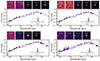 |
Fig. 1. Some examples of the SED fitting performed with Cigale on the galaxies included in the highest redshift bin. The squares indicate the photometric points from JWST, A3COSMOS and the 870 μm from the deblending of the S2COSMOS maps by Simpson et al. (2019). The circular points report the ancillary photometry from HSC, VISTA, Spitzer, and from the super-deblending of the Herschel Maps. The inset shows the Gaussianized p(z) computed with Cigale. The top row shows the cutouts (3 arcsec side) in the NIRCam and MIRI filters of COSMOS-Web. |
3.1. Photometric redshifts
The distribution of the photometric redshifts for our sources is reported in Figure 2 (the other samples showed for reference are described in detail in Section 6.1). The distribution is quite peaked at ⟨z⟩∼3.6, with a 1σ dispersion (given as the symmetrized interval between the 16th and the 84th percentile) of 0.8. The availability of the new NIRCam and MIRI photometry allows us to sample the rest-frame optical/NIR emission of our galaxies, reducing the uncertainty on the photometric redshifts. The median δz/(1 + z) for our galaxies is 0.08, nearly half of what we would obtain by removing the JWST photometry from the SED fitting performed with Cigale (0.15). The spectroscopic coverage of our sample is not sufficient to allow proper testing of our photometric redshift. However, thanks to the collection of spectroscopic redshift in COSMOS (Khostovan et al., in prep.), we found four sources in our sample with a spec-z. These are ID20010161 (zspec = 5.051) from Jin et al. (2019) (see also Gentile et al. 2024b) and AS2COS0002 (zspec = 4.600), AS2COS0011 (zspec = 4.783), and AS2COS0014 (zspec = 2.920) from Chen et al. (2022). These spectroscopic redshifts are well recovered by our SED fitting, with the first three objects having a discrepancy lower than 2σ and only the last one having a spec-z at 5σ from the photo-z. The median value (computed on this small sample) of the |Δz|/(1 + z) is 0.09.
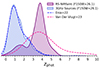 |
Fig. 2. Distribution of the photometric redshifts of our RS-NIR-faint galaxies in COSMOS-Web. Our sources are reported as the purple solid line, while the complementary sample of 3 GHz objects with F150W > 26.1 mag is reported as the blue solid line. For reference, we also show the photo-z computed by Enia et al. (2022) on their sample of radio sources (with optical/NIR counterparts) in the GOODS-N field (blue dashed line) and those estimated by van der Vlugt et al. (2023) for their sample of optically/NIR-faint galaxies in their deeper COSMOS-XS survey (dashed pink line). |
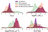 |
Fig. 3. Main properties (photometric redshift, stellar mass, SFR, and dust extinction) of our RS-NIR-faint galaxies. We show – for comparison – the same properties computed by Gottumukkala et al. (2024) and McKinney et al. (2025) for their sample of JWST-selected and SCUBA-selected DSFGs as the green and orange solid lines, respectively. To allow a fair comparison, we only include the sources by Gottumukkala et al. (2024) with F150W > 26.1 mag and exclude the sources flagged as possible AGN. |
3.2. Physical properties
With Cigale, we also estimate the stellar masses and dust attenuation for our galaxies. Since we do not have any constraints on the rest-frame UV SED of our sources, we do not use the SFR computed through SED fitting for our analysis. Instead, we compute the SFR from the radio luminosity – after accounting for the possible AGN contribution – as described in Section 3.31. The results of this procedure are summarized in Table 1 and in Figure 3. These distributions picture the RS-NIR-faint galaxies as a population of highly dust-obscured (⟨Av⟩∼3.5 mag), massive (⟨M⋆⟩∼1010.8 M⊙) and star-forming galaxies (⟨SFR⟩∼300 M⊙ yr−1) located at ⟨z⟩∼3.6. Figure 3 also shows for reference the same properties computed for other notable populations of dusty star-forming galaxies (i.e., those selected with JWST by Gottumukkala et al. 2024 and with SCUBA/ALMA by McKinney et al. 2025). A full comparison between the RS-NIR-faint galaxies and these other samples will be the focus of Section 6.1.
Median properties of our RS-NIR-faint galaxies.
3.3. AGN contribution
Since we are dealing with galaxies selected at radio frequencies, we need to consider that part of that emission could be due to nuclear activity and not to star formation. For doing so, we follow the procedure established by Ceraj et al. (2018) to measure the so-called “AGN fraction” (fAGN), quantifying the AGN contribution to the radio luminosity.
We start by computing the infrared luminosity (LIR) of our sources by integrating the best-fitting SED given in output by Cigale in the range [8,1000] μm. The LIR is then employed to compute the qTIR parameter (quantifying the ratio between infrared and radio emission) for our galaxies as
![$$ \begin{aligned} q_{\rm TIR}= \log \left(\frac{L_{\rm IR} [W]}{3.75\times 10^{12}\,\mathrm{Hz}}\right)-\log \left(\frac{L_{1.4\,\mathrm{GHz,tot}}}{\mathrm{W\,Hz}^{-1}}\right), \end{aligned} $$](/articles/aa/full_html/2025/05/aa52461-24/aa52461-24-eq2.gif)
where L1.4 GHz, tot is the radio luminosity at 1.4 GHz computed from the radio flux at 3 GHz. The conversion between these quantities is done by computing the radio slope between 1.4 (or 1.28) GHz and 3 GHz (for the galaxies with a measured flux at these frequencies, see Section 2.4) or by assuming a fixed slope of α = −0.7 (commonly employed for star-forming galaxies, see e.g., Novak et al. 2017).
The qTIR of star-forming galaxies is found to correlate with redshift. A possible parametrization is that found by Delhaize et al. (2017)2

We can take advantage of this relation to estimate the AGN fraction as
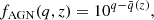
where q is the qTIR measured for our galaxy and  is the same quantity expected for a galaxy at the same redshift following the relation by Delhaize et al. (2017). Since in that study the qTIR(z) relation is found to have an intrinsic scatter of 0.26, we assign a fAGN = 0 to all the sources with
  (i.e., those compatible within 1σ with the relation expected for star-forming galaxies).
As visible in Figure 4, most of the galaxies in our sample have low values of the AGN fraction (fAGN < 0.3), and just 13 sources (∼10% of the full sample) are dominated by the AGN emission (fAGN > 0.9; see e.g., Enia et al. 2022) and – therefore – are removed from the sample. For all the other sources, we can account for the AGN contribution by computing the radio luminosity due to star formation as

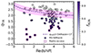 |
Fig. 4. Our estimation of the qTIR parameter for our galaxies as a function of the redshift. The dashed line reports the qTIR(z) relation by Delhaize et al. (2017), with the shaded area indicating the intrinsic scatter of the relation. Our galaxies are color-coded for their AGN fraction, measuring the contribution of nuclear activity to the radio luminosity. Galaxies classified as “radio-excess” (i.e., with fAGN > 0.9) are surrounded by a red square and removed from the sample. |
This value is then used to compute the SFR following Novak et al. (2017) as
![$$ \begin{aligned} \mathrm{SFR}[M_\odot \,\mathrm{yr}^{-1}] = 10^{-24} 10^{q(z)} \frac{L_{1.4\,\mathrm{GHz}}}{\mathrm{W\,Hz}^{-1}}, \end{aligned} $$](/articles/aa/full_html/2025/05/aa52461-24/aa52461-24-eq8.gif)
by assuming the same qTIR(z) relation found by Delhaize et al. (2017) and presented in Equation (3). As an additional test, we crossmatch our sample with the two publicly available X-ray catalogs of the COSMOS field (from the C-COSMOS and COSMOS Legacy surveys: Elvis et al. 2009; Civano et al. 2016) using as matching radius the positional uncertainties reported in there. We find a single source (cid_1076) with a counterpart in our sample. Given the relatively shallow depth of the X-ray observations in COSMOS, a detected source should have an X-ray luminosity higher than Lx > 1042 erg s−1 (more precisely, Lx ∼ 1044 erg s−1 in the range 2–10 keV assuming the photo-z by Cigale of z ∼ 3.5), likely hosting an un-obscured AGN. For this reason, we do not include this source in the rest of our analysis.
4. Luminosity function
4.1. Estimation of the luminosity function
We compute the luminosity function of our RS-NIR-faint galaxies by dividing our sample in three equally populated redshift bins, covering the ranges 2.5–3.3, 3.3–3.8, and 3.8–5.5. In each redshift bin, we divide the galaxies in several bins of (AGN-corrected) radio luminosity with a fixed width of 0.35 dex. To better sample the range of luminosities we employ bins that are overlapping by half of their width. In each combined redshift-luminosity bin, we compute the luminosity function following the 1/Vmax method (Schmidt 1968) as
where Δlog L is the log-amplitude of the luminosity bin and the sum extends to all the galaxies in that bin. For each galaxy, Vmax is computed as
![$$ \begin{aligned} V_{\rm max}=\sum _{z=z_{\rm min}}^{z_{\rm max}}[V(z+\Delta z)- V(z)]\, C(z), \end{aligned} $$](/articles/aa/full_html/2025/05/aa52461-24/aa52461-24-eq10.gif)
where we employ a fixed width of the redshift shells of Δz = 0.05. The C(z) term is the completeness function, and it can be written as the product of two terms:

The first one accounts for the limited area covered by the COSMOS-Web survey. In our case, it can be written as the ratio between the area of the survey and that of the whole sky:
The second term accounts for the incompleteness of the radio survey where our galaxies are selected. The completeness function of the 3 GHz survey performed during the VLA-COSMOS large program is reported in Smolčić et al. (2017) for resolved and un-resolved sources. Since in our sample we have both kinds of sources, for each flux we consider the average between the two values.
The sum in Equation (8) extends between two values zmin and zmax indicating the minimum and maximum redshift in which our target would be included in our sample according to our selection criteria. As described in Section 2.3, our galaxies need to have a radio S/N > 5 at 3 GHz and be faint in the F150W filter of NIRCam3.
As shown in Figure 5, these properties are affected by the redshift of each object: at higher redshifts, our galaxy becomes fainter in the radio, up to a certain z3 GHz where it becomes too faint to satisfy our S/N cut. Similarly, moving from high to low redshift, the F150W filter starts to sample less dust-obscured region of the SED, until a certain zNIR where the galaxy becomes too bright to satisfy our magnitude cut (F150W > 26.1 mag). Both these effects are accounted for in the definition of zmin and zmax as
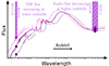 |
Fig. 5. Sketch showing the physical meaning of the zmin and zmax values employed in the estimation of the LF. These values account for the redshift range in which each target could be found according to our selection criteria. See the definitions of zNIR and z3 GHz in Section 4.1. |
where zmin, bin and zmax, bin indicate the lower and upper limits of the considered redshift bin. The values zNIR and z3 GHz are estimated for each galaxy by redshifting the best-fitting rest-frame SED on a grid with a step of Δz = 0.01 and measuring the expected fluxes at 3 GHz and in F150W filter of NIRCam at each redshift.
To account for the uncertainties in the photo-z and radio fluxes at 3 GHz of our sources, we perform a Monte-Carlo integration by extracting 5000 random values from the probability distributions of these quantities. For the redshifts, we directly sample the Gaussianized p(z) computed by Cigale, while for the radio fluxes we extract values from a Gaussian distribution centered on the mean value of the radio flux of each source and standard deviation equal to the related uncertainty. The value of the LF in each bin of redshift and radio luminosity is computed as the median value of all the iterations. Similarly, we assume as the upper and lower uncertainties the 16th and 84th percentiles, respectively. To account for the likely underestimation of the uncertainties in the less populated bins – due to the contribution of Poissonian uncertainties affecting low number counts – we correct these values in the bins with less than five galaxies with the 1σ confidence intervals reported in Gehrels (1986). Finally, we underline that our uncertainties do not include any contribution from cosmic variance. The values of the radio LF and the relative uncertainties are shown in Figure 6.
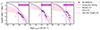 |
Fig. 6. Radio luminosity function at 3 GHz of our RS-NIR-faint galaxies. The points show the values computed as described in Section 4.1, while the dashed vertical lines indicate the minimum radio luminosity observable in a given redshift bin given the sensitivity of our survey. All the points corresponding to fainter luminosities (shaded points) are not included in the fitting. The shaded areas report the fitting of the modified Schechter function, with its 1 σ uncertainty. For reference, we also report the radio luminosity function (converted to 3 GHz by assuming a standard radio slope of α = −0.7) estimated by Novak et al. (2017), Enia et al. (2022), and van der Vlugt et al. (2022) on their samples of radio NIR-bright galaxies. |
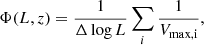
4.2. Modified Schechter function
In each redshift bin, we fit the LF of our sources with a modified Schechter function (Saunders et al. 1990), a common choice for radio and (sub)millimeter luminosity functions (see e.g., Novak et al. 2017; Gruppioni et al. 2020; Enia et al. 2022; van der Vlugt et al. 2022; Traina et al. 2024):
![$$ \begin{aligned} \Phi (L)=\Phi _\star \left(\frac{L}{L_\star }\right)^{1-\alpha }\mathrm{exp}\left[-\frac{1}{2\sigma ^2}\log ^2\left(1+\frac{L}{L_\star }\right)\right]. \end{aligned} $$](/articles/aa/full_html/2025/05/aa52461-24/aa52461-24-eq14.gif)
Due to the limited number of data-points available for fitting and the lack of constraints on the faint-end of the LF, we fix the two slope factors (α and σ) to the values found by Novak et al. (2017) in their analysis of the sample of radio sources (with optical/NIR counterparts) in the VLA-COSMOS large program. These values are σ = 0.63 and α = 1.22. We underline that the latter value is also in agreement with that found by van der Vlugt et al. (2022) in the deeper COSMOS-XS survey, better sampling the faint end of the radio LF. Possible caveats related to this choice are discussed in Section 5.2.
We fit the two remaining free parameters (Φ⋆ and L⋆, giving the normalization and the “knee” of the LF, respectively) with a Monte-Carlo Markov Chain (MCMC) performed with the Python library emcee (Foreman-Mackey et al. 2013). We adopt a flat prior on the two parameters: log(Φ⋆)∈[−6, −2] Mpc−3 dex−1 and log(L⋆)∈[20, 26] W Hz−1. We only include in the fitting procedure the points with L > Lmin, where Lmin represents the minimum radio luminosity observable in a redshift bin given the 5σ sensitivity of our radio survey. Moreover, since the LF is computed in overlapping bins of radio luminosity, we only include in the fitting half of the data-points to obtain un-correlated uncertainties.
The best-fitting parameters of the modified Schechter function – for each redshift bin – are reported in Table 2, while the fitted function (with its 1σ confidence interval) is reported as the shaded pink area in Figure 6.
Best-fitting parameters of the modified Schechter function fitted to our radio luminosity function at 3 GHz.
5. Contribution to the cosmic SFRD
In each redshift bin, we compute the contribution of the RS-NIR-faint galaxies to the total cosmic SFRD by integrating the analytic expression of the modified Schechter function weighted for the SFR related to each radio luminosity:
where SFR(L, z) is the expression reported in Equation (6) and z is the mean redshift of each bin. In this integral, we consider the full posterior distribution of the parameters in the modified Schechter function obtained from the MCMC in Section 4.2 in order to compute the uncertainties on the SFRD.
We perform two different integrals. The first one only includes the radio luminosities between the Lmin related to the sensitivity of our radio survey and the maximum luminosity observed in each redshfit bin. The second extends over the full range of radio luminosities (0 → +∞). While the first integral estimates the contribution of the galaxies that are actually observed in our surveys to the cosmic SFRD, the second one includes in this estimates the galaxies that are not observed in our survey but that we expect by extrapolating the radio LF at higher and lower luminosities. We underline that – given these definitions – the first value should be interpreted as a lower limit on the actual contribution of the RS-NIR-faint galaxies to the cosmic SFRD. The results of these integrals are summarized in Table 3 and in Figure 7. It is possible to notice how our estimates have large uncertainties. The reason for this can be found in the lack of strong constraints on the L⋆ parameter of the LF. Being our galaxies unable to trace the faint end of the LF, our analysis can only pose a robust upper limit on the location of the “knee”. Deeper radio data would be needed to better constrain this value (and, consequently, the contribution to the SFRD).
Contribution of the RS-NIR-faint galaxies to the cosmic SFRD.
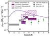 |
Fig. 7. Cosmic SFRD. The values obtained by integrating the luminosity function of our RS-NIR-faint galaxies are reported in purple. The values obtained by integrating the observed range of luminosities are shown with full squares, while the empty boxes report the values obtained by integrating the LF on the full range of radio luminosities. The figure shows, for reference, the SFRD computed by Madau & Dickinson (2014) on “optically bright” galaxies (dashed indigo line), and those obtained by Behiri et al. (2023), van der Vlugt et al. (2023), Enia et al. (2022), and Barrufet et al. (2023) (grey boxes, purple diamond, grey points, and green squares, respectively) for their “NIR-faint galaxies” selected in the radio and with JWST. |
5.1. Contribution of radio-selected NIR-faint galaxies to the cosmic SFRD
The results obtained in Section 5 indicate an increasing contribution of the RS-NIR-faint galaxies to the cosmic SFRD from z ∼ 3 to z ∼ 3.5 and then decreasing until z ∼ 4.5. This result agrees with previous studies focusing on NIRdark/faint radio sources at z > 2.5. Our “observed” results are consistent (even though moderately lower at z ∼ 3) with those obtained by Behiri et al. (2023), analyzing the same kind of sources in the COSMOS field (even though with a slightly different selection, see Section 2.3). In that study, no extrapolation was performed outside the observed range of luminosities. Therefore it is not surprising that our “extrapolated” results are significantly higher. Similarly, our estimation of the SFRD at z ∼ 3 agrees well with the lower limit presented in Enia et al. (2022) when no extrapolation is performed.
Our “extrapolated” results can be compared with the upper limit provided by Enia et al. (2022) (analyzing NIRdark galaxies in the GOODS-N field) and with the estimates by van der Vlugt et al. (2023) (analyzing analogous sources in the deep COSMOS-XS survey). Both these studies estimated the radio LF and computed the contribution to the cosmic SFRD by integrating it in the full range of radio luminosities (0 → ∞). It is important to notice, however, that the three studies estimate the contribution to the total SFRD in different ways. The other two studies, indeed, focused on smaller fields compared with COSMOS-Web (0.05 deg2 in GOODS-N and 0.1 deg2 in COSMOS-XS, instead of the 0.54 deg2 covered by our survey). This difference produced significantly smaller samples of NIRdark galaxies available for the analysis (nine sources for Enia et al. 2022 and 20 for van der Vlugt et al. 2023, against the ∼120 analysed here). To overcome this issue, Enia et al. (2022) fixed three parameters in the Schechter fitting of the LF (σ, α, and L⋆) to those obtained for the NIR-bright population, leaving only the normalization (Φ⋆) as a free parameter of the fitting. Likewise, van der Vlugt et al. (2023) computed the LF on the full sample of radio sources twice: once including the NIRdark galaxies and once excluding them: the contribution of these sources was then found by subtracting the two inferred SFRDs.
Our results at z ∼ 3.5 agree well with the upper limit at the same redshift by Enia et al. (2022). Similarly, our result in the highest redshift bin (z ∼ 4.5) is compatible with the estimate by van der Vlugt et al. (2023). Their results are more in tension with ours at z ∼ 3 and z ∼ 3.5, with our estimates being up to one order of magnitude higher. A possible explanation of this discrepancy could reside in the accuracy of the photo-z (our photometry includes the new NIRCam and MIRI photometry, that could result in more accurate redshift estimates; see e.g., Barrufet et al. 2025).
5.2. Possible caveats of our analysis
Our analysis is not immune to possible biases. The most common one is an inaccuracy in the photometric redshifts estimated through SED fitting. Even with the new constraints obtained thanks to NIRCam and MIRI, the small number of photometric detections and the large number of upper limits make our estimates uncertain. We reduced the possible impact of this issue on our results by employing in our analysis the full Gaussianized p(z) given in output by Cigale, resulting in larger uncertainties on our LF and SFRD. This issue could be solved in the future with a spectroscopic follow-up of our galaxies (analogous to that performed by Barrufet et al. 2025 with JWST, or those performed by Jin et al. 2019, 2022; Chen et al. 2022; Gentile et al. 2024c with ALMA).
Another caveat (more related to our radio selection) resides in the possible AGN contribution not unveiled by our qTIR analysis. An overestimated radio luminosity due to star-formation could still bias our LF and SFR, producing a different behavior of the SFRD. This issue can be partially solved with a more complete photometric coverage at MIR wavelengths, where the thermal emission of a hot dusty torus surrounding the AGN should be visible (see e.g., Hickox & Alexander 2018 for a review and Chien et al. 2024 for a recent application with MIRI data).
Finally, our analysis (especially the “extrapolated” value of the SFRD) relies on a strong assumption about the shape of the LF. In our fitting procedure, we fixed the two parameters of the modified Schechter function α and σ to those obtained by Novak et al. (2017) for their sample of radio sources in the COSMOS field (i.e., the parent sample of our selection). This choice, however, assumes that the selection of more dust-obscured sources is not altering these parameters. This assumption could be incorrect, since we expect the number of NIR-faint sources to be lower in the low-SFR regime (e.g., for a lower production of dust from supernovae) and higher in the high-SFR one (see e.g., Whitaker et al. 2017 and Traina et al., in prep.). This issue could be improved with a deeper radio survey (e.g., van der Vlugt et al. 2022) giving us more information about the faint-end slope of the LF for our sources.
6. Discussion
6.1. Effect of NIR-faint selection
To interpret the results presented in the previous sections, it is useful to compare our population of galaxies with other samples studied in the current literature. The first one is the total population of radio-detected sources, of which the RS-NIR-faint galaxies are a sub-population with F150W > 26.1 mag. One of the main results of this comparison is shown in Figure 2, where we report the photo-z estimated for our galaxies and those computed by Shuntov, Paquereau et al. (in prep.) for the other 3 GHz sources in the COMSOS-Web survey with F150W > 26.1 mag. It is immediately possible to see that our galaxies are – on average – located at higher redshifts with respect to the rest of the population. An analogous result has been shown by van der Vlugt et al. (2023) for their NIRdark galaxies selected in the deep radio survey COSMOS-XS and by Talia et al. (2021) and Behiri et al. (2023) in their previous analysis of RS-NIRdark galaxies in the COSMOS field. The same idea that NIR-faint DSFGs represent the high-redshift end of their parent distributions is also present in other studies selecting DSFGs at other wavelengths (see e.g., the studies on NIR-faint sub-millimeter galaxies by Simpson et al. 2014; Franco et al. 2018; Smail et al. 2021; McKinney et al. 2025). This result is likely connected to the existence of the zNIR introduced in Section 4.1 (see also Figure 5) directly arising from the requirement of faintness at NIR wavelengths.
The different distribution of the photo-z also affects the estimated luminosity functions. Here, we consider those by Novak et al. (2017), Enia et al. (2022), and van der Vlugt et al. (2022) focusing on NIR-bright galaxies. These estimates are reported for reference in Figure 6, while the best-fitting parameters of the modified Schechter function found by Enia et al. (2022) are reported in Table 2. It is possible to notice how the normalization of the luminosity function for our NIR-faint galaxies is on average ∼1.5 − 2 dex lower than what is observed for optically bright sources. The luminosity of the knee, instead, seems to be higher for our sources, even though compatible with the values from Enia et al. (2022) within the (large) uncertainties.
The first result is not unexpected, since we are dealing with a population of heavily dust-obscured sources less common than NIR-bright galaxies (see e.g., the comparison between the number of 3 GHz sources in COSMOS-Web and those in our sample in Section 2). The second result is more interesting, since it suggests that the high dust obscuration could positively correlate with the radio luminosity (and – therefore – with the SFR). This result is not completely new, since several previous studies (e.g., Whitaker et al. 2017 and Traina et al., in prep.) highlighted how the dust-obscured star formation could dominate the high-SFR end of the star formation rate function, at least until the cosmic noon. The main consequence of the higher turn-off luminosity can be seen in Figure 6, where is visible how the NIR-faint galaxies could dominate the LF in its bright end (even though, again, still compatible in most cases within the estimated uncertainties). The higher volume densities of our sources in the bright end also explains the large contribution to the SFRD when we integrate the LF on the whole range of radio luminosities to compute the SFRD (Figure 7).
6.2. Effect of radio selection
Once confirmed that the radio selection is able to produce a sample of DSFGs, we want to analyse how this method compares with analogous strategies present in the current literature. In this section, we will focus on two main approaches: the selection by Barrufet et al. (2023) and Gottumukkala et al. (2024) based on the JWST colors, and that by McKinney et al. (2025) based on the (sub)millimeter detection.
6.2.1. JWST-selected DSFGs
We firstly compare our sources with those collected by Barrufet et al. (2023) and Gottumukkala et al. (2024) in the Cosmic Evolution Early Release Science (CEERS; Finkelstein et al. 2023). These studies mimic the DSFG selection initially performed by Wang et al. (2019) with the so-called “H-dropout” (i.e., galaxies selected through their H - [4.5] colors) by taking advantage of the new JWST photometry. More in detail, this selection couples the F150W–F444W > 2.1 mag color cut with a magnitude cut in the F150W filter (F150W > 25.0 mag in Gottumukkala et al. 2024). As visible in Figure 8, our RS-NIR-faint galaxies represent a sub-sample of the sources analysed by Gottumukkala et al. (2024), satisfying – by construction – the same criteria about faintness in F150W, having comparable F150W–F444W colors, but with the additional requirement of the radio detection. By comparing these samples, we can study how the radio selection affects the retrieved population of galaxies. Since the selection by Gottumukkala et al. (2024) includes fainter sources in the F150W filter, in the following we will focus on their sources satisfying our F150W > 26.1 criterion.
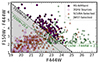 |
Fig. 8. Our RS-NIR-faint galaxies in the F150W-F444W versus F444W color-magnitude plot. We report, for comparison, the JWST-selected DSFGs by Gottumukkala et al. (2024) and the SCUBA-selected ones by McKinney et al. (2025). Even if we do not pose any constrain in the F150W-F444W color, we obtain that all our sources are above the threshold adopted by Gottumukkala et al. (2024), identifying our galaxies as a sub-population of the JWST-selected DSFGs. Similarly, part of the SCUBA-selected DSFGs satisfy our “NIR-faint” criterion. |
The first notable difference is in the projected sky density of the two populations 6000 ± 77 deg−2 for the sources by Gottumukkala et al. (2024) and 205 ± 14 deg−24 for our RS-NIR-faint galaxies. Then, by looking at the physical properties summarized in Figure 3, we can see that the distributions of the photo-z are quite similar until z ∼ 4, but with different behavior at higher redshifts. This result is not surprising given the much stronger k-correction in the radio than in the F444W filter of NIRCam (see e.g., the shape of the SEDs in Figure 1), biasing our sample towards lower-z sources.
Another notable difference consists in the reported values of SFR. As visible in Figure 3, our RS-NIR-faint galaxies are ∼1.5 dex more star-forming than the sources analysed by Barrufet et al. (2023) and Gottumukkala et al. (2024). On the one hand, this result is not surprising since the need for a radio detection excludes from our sample all the objects with low values of SFR. As noted by Wang et al. (2019) and verified by Barrufet et al. (2025) with a spectroscopic follow-up of some JWST-selected objects, the red NIRCam colors alone are not enough to select DSFGs, since the same colors can be seen in quiescent galaxies. This ambiguity in the true nature of these sources can be solved with additional data from JWST (mainly spectra, as in Barrufet et al. 2025), or a more complete MIRI coverage (as in Pérez-González et al. 2023), ALMA (as in Wang et al. 2019) or in the radio regime (as for our sources).
If the radio selection well explains why our sample lacks low-SFR galaxies, it does not explain why the high-SFR sources are not present in the sample by Gottumukkala et al. (2024). A possible explanation resides in the photometric coverage of their sample. At the redshifts covered by their observations, no constraints on the rest-frame UV is available for the SED fitting, making quite uncertain the value of the SFR obtained through it. Similarly, we expect most of the star formation in these NIR-faint galaxies to be dust-obscured and – therefore – hard to constrain without some information on the FIR or radio emission, producing a likely underestimation of the SFR (see, e.g., some examples in Xiao et al. 2024).
The higher values of the SFR also explain one of the results visible in Figure 7: even though the RS-NIR-faint galaxies are ∼1.5 dex less common than the JWST-selected sources, the higher values of SFR (∼1.5 dex) still produce compatible contribution to the cosmic SFRD for the “observed” sources. The values obtained by extrapolating at higher and lower radio luminosities are obviously higher than those reported by Barrufet et al. (2023), since their estimate only accounts for the detected sources.
6.2.2. SCUBA-selected DSFGs
Together with the MIR- and radio-based selections, another possibility to select DSFGs relies on the detection at (sub)millimeter wavelengths of the bright thermal emission by warm dust heated by ongoing star formation (see e.g., Casey et al. 2014, for a review). Galaxies selected through this procedure are commonly known as sub-millimeter galaxies (SMGs). Since this definition strongly relies on the depth of the observations employed to select these objects, in this study we only focus on the sources described in McKinney et al. (2025), acknowledging that some differences might arise when other samples (detected in deeper or shallower surveys; see e.g., da Cunha et al. 2015; Dudzevičiūtė et al. 2021) are considered. These 289 galaxies were initially selected in the COSMOS field as sources with S870 μm > 2 mJy in the SCUBA-2 observations performed during the S2COSMOS survey (Simpson et al. 2019) and then followed-up with ALMA (unveiling in some cases the presence of multiple fainter sources contributing to the total flux of the SCUBA-2 objects). The SCUBA-Dive program described in McKinney et al. (2025) performs a deeper analysis of these sources taking advantage of the new JWST data coming from the COSMOS-Web survey.
Looking at the color-magnitude plot in Figure 8, we can note only a partial overlap between the SCUBA-selected galaxies and our RS-NIR-faint ones, since most of the former are brighter (i.e., not NIR-faint) in the F150W filter. Since both samples are selected in the COSMOS field, we can crossmatch the two catalogs, finding only a partial overlap of 27 objects. We underline that the SCUBA-Dive programs only focuses on the SCUBA-2 sources with previous ALMA data. Therefore some of our galaxies could still be included in that sample with additional data. To overcome this issue, we analyze the best-fitting SEDs computed with Cigale for our galaxies, obtaining that only 82 (∼65%) of our sources would have a S850 μm > 2 mJy, being consistent with the initial cut employed on the SCUBA-2 maps by McKinney et al. (2025).
By comparing the physical properties estimated through SED fitting (Figure 3), we can see that the distributions of stellar masses and SFR are quite similar. More significant differences hold for the photo-z (with our galaxies located – on average – at higher redshifts: ⟨z⟩∼3.6 for our sources and ⟨z⟩∼2.6 for those in SCUBA-Dive) and for the dust attenuation (with our sources being – on average – more dust-obscured; ⟨Av⟩∼3.5 mag against ⟨Av⟩∼2.5 mag). Both results are easily explained by the NIR-faint selection, biasing the sample towards more dust-obscured and higher-z objects (see also the discussion in Section 6.1).
A further confirmation of this result can be found in the comparison with the SCUBA-Dive sources satisfying the same magnitude cut as our RS-NIR-faint galaxies (F150W > 26.1 mag). As visible from Figure 3, these sources have analogous properties to our galaxies, indicating that the two selections are able to identify the same population of objects with different procedures.
7. Summary
In this paper, we presented the first analysis taking advantage of JWST data of radio-selected NIR-faint sources in the COSMOS field. These sources are defined as radio-detected sources with a counterpart at NIR wavelengths (unveiled with the deep NIRCam observations) fainter than the common depths reached by ground-based facilities. We obtained the following results:
-
The physical properties estimated through SED fitting indicate that the RS-NIR-faint galaxies are a population of highly dust-obscured (⟨Av⟩∼3.5 mag), massive (⟨M⋆⟩∼1010.8 M⊙) and star-forming galaxies (⟨SFR⟩∼300 M⊙ yr−1) located at ⟨z⟩∼3.6.
-
Estimating the radio luminosity function of our sources and fitting it with a modified Schechter function, we find that its normalization (Φ⋆) is ∼1.5−2 dex lower than that computed on radio-selected NIR-bright galaxies (e.g., Novak et al. 2017; Enia et al. 2022; van der Vlugt et al. 2022), indicating that – as expected – DSFGs with faint optical/NIR counterparts are a rare population.
-
Interestingly, the knee of the radio LF for our sources is brighter than for NIR-bright sources (even though compatible within the large estimated uncertainties). This result suggests that the fractional contribution of RS-NIR-faint sources (with respect to the overall population of galaxies at a given radio luminosity) is negligible in the low-SFR end of the star formation rate function, while it becomes dominant in the high-SFR end, at least until z ∼ 4.5. This result confirms what has been found in previous studies focusing on the ratio between obscured and unobscured star formation in high-z galaxies.
-
By integrating the LF of our sources in the range of radio luminosities covered by our observations, we put a lower limit on their contribution to the cosmic SFRD. Our result shows an increasing contribution from z ∼ 3 to z ∼ 3.5 and then decreasing until z ∼ 4.5.
-
By integrating the LF in the full range of radio luminosities (0 → ∞; i.e., extrapolating at higher and lower radio luminosities than what is actually observed), we increase the contribution to the total cosmic SFRD, reaching the same level of the NIR-bright galaxies analysed by Madau & Dickinson (2014).
-
When compared with the JWST selection of DSFGs carried out by Barrufet et al. (2023) and Gottumukkala et al. (2024), we obtain that our radio selection generally misses the sources located at higher redshifts (z > 5.5), as expected given the positive k-correction affecting the radio emission. Moreover, our sources are ∼1.5 dex more rare, and ∼1.5 dex more star-forming. The main consequence of these differences, is that their contribution to the cosmic SFRD (not extrapolating at higher and lower radio luminosities) is compatible with that estimated by Barrufet et al. (2023) up to z ∼ 5.
-
Finally, we compare our sources with the SCUBA-selected ones found in the COSMOS-Web survey by McKinney et al. (2025), obtaining that our galaxies have analogous properties to their sources in terms of stellar mass and SFR. Our RS-NIR-faint galaxies are – on average – located at higher redshifts and more dust-obscured, as expected for our requirement about the faintness at NIR wavelengths. Comparing our sources with the SCUBA-selected galaxies satisfying the same F150W > 26.1 mag requirement, we obtain more similar distributions of photo-z and Av.
These results together justify the scientific interest in the population of RS-NIR-faint galaxies, picturing this selection as an efficient way of assembly statistically significant DSFGs in wide radio surveys.
The same lack of constraints in the rest-UV affects, in theory, also the estimation of Av. Nevertheless, since we have some constrains from the rest-optical and from the employment of an SED-fitting code relying on the energy balance, we decide to still report our estimate of Av in Table 1.
We underline that the analysis described in Delhaize et al. (2017) is based on the same radio survey employed to select the galaxies in this study.

Acknowledgments
We warmly thank the anonymous referee for his/her comments on the first version of this paper, which really allowed us to increase the overall quality of our study. F.G. thanks the department of astronomy of the University of Texas at Austin for the hospitality during the initial writing of this paper. F.G., M.T., and A. C. acknowledge the support from grant PRIN MIUR 2017-20173ML3WW_001. ‘Opening the ALMA window on the cosmic evolution of gas, stars, and supermassive black holes’. MF acknowledges funding from the European Union’s Horizon 2020 research and innovation programme under the Marie Sklodowska-Curie grant agreement No 101148925. The french members of the COSMOS team acknowledge the support from CNES. The Cosmic Dawn Center (DAWN) is funded by the Danish National Research Foundation under grant DNRF140. M. V. acknowledges financial support from the Inter-University Institute for Data Intensive Astronomy (IDIA), a partnership of the University of Cape Town, the University of Pretoria and the University of the Western Cape, and from the South African Department of Science and Innovation’s National Research Foundation under the ISARP RADIOMAP Joint Research Scheme (DSI-NRF Grant Number 150551) and the CPRR HIPPO Project (DSI-NRF Grant Number SRUG22031677). The Flatiron Institute is supported by the Simons Foundation. The data described here may be obtained from http://dx.doi.org/10.17909/h9k1-dc06
References
- Adscheid, S., Magnelli, B., Liu, D., et al. 2024, A&A, 685, A1 [NASA ADS] [CrossRef] [EDP Sciences] [Google Scholar]
- Aihara, H., AlSayyad, Y., Ando, M., et al. 2019, PASJ, 71, 114 [Google Scholar]
- Barrufet, L., Oesch, P. A., Weibel, A., et al. 2023, MNRAS, 522, 449 [NASA ADS] [CrossRef] [Google Scholar]
- Barrufet, L., Oesch, P. A., Marques-Chaves, R., et al. 2025, MNRAS, submitted [arXiv:2404.08052] [Google Scholar]
- Behiri, M., Talia, M., Cimatti, A., et al. 2023, ApJ, 957, 63 [NASA ADS] [CrossRef] [Google Scholar]
- Bertin, E., Schefer, M., Apostolakos, N., et al. 2020, The SourceXtractor++ Software (San Francisco: Astronomical Society of the Pacific), 461 [Google Scholar]
- Boquien, M., Burgarella, D., Roehlly, Y., et al. 2019, A&A, 622, A103 [NASA ADS] [CrossRef] [EDP Sciences] [Google Scholar]
- Bruzual, G., & Charlot, S. 2003, MNRAS, 344, 1000 [NASA ADS] [CrossRef] [Google Scholar]
- Burgarella, D., Buat, V., Gruppioni, C., et al. 2013, A&A, 554, A70 [NASA ADS] [CrossRef] [EDP Sciences] [Google Scholar]
- Casey, C. M., Narayanan, D., & Cooray, A. 2014, Phys. Rep., 541, 45 [Google Scholar]
- Casey, C. M., Zavala, J. A., Manning, S. M., et al. 2021, ApJ, 923, 215 [NASA ADS] [CrossRef] [Google Scholar]
- Casey, C. M., Kartaltepe, J. S., Drakos, N. E., et al. 2023, ApJ, 954, 31 [NASA ADS] [CrossRef] [Google Scholar]
- Ceraj, L., Smolčić, V., Delvecchio, I., et al. 2018, A&A, 620, A192 [NASA ADS] [CrossRef] [EDP Sciences] [Google Scholar]
- Chabrier, G. 2003, PASP, 115, 763 [Google Scholar]
- Chapman, S. C., Richards, E. A., Lewis, G. F., Wilson, G., & Barger, A. J. 2001, ApJ, 548, L147 [NASA ADS] [CrossRef] [Google Scholar]
- Charlot, S., & Fall, S. M. 2000, ApJ, 539, 718 [Google Scholar]
- Chen, C.-C., Liao, C.-L., Smail, I., et al. 2022, ApJ, 929, 159 [NASA ADS] [CrossRef] [Google Scholar]
- Chien, T. C. C., Ling, C.-T., Goto, T., et al. 2024, MNRAS, 532, 719 [Google Scholar]
- Civano, F., Marchesi, S., Comastri, A., et al. 2016, ApJ, 819, 62 [Google Scholar]
- Cochrane, R. K., Anglés-Alcázar, D., Cullen, F., & Hayward, C. C. 2024, ApJ, 961, 37 [NASA ADS] [CrossRef] [Google Scholar]
- da Cunha, E., Walter, F., Smail, I. R., et al. 2015, ApJ, 806, 110 [Google Scholar]
- Delhaize, J., Smolčić, V., Delvecchio, I., et al. 2017, A&A, 602, A4 [NASA ADS] [CrossRef] [EDP Sciences] [Google Scholar]
- Dempsey, J. T., Friberg, P., Jenness, T., et al. 2013, MNRAS, 430, 2534 [Google Scholar]
- Draine, B. T., Aniano, G., Krause, O., et al. 2014, ApJ, 780, 172 [Google Scholar]
- Dudzevičiūtė, U., Smail, I., Swinbank, A. M., et al. 2021, MNRAS, 500, 942 [Google Scholar]
- Elvis, M., Civano, F., Vignali, C., et al. 2009, ApJS, 184, 158 [Google Scholar]
- Enia, A., Talia, M., Pozzi, F., et al. 2022, ApJ, 927, 204 [NASA ADS] [CrossRef] [Google Scholar]
- Euclid Collaboration (Moneti, A., et al.) 2022, A&A, 658, A126 [NASA ADS] [CrossRef] [EDP Sciences] [Google Scholar]
- Ferland, G. J., Porter, R. L., van Hoof, P. A. M., et al. 2013, Rev. Mex. Astron. Astrofis., 49, 137 [Google Scholar]
- Finkelstein, S. L., Bagley, M. B., Ferguson, H. C., et al. 2023, ApJ, 946, L13 [NASA ADS] [CrossRef] [Google Scholar]
- Foreman-Mackey, D., Hogg, D. W., Lang, D., & Goodman, J. 2013, PASP, 125, 306 [Google Scholar]
- Franco, M., Elbaz, D., Béthermin, M., et al. 2018, A&A, 620, A152 [NASA ADS] [CrossRef] [EDP Sciences] [Google Scholar]
- Gehrels, N. 1986, ApJ, 303, 336 [Google Scholar]
- Gentile, F., Talia, M., Behiri, M., et al. 2024a, ApJ, 962, 26 [NASA ADS] [CrossRef] [Google Scholar]
- Gentile, F., Casey, C. M., Akins, H. B., et al. 2024b, ApJ, 973, L2 [NASA ADS] [CrossRef] [Google Scholar]
- Gentile, F., Talia, M., Daddi, E., et al. 2024c, A&A, 687, A288 [NASA ADS] [CrossRef] [EDP Sciences] [Google Scholar]
- Gillman, S., Smail, I., Gullberg, B., et al. 2024, A&A, 691, A299 [NASA ADS] [CrossRef] [EDP Sciences] [Google Scholar]
- Gottumukkala, R., Barrufet, L., Oesch, P. A., et al. 2024, MNRAS, 530, 966 [NASA ADS] [CrossRef] [Google Scholar]
- Gruppioni, C., Pozzi, F., Rodighiero, G., et al. 2013, MNRAS, 432, 23 [Google Scholar]
- Gruppioni, C., Béthermin, M., Loiacono, F., et al. 2020, A&A, 643, A8 [NASA ADS] [CrossRef] [EDP Sciences] [Google Scholar]
- Hickox, R. C., & Alexander, D. M. 2018, ARA&A, 56, 625 [Google Scholar]
- Hodge, J. A., da Cunha, E., Kendrew, S., et al. 2025, ApJ, 978, 165 [NASA ADS] [CrossRef] [Google Scholar]
- Hughes, D. H., Serjeant, S., Dunlop, J., et al. 1998, Nature, 394, 241 [Google Scholar]
- Jarvis, M., Taylor, R., Agudo, I., et al. 2016, in MeerKAT Science: On the Pathway to the SKA, 6 [Google Scholar]
- Jin, S., Daddi, E., Liu, D., et al. 2018, ApJ, 864, 56 [Google Scholar]
- Jin, S., Daddi, E., Magdis, G. E., et al. 2019, ApJ, 887, 144 [Google Scholar]
- Jin, S., Daddi, E., Magdis, G. E., et al. 2022, A&A, 665, A3 [NASA ADS] [CrossRef] [EDP Sciences] [Google Scholar]
- Kennicutt, R. C., & Evans, N. J. 2012, ARA&A, 50, 531 [NASA ADS] [CrossRef] [Google Scholar]
- Koekemoer, A. M., Aussel, H., Calzetti, D., et al. 2007, ApJS, 172, 196 [Google Scholar]
- Kümmel, M., Bertin, E., Schefer, M., et al. 2020, Working with the SourceXtractor++ Software (San Francisco: Astronomical Society of the Pacific), 29 [Google Scholar]
- Liu, D., Lang, P., Magnelli, B., et al. 2019, ApJS, 244, 40 [Google Scholar]
- Lutz, D., Poglitsch, A., Altieri, B., et al. 2011, A&A, 532, A90 [NASA ADS] [CrossRef] [EDP Sciences] [Google Scholar]
- Madau, P., & Dickinson, M. 2014, ARA&A, 52, 415 [Google Scholar]
- McCracken, H. J., Milvang-Jensen, B., Dunlop, J., et al. 2012, A&A, 544, A156 [NASA ADS] [CrossRef] [EDP Sciences] [Google Scholar]
- McKinney, J., Casey, C. M., Long, A. S., et al. 2025, ApJ, 979, 229 [Google Scholar]
- Novak, M., Smolčić, V., Delhaize, J., et al. 2017, A&A, 602, A5 [NASA ADS] [CrossRef] [EDP Sciences] [Google Scholar]
- Oke, J. B., & Gunn, J. E. 1983, ApJ, 266, 713 [NASA ADS] [CrossRef] [Google Scholar]
- Oliver, S. J., Bock, J., Altieri, B., et al. 2012, MNRAS, 424, 1614 [NASA ADS] [CrossRef] [Google Scholar]
- Pérez-González, P. G., Barro, G., Annunziatella, M., et al. 2023, ApJ, 946, L16 [CrossRef] [Google Scholar]
- Salim, S., & Narayanan, D. 2020, ARA&A, 58, 529 [NASA ADS] [CrossRef] [Google Scholar]
- Saunders, W., Rowan-Robinson, M., Lawrence, A., et al. 1990, MNRAS, 242, 318 [Google Scholar]
- Schinnerer, E., Smolčić, V., Carilli, C. L., et al. 2007, ApJS, 172, 46 [Google Scholar]
- Schmidt, M. 1968, ApJ, 151, 393 [Google Scholar]
- Scoville, N., Aussel, H., Brusa, M., et al. 2007, ApJS, 172, 1 [Google Scholar]
- Sérsic, J. L. 1963, Boletin de la Asociacion Argentina de Astronomia La Plata Argentina, 6, 41 [Google Scholar]
- Simpson, J. M., Swinbank, A. M., Smail, I., et al. 2014, ApJ, 788, 125 [Google Scholar]
- Simpson, J. M., Smail, I., Swinbank, A. M., et al. 2019, ApJ, 880, 43 [NASA ADS] [CrossRef] [Google Scholar]
- Smail, I., Ivison, R. J., & Blain, A. W. 1997, ApJ, 490, L5 [NASA ADS] [CrossRef] [Google Scholar]
- Smail, I., Owen, F. N., Morrison, G. E., et al. 2002, ApJ, 581, 844 [NASA ADS] [CrossRef] [Google Scholar]
- Smail, I., Dudzevičiūtė, U., Stach, S. M., et al. 2021, MNRAS, 502, 3426 [NASA ADS] [CrossRef] [Google Scholar]
- Smolčić, V., Novak, M., Bondi, M., et al. 2017, A&A, 602, A1 [Google Scholar]
- Swinyard, B. M., Ade, P., Baluteau, J. P., et al. 2010, A&A, 518, L4 [NASA ADS] [CrossRef] [EDP Sciences] [Google Scholar]
- Tadhunter, C. 2016, A&ARv, 24, 10 [Google Scholar]
- Talia, M., Cimatti, A., Giulietti, M., et al. 2021, ApJ, 909, 23 [NASA ADS] [CrossRef] [Google Scholar]
- Traina, A., Gruppioni, C., Delvecchio, I., et al. 2024, A&A, 681, A118 [NASA ADS] [CrossRef] [EDP Sciences] [Google Scholar]
- van der Vlugt, D., Hodge, J. A., Algera, H. S. B., et al. 2022, ApJ, 941, 10 [NASA ADS] [CrossRef] [Google Scholar]
- van der Vlugt, D., Hodge, J. A., Jin, S., et al. 2023, ApJ, 951, 131 [NASA ADS] [CrossRef] [Google Scholar]
- Wang, T., Schreiber, C., Elbaz, D., et al. 2019, Nature, 572, 211 [Google Scholar]
- Weaver, J. R., Kauffmann, O. B., Ilbert, O., et al. 2022, ApJS, 258, 11 [NASA ADS] [CrossRef] [Google Scholar]
- Whitaker, K. E., Pope, A., Cybulski, R., et al. 2017, ApJ, 850, 208 [NASA ADS] [CrossRef] [Google Scholar]
- Williams, C. C., Alberts, S., Ji, Z., et al. 2024, ApJ, 968, 34 [NASA ADS] [CrossRef] [Google Scholar]
- Xiao, M., Oesch, P. A., Elbaz, D., et al. 2024, Nature, 635, 311 [NASA ADS] [CrossRef] [Google Scholar]
Appendix A: Cigale parameters
In Table A.1 we report the modules and parameters employed in our SED-fitting setup with Cigale.
Parameters of the SED fitting performed with Cigale.
All Tables
Best-fitting parameters of the modified Schechter function fitted to our radio luminosity function at 3 GHz.
All Figures
|
Fig. 1. Some examples of the SED fitting performed with Cigale on the galaxies included in the highest redshift bin. The squares indicate the photometric points from JWST, A3COSMOS and the 870 μm from the deblending of the S2COSMOS maps by Simpson et al. (2019). The circular points report the ancillary photometry from HSC, VISTA, Spitzer, and from the super-deblending of the Herschel Maps. The inset shows the Gaussianized p(z) computed with Cigale. The top row shows the cutouts (3 arcsec side) in the NIRCam and MIRI filters of COSMOS-Web. |
| In the text | |
|
Fig. 2. Distribution of the photometric redshifts of our RS-NIR-faint galaxies in COSMOS-Web. Our sources are reported as the purple solid line, while the complementary sample of 3 GHz objects with F150W > 26.1 mag is reported as the blue solid line. For reference, we also show the photo-z computed by Enia et al. (2022) on their sample of radio sources (with optical/NIR counterparts) in the GOODS-N field (blue dashed line) and those estimated by van der Vlugt et al. (2023) for their sample of optically/NIR-faint galaxies in their deeper COSMOS-XS survey (dashed pink line). |
| In the text | |
|
Fig. 3. Main properties (photometric redshift, stellar mass, SFR, and dust extinction) of our RS-NIR-faint galaxies. We show – for comparison – the same properties computed by Gottumukkala et al. (2024) and McKinney et al. (2025) for their sample of JWST-selected and SCUBA-selected DSFGs as the green and orange solid lines, respectively. To allow a fair comparison, we only include the sources by Gottumukkala et al. (2024) with F150W > 26.1 mag and exclude the sources flagged as possible AGN. |
| In the text | |
|
Fig. 4. Our estimation of the qTIR parameter for our galaxies as a function of the redshift. The dashed line reports the qTIR(z) relation by Delhaize et al. (2017), with the shaded area indicating the intrinsic scatter of the relation. Our galaxies are color-coded for their AGN fraction, measuring the contribution of nuclear activity to the radio luminosity. Galaxies classified as “radio-excess” (i.e., with fAGN > 0.9) are surrounded by a red square and removed from the sample. |
| In the text | |
|
Fig. 5. Sketch showing the physical meaning of the zmin and zmax values employed in the estimation of the LF. These values account for the redshift range in which each target could be found according to our selection criteria. See the definitions of zNIR and z3 GHz in Section 4.1. |
| In the text | |
|
Fig. 6. Radio luminosity function at 3 GHz of our RS-NIR-faint galaxies. The points show the values computed as described in Section 4.1, while the dashed vertical lines indicate the minimum radio luminosity observable in a given redshift bin given the sensitivity of our survey. All the points corresponding to fainter luminosities (shaded points) are not included in the fitting. The shaded areas report the fitting of the modified Schechter function, with its 1 σ uncertainty. For reference, we also report the radio luminosity function (converted to 3 GHz by assuming a standard radio slope of α = −0.7) estimated by Novak et al. (2017), Enia et al. (2022), and van der Vlugt et al. (2022) on their samples of radio NIR-bright galaxies. |
| In the text | |
|
Fig. 7. Cosmic SFRD. The values obtained by integrating the luminosity function of our RS-NIR-faint galaxies are reported in purple. The values obtained by integrating the observed range of luminosities are shown with full squares, while the empty boxes report the values obtained by integrating the LF on the full range of radio luminosities. The figure shows, for reference, the SFRD computed by Madau & Dickinson (2014) on “optically bright” galaxies (dashed indigo line), and those obtained by Behiri et al. (2023), van der Vlugt et al. (2023), Enia et al. (2022), and Barrufet et al. (2023) (grey boxes, purple diamond, grey points, and green squares, respectively) for their “NIR-faint galaxies” selected in the radio and with JWST. |
| In the text | |
|
Fig. 8. Our RS-NIR-faint galaxies in the F150W-F444W versus F444W color-magnitude plot. We report, for comparison, the JWST-selected DSFGs by Gottumukkala et al. (2024) and the SCUBA-selected ones by McKinney et al. (2025). Even if we do not pose any constrain in the F150W-F444W color, we obtain that all our sources are above the threshold adopted by Gottumukkala et al. (2024), identifying our galaxies as a sub-population of the JWST-selected DSFGs. Similarly, part of the SCUBA-selected DSFGs satisfy our “NIR-faint” criterion. |
| In the text | |
Current usage metrics show cumulative count of Article Views (full-text article views including HTML views, PDF and ePub downloads, according to the available data) and Abstracts Views on Vision4Press platform.
Data correspond to usage on the plateform after 2015. The current usage metrics is available 48-96 hours after online publication and is updated daily on week days.
Initial download of the metrics may take a while.