| Issue |
A&A
Volume 696, April 2025
|
|
|---|---|---|
| Article Number | A129 | |
| Number of page(s) | 12 | |
| Section | Stellar structure and evolution | |
| DOI | https://doi.org/10.1051/0004-6361/202452850 | |
| Published online | 09 April 2025 | |
Standing torsional Alfvén waves as the source of the rotational period variation in magnetic early-type stars
1
National Astronomical Observatory of Japan, National Institutes for Natural Science, 2-21-1 Osawa, Mitaka, Tokyo, 181-8588
Japan
2
Astronomical Institute, Tohoku University, 6-3 Aramaki Aza-Aoba, Aoba, Sendai, Miyagi, 980-8578
Japan
3
Argelander-Institut für Astronomie, Universität Bonn, Auf dem Hügel 71, 53121 Bonn, Germany
4
Max-Planck-Institut für Radioastronomie, Auf dem Hügel 69, 53121 Bonn, Germany
⋆ Corresponding author; This email address is being protected from spambots. You need JavaScript enabled to view it.
Received:
2
November
2024
Accepted:
23
February
2025
Abstract
Context. The influence of magnetic fields on stellar evolution remains unresolved. It has been proposed that if there is a large-scale magnetic field in the stellar interior, torsional Alfvén waves could arise, efficiently transporting angular momentum. In fact, the observed variations in the rotation periods of some magnetic stars can be attributed to these torsional Alfvén waves’ standing waves.
Aims. We aim to demonstrate the existence of torsional Alfvén waves through modeling of the rotational period variations.
Methods. We conducted an eigenmode analysis of standing Alfvén waves based on one-dimensional magnetohydrodynamic equations. We parametrically represented internal magnetic field structures to treat poloidal fields with different degrees of central or surface concentration. We compared the obtained frequencies with the observed frequencies of the rotational period variations, thereby constraining the internal magnetic field structures.
Results. The cycle length of CU Vir’s rotational period variation of 67.6 years is reproduced for surface-concentrated magnetic field structures. The rotational period variations of all ten magnetic stars analyzed in this study are inconsistent with a centrally concentrated magnetic field.
Conclusions. Torsional Alfvén waves can reproduce the observations of rotational period variations. The large-scale magnetic fields within magnetic stars are likely concentrated on the surface.
Key words: magnetohydrodynamics (MHD) / stars: chemically peculiar / stars: early-type / stars: magnetic field / stars: rotation
© The Authors 2025
 Open Access article, published by EDP Sciences, under the terms of the Creative Commons Attribution License (https://creativecommons.org/licenses/by/4.0), which permits unrestricted use, distribution, and reproduction in any medium, provided the original work is properly cited.
This article is published in open access under the Subscribe to Open model. This email address is being protected from spambots. You need JavaScript enabled to view it. to support open access publication.
1. Introduction
About 10% of early-type (O-, B-, and A-type) stars are known to possess surface magnetic fields on the order of 100–10 000 G (Babcock 1958; Landstreet 1992; Wade et al. 2014; Keszthelyi 2023). In contrast to low-mass stars, including the Sun, the magnetic fields in these massive stars have a large-scale, time-stable structure. These properties support the idea that magnetic early-type stars possess a “fossil field”, that is to say, a magnetic field in mechanical equilibrium with the stellar plasma (Braithwaite & Spruit 2017). These stars are discussed as progenitors of compact objects with strong magnetic fields (e.g., Ferrario & Wickramasinghe 2006).
Several processes through which magnetic fields can influence stellar evolution have been proposed. If the magnetic energy density exceeds the internal energy density, magnetic pressure and tension can change the pressure and density structure of the star (Feiden & Chaboyer 2012, 2013, 2014). Even magnetic fields with relatively low energy densities can affect material flows that have lower energy densities, including convection, meridional circulation, and rotationally induced flows (e.g., Petermann et al. 2015). Several studies investigated the effect of magnetic stress on the rotational evolution. External magnetic fields can exert torques on the stellar surface, braking its rotation (Weber & Davis 1967; Meynet et al. 2011; Petit et al. 2017; Georgy et al. 2017; Keszthelyi et al. 2019). Similarly, the magnetic field inside the star likely causes angular momentum transport and affects the rotation distribution (Spruit 1999, 2002; Heger et al. 2005; Wheeler et al. 2015; Fuller et al. 2019; Griffiths et al. 2022).
There have also been attempts to calculate the temporal evolution of the global magnetic field within magnetic stars (Potter et al. 2012; Takahashi & Langer 2021). Takahashi & Langer (2021) devised a formulation that satisfies conservation laws. If there is a poloidal magnetic field within a rotating star (i.e., a component within the meridional plane), the differential rotation stretches it and induces a toroidal component (a component that winds around the magnetic axis). As a result, a magnetic torque is induced, which drives waves of angular momentum through the poloidal magnetic field: torsional Alfvén waves. Takahashi & Langer (2021) discovered that the propagation of the dissipating torsional Alfvén waves redistributes angular momentum efficiently inside the star, providing an explanation for the slow rotation of the cores of red giants (Beck et al. 2012; Mosser et al. 2012; Deheuvels et al. 2014).
Therefore, the question of whether there is a large-scale magnetic field inside a star is crucial because it can affect the overall stellar evolution. While observational evidence has verified the presence of a global magnetic field on the surface of magnetic stars, how this field is distributed and connected within the stellar interior remains unexplored. Asteroseismic analyses have suggested the presence of strong magnetic fields within the interiors of stars (Fuller et al. 2015; Stello et al. 2016), and more quantitative estimates have recently been made for B-type main-sequence stars (Lecoanet et al. 2022) and red giants (Li et al. 2022, 2023; Deheuvels et al. 2023; Hatt et al. 2024). However, current magnetic field detections via asteroseismology are sensitive to only a narrow region within the stellar interior (the core surface), and the global structure remains largely unconstrained.
In this work we focused on an intriguing phenomenon regarding the rotational periods that are observed in some hot magnetic stars. A- and B-type stars with magnetic fields are known to exhibit chemical peculiarities in their spectra, leading to their classification as Ap/Bp stars (Maury & Pickering 1897; Lockyer & Baxandall 1906; Morgan 1933; Preston 1974). It was already noted in the early 1900s that these peculiar lines show time variation (Lockyer & Baxandall 1906; Ludendorff 1906), and later, a periodic nature (with a period of 5.5 days) was demonstrated for α2 CVn, known today as a typical Ap star (Belopolsky 1913). Concurrently, a periodic variation in the stellar luminosity was also discovered, and it was shown that this period matches the spectroscopically determined period (Guthnick & Prager 1914).
After the detection of surface magnetic fields on 78 Vir (Babcock 1947a), the strength of the magnetic field (Babcock 1947b, 1948), line intensities (Morgan 1931, 1933; Deutsch 1947), and the luminosity (Stibbs 1950) of CU Vir were all found to vary synchronously. This variation of multiple quantities with a single period is currently explained with the oblique rotator model, which assumes that the magnetic field symmetry axis is inclined to the rotation axis of the magnetic stars (Babcock 1949; Stibbs 1950; Deutsch 1954, 1958; Wolff 1983).
Due to this historical background, long-term, high-precision observations of the rotation periods of some magnetic stars are available. Such an extended monitoring allows observers to detect changes in the rotation periods that occur over timescales of several decades. Such changes were initially detected through phase shifts in light curves (56 Ari in Adelman & Fried 1991; CU Vir in Adelman et al. 1992). Subsequently, Pyper et al. (1998) introduced the oberved-minus-calculated (O–C) analysis and accurately confirmed the phase shifts for CU Vir. Entering the 2000s, stars with increasing rotation periods, which indicate a deceleration in rotation velocity (Reiners et al. 2000; Mikulášek et al. 2008; Townsend et al. 2010), as well as stars with decreasing rotation periods, suggesting accelerating rotation (Ozuyar & Stevens 2018; Shultz et al. 2019a; Pyper & Adelman 2020), were reported.
The rotational period variations discussed above indicate either a steady deceleration or acceleration in rotation, which corresponds to the first time derivative of the rotation period. Even more exciting, for CU Vir and V901 Ori, there are indications of the presence of both deceleration and acceleration phases in the long-term evolution of the rotation period (Mikulášek et al. 2011). Additionally, V913 Sco, which seems to be accelerating, may also exhibit a nonzero second derivative of the rotation period (Shultz et al. 2019a). The presence of accelerating and decelerating stars, and even the coexistence of the two phenomena in a single star, suggests that the cyclic variations in rotation periods may be a universal phenomenon among hot magnetic stars (Mikulášek et al. 2022).
Various explanations for the origin of rotational period variations have been proposed. Shore & Adelman (1976) predicted that single and binary stars with magnetic fields due to their nonspherical distortion would undergo free and forced precession, respectively. According to the oblique rotator model, a precessing magnetic star should alter the shape of its light curve, as well as shift phases of maximum and minimum light by changing the line-of-sight direction. Observational evidence has been obtained for several magnetic stars, including 56 Ari (Adelman & Fried 1991; Ziznovsky et al. 2000; Pyper & Adelman 2021). However, explaining stars like CU Vir, whose rotational period varies but whose light curves remain unchanged, is challenging to understand with precession alone (Mikulášek et al. 2011). Magnetic braking, resulting from the coupling between stellar winds and surface magnetic fields, can also cause rotational period variations. This process is expected in high-mass stars and may explain the deceleration of rotation in magnetic OB stars like σ Ori E (Townsend et al. 2010). However, its occurrence in relatively low-mass magnetic stars is uncertain, and explaining acceleration poses challenges. Other hypotheses such as migrating spots and mass accretion have been considered (Adelman et al. 1992; Pyper et al. 1998), but whether these scenarios can explain the deceleration or acceleration observed over decades-long timescales remains uncertain.
Although the mechanism of rotational period variation is not yet understood, the global magnetic field of the stellar interior may be of relevance. Stȩpień (1998) speculated that the coupling between the magnetic field and the meridional circulation in the stellar envelope is responsible for the rotational period variation. Krtička et al. (2017) further elaborated on this idea and attempted to link the rotational period variation with standing torsional Alfvén waves. They assumed a goblet-like poloidal magnetic field penetrating the stellar interior, and they described the torsional Alfvén waves by solving a one-dimensional induction equation. With the modulating rotation as a boundary condition, they scanned the frequencies corresponding to the standing waves. They found that the fundamental mode frequency corresponds well to the frequency of the rotational period variation observed for CU Vir. Although their model could not explain V901 Ori, they demonstrated that standing Alfvén waves have the potential to explain rotational period variation.
In this study, the properties of standing Alfvén waves in magnetic stars were investigated in more detail, based on the method developed by Takahashi & Langer (2021). This method decomposes the large-scale magnetic field inside a star into poloidal and toroidal components, each of which can have an arbitrary radial dependence. This allowed us to investigate the dependence of the variation period on the poloidal field geometry, beyond the geometry considered in Krtička et al. (2017).
The magnetic field structures considered here are still very simplified, and not capable of fully capturing the complex structures found in real stellar magnetospheres. Therefore, a quantitative comparison between theory and observation may not be very meaningful. Instead, we seek to qualitatively investigate which properties significantly affect the timescale of variability. Ultimately, we aim to test the existence of torsional Alfvén waves and establish a picture of angular momentum transport in the stellar interior by large-scale magnetic fields through a comparison of predicted variations in the rotational period with observations.
In the next section we compile the available observational constraints and explain our strategy for predicting the rotational period variation using internal Alfvén waves. In Sect. 3, after analyzing the properties of standing torsional Alfvén waves using CU Vir as an example, we derive constraints for the internal magnetic field structures of ten magnetic stars. In Sect. 4 we discuss the limitations of this model, its relation to previous research on the internal magnetic field structures of stars, the excitation mechanisms of torsional waves, and the prospects for future detections of rotational period variation. We provide concluding remarks in Sect. 5.
2. Method
2.1. Magnetic stars that show rotational period variations
We analyzed ten magnetic stars that exhibit variations in their rotation periods. These stars are listed in Table 1, which displays their parameters, including surface effective temperature, luminosity, and the strength of the magnetic field at the pole. These values are collected from the literature indicated by the footnote of the table. As we could not find spectroscopic values for 13 And, a photometric estimate has been done using the B and V band magnitudes listed in SIMBAD (mB = 5.726, mV = 5.736) with a bolometric correction (Cox 2000) and a parallax of 10.3618 mas. The uncertainty is roughly estimated based on the errors of photometric values relative to their spectroscopic values for other listed stars. Also, for V343 Pup, 13 And, V473 Tau, and BS Cir, we could not find literature indicating their surface magnetic field strength, so we assumed a typical value of 1 kG. To detect rotational period variations, it is essential to have extended, regular monitoring of the rotation period over the long term. Hence, the table includes the length of the monitoring period, Tbaseline, for each magnetic star. The time derivative of the rotation periods, which is the direct observational indication of the rotational period variation, is also shown.
Magnetic stars that show rotational period variations.
An increase in the rotation period, indicating a deceleration in rotational velocity, was detected from σ Ori E (Townsend et al. 2010; Mikulášek 2016), V901 Ori (Mikulášek et al. 2008, 2011; Mikulášek 2016; Pyper & Adelman 2020), 56 Ari (Adelman & Fried 1991; Adelman et al. 2001), V343 Pupis (Mikulášek et al. 2022), BS Cir (Mikulášek 2016), and CS Vir (Ozuyar et al. 2018, but see Pyper & Adelman 2020). On the other hand, V913 Sco (Shultz et al. 2019a; Pyper & Adelman 2020), 13 And (Pyper & Adelman 2020), and V473 Tau (Ozuyar & Stevens 2018) exhibit a decrease in the rotation period, implying an acceleration in their rotational velocities. Furthermore, CU Vir exhibits a transition in its rotational period variation from increasing to decreasing (Adelman et al. 1992; Pyper et al. 1998; Mikulášek et al. 2011; Mikulášek 2016; for an alternative interpretation, see Pyper & Adelman 2020), suggesting the possibility of cyclic nature of the variation. While different authors have reached different conclusions, the change in the sign of the rotational period variations may also occur for V901 Ori (Mikulášek 2016) and V913 Sco (Shultz et al. 2019a). The cyclic changes in the rotational period variation take place on timescales of several decades, with estimated periods of 67.6 years for CU Vir, 60 years for V913 Sco, and more than 100 years for V901 Ori.
We prepared a set of nonrotating, nonmagnetic stellar evolution simulations using the stellar evolution code HOSHI (Takahashi & Langer 2021). The results were compared to the magnetic stars on the Hertzsprung-Russell (HR) diagram, which is shown as Fig. 1. This allowed us to select the best-fit models to determine each object’s zero-age main-sequence (ZAMS) mass and age, which are indicated in the table. The stars’ ages are presented both as megayears and as fractional ages normalized to the duration of the main-sequence stage. While magnetic fields and rotation can exert considerable influences on tracks in the HR diagram (Petermann et al. 2015; Keszthelyi et al. 2019, 2020), their effects are not essential for the scope of this study.
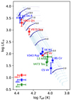 |
Fig. 1. Ten magnetic stars where rotational period variations have been detected shown on the HR diagram. Those showing a long-term increase in rotation period are represented in blue (decelerating), those with a decrease in green (accelerating), and those transitioning from an increase to a decrease (or vice versa) in red (oscillating). The solid curves represent the results of evolution calculations of nonrotating, nonmagnetic stars. Models with ZAMS masses from 1.5 to 5 M⊙ are shown at intervals of 0.1 M⊙, while models with ZAMS masses from 5.5 to 9.5 M⊙ are shown at intervals of 0.5 M⊙. The numbers displayed next to the solid curves represent the ZAMS mass. To indicate the ages, points were placed at ten equal divisions of the period from ZAMS to TAMS. |
We searched the literature for indications of these stars belonging to clusters or associations. σ Ori E is thought to belong to the σ Orionis Open Cluster (e.g., Tarricq et al. 2021), which is estimated to be 3–5 Myr old (Zapatero Osorio et al. 2002). V901 Ori is suggested to belong to the Ori B star-forming region, which has an age of 0.8–2.2 Myr (Román-Zúñiga et al. 2023), while V913 Sco may be part of Upper Sco with an age of 10–12 Myr (Esplin et al. 2018; Luhman & Esplin 2020). V343 Pup is also thought to belong to the Vela OB2 complex (Cantat-Gaudin et al. 2019). The age of this association is estimated to be 7.5–10 Myr from isochrones, which is somewhat inconsistent with the lithium depletion observed in pre-main-sequence stars (Prisinzano et al. 2016; Jeffries et al. 2017). While the estimated ages for the parent regions do not perfectly match our age estimates, no significant discrepancies are found due to the large uncertainties in our estimates. We did not find any studies that suggest relationships with known clusters and associations for the other stars in our sample.
2.2. Stellar models
The HOSHI code we used to compute stellar models is a general-purpose stellar evolution code designed to handle standard physics such as radiative and convective energy transfer, time-dependent chemical mixing, nuclear reactions, as well as stellar rotation and stellar magnetism. Here we briefly describe the most relevant elements of the code, the treatment of rotation and magnetic fields, and a more detailed description can be found in Takahashi & Langer (2021).
The code uses angular velocity as one of the independent variable to treat stellar rotation. As a critical assumption, our formulation treats that the angular velocity of the gas can be expressed as a function of the enclosed mass, Ω(M). This relies on the assumption known as the “shellular rotation law” (Zahn 1992), which adopts a picture where viscosity due to horizontal turbulence homogenizes the angular velocity on equipressure surfaces. The validity of this assumption will be discussed later.
The time evolution of the angular velocity distribution is determined by the following diffusion equation with an additional term that shows magnetic stress:
 (1)
(1)
where i, ρ, r, A, and B are the specific moment of inertia, density, radius, toroidal vector potential expressing poloidal magnetic component, and toroidal magnetic component, respectively, all of which are functions of mass. νcv is the viscosity due to convective turbulence and is estimated as νcv = υcvlcv/3 using the convective velocity υcv and length scale lcv provided by the mixing-length theory. A fudge factor ncv is introduced to absorb our ignorance of angular momentum transport due to convective turbulence. In this work, ncv = 0 is used so that convective regions rotate rigidly. νeff is the effective viscosity due to turbulence caused by instabilities other than convection. The dynamical and secular shear instability, the Solberg-Hoiland instability, and the Goldreich-Schubert-Fricke instability are included here as instabilities due to rotation (Pinsonneault et al. 1989; Heger et al. 2000), and the Pitts-Tayler instability as instability due to magnetic fields (Spruit 2002; Maeder & Meynet 2004). The boundary condition is to set all angular momentum fluxes to zero at the inner and outer boundaries.
The evolution of the stellar magnetic field is represented by the time evolution of two functions, A(M) for the poloidal component and B(M) for the toroidal component:
 (2)
(2)
 (3)
(3)
η represents the effective magnetic viscosity. It is estimated as η = νcv + fm × νeff with a parameter fm. The control parameter fm is introduced to handle the large uncertainty of the turbulent transport coefficients, but fm = 1 is used in this study. The inner boundary conditions are chosen as ∂(A/r)/∂M = 0 and ∂(B/r2)/∂M = 0 so that the magnetic fields do not diverge and are smoothly connected to the solution of the diffusion equations at the center. At the stellar surface, we assumed that the poloidal component smoothly connects to the external dipole field, and the toroidal component was set to zero because the electric current is assumed not to penetrate the stellar surface. These are expressed by ∂(Ar2)/∂M = 0 and B = 0.
2.3. The eigenmode analysis
We adopted the working hypothesis that the observed variations in the rotational period represent standing torsional Alfvén waves. For the analysis of the torsional Alfvén waves, we utilized Eqs. (1) and (3). This is because numerical experiments that used the HOSHI code have shown that these equations can describe not only the propagation of torsional Alfvén waves but also their standing waves (Takahashi & Langer 2021).
Standing waves can be expressed as eigenmodes of a certain differential operator. Therefore, we conducted an eigenmode analysis to find standing-wave solutions instead of directly solving the wave propagation and scanning the frequency space as done in Krtička et al. (2017). With this method, each eigenmode, including higher-order modes can be efficiently and robustly obtained.
The assumptions applied for the formulation are twofold. First, we assumed that physical quantities other than Ω and B, such as the radius, the density, and the poloidal component of the magnetic field, remain constant over time. This assumption is justified by the fact that the oscillation periods of the standing waves derived from the analysis are much shorter than the evolutionary timescales of quantities like radius. Additionally, we limited our scope to standing waves that can be expressed as linear responses to the equilibrium state. While nonlinear standing waves influenced by higher-order terms may exist, we did not explore such cases in this study.
For the formulation, we first discretized the differential equation and then linearized it to obtain the eigenmode equation. The discretized form of the evolution equations (Eqs. (1) and (3)) are schematically expressed as
 (4)
(4)
where X = (Ω, B) is a set of the two unknown variables and F expresses a discretized differential operator that includes spatial partial derivatives acting on X. In the numerical computation, X is expressed as a finite-component vector, and F is treated as a nonlinear function of X.
Next, to investigate the linear response to the equilibrium state, the independent variable X is separated as X = X0 + δX and the schematic evolution equation is expanded around X0 up to the first order of δX as
 (5)
(5)
where X0 is a time-constant vector corresponding to the equilibrium state so that F(X0) = 0, δX is the perturbation, and F′=∂F/∂X is the Jacobian of F(X).
Since we are interested in solutions that behave as standing waves, we focused on δX, which is separable into temporal and spatial components. Furthermore, we assumed that the time dependence takes an exponential form, δX = Θ(M)exp(λt). This allowed us to define an eigenvalue problem for the Jacobian F′ as
 (6)
(6)
which is the main equation we treat in this work.
The eigenvalue λ can be decomposed into the real part (σ) and the imaginary part (ω),

where i in this equation shows the imaginary unit, and a nonzero imaginary part means that the eigenmode shows an oscillatory evolution. Because we interpreted this oscillatory evolution as the rotational period variation observed in some magnetic stars, the period of the variation, Π, can be estimated as Π = 2π/ω using the eigenvalue in this model. We investigate the properties of Π later on. One of the limitation of this model is that, since it is based on a linear analysis, it cannot predict the amplitude of the rotational period variation; this requires some kind of driving mechanism, which is beyond the scope of the present study.
In practice, F′ can be evaluated by reusing the Jacobian employed in the main Newton-Raphson iteration for evolution simulations. Hence, our eigenmode analysis shares the spacial resolution with the stellar evolution simulation. The mesh number is typically ∼1000. The eigenmode analysis of the F′ matrix is done using the DGEEV subroutine in the open library LAPACK.
Equation (4) is the discretized representation of the differential Eqs. (1) and (3) and is identical to the equations handled in the stellar evolution simulation with the HOSHI code. The equation includes nonlinear viscosity and diffusion terms, and Eq. (5) is obtained by linearizing them. However, because the expected oscillations were obtained by the time evolution simulations when the eigenmodes derived from the linearized equation were used as initial conditions for Eq. (4), the nonlinear effects are considered to be minor. We also note that, aside from the inclusion of the linearized dissipation terms, Eq. (5) is essentially the same as the linear wave equation analyzed in Takahashi & Langer (2021).
2.3.1. The parametric structure of the poloidal magnetic field
The magnetic field structure of stellar interiors remains a perplexing subject. In this study, the strategy is to describe the internal structure of the poloidal magnetic field using a simple parametric function with minimal assumptions. First, the magnetic field is assumed to be axisymmetric to the axis of rotation, as in the basic definition of our evolution simulation. Second, the radial dependence is expressed using the parameter nBrad as
 (7)
(7)
where Rcv and Rstar are the radius of the central convective region and the stellar radius and Bpole is the magnetic flux density at the pole on the stellar surface. The magnetic stars considered in this work are early-type main-sequence stars, and all of them have a convective region in the center. Therefore, the magnetic field does not diverge or go to zero at the center using this expression. Then, the radial field is converted into the A function as A = Brad × r/2. Figure 2 shows magnetic field structures with different nBrad applied to the CU Vir model as an example.
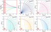 |
Fig. 2. Examples of the parametric poloidal field structures applied in this work. Solid lines in the top-left panel show the radial dependences of Brad/Bpole(r) functions with nBrad = −2.0 (dark blue), −1.0 (magenta), +0.0 (green), +1.0 (yellow), and +2.0 (cyan). The red-hatched region in the stellar center corresponds to the central convective region, in which the magnetic field is assumed to be constant. The vertical solid red line indicates the stellar surface, where Brad/Bpole(r) = 1. The remaining plots show the two-dimensional poloidal field structures in the meridional cuts. As in the top-left panel, the red-hatched area shows the central convective region and the solid red curve is the stellar surface. |
2.3.2. Characteristics of Π
As noted in Krtička et al. (2017), the eigenvalue λ follows a scaling transformation of λ′=γ−1λ with Bpole′=γBpole due to the linear dependence of the matrix F on Bpole. Hence, a linear relationship between Π and Bpole can be obtained:
 (8)
(8)
One can calculate the Π for models with different values of Bpole using this relationship. Furthermore, the uncertainty in Bpole is associated with the uncertainty in Π through this relationship.
Another interesting characteristic of Π is that it is largely independent of the background rotational distribution, Ω(M). At the formulation level, this arises because the Jacobian F′ depends only weakly on Ω due to the small Ω-dependence of the diffusivity and viscosity. In contrast, an alternative hypothesis for explaining rotational variation, precession, predicts a period of a rotational variation that is proportional to the rotation period (Shore & Adelman 1976). If the dependence can be derived from a large sample of variability observation, it will provide constraints on the model.
3. Results
3.1. General trends of the eigenmode analysis
First, we discuss the general trends of the eigenmode analysis by taking the CU Vir model as an example. The background structure is taken from a model with Mini= 3.0 M⊙ and τ= 54.5 Myr. In Fig. 3, lowest-order eigenmodes from the first to the fourth obtained for the model with nBrad = +1.0 are shown as a function of radius. In the central convective region, Ω profiles become flat and B(r) profiles become ∝r2 due to the large diffusion coefficient. Outside the convective region, both profiles show characteristic oscillatory patterns, whose number of nodes corresponds to the order. For example, for the lowest-order mode, the number of nodes in the Ω and B profiles are 1 and 0, respectively, and it increases by one as the order of the eigenmode increases. And the frequency of the torsional oscillation, Π = 2π/ω, decreases as the order of the mode increases.
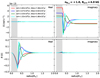 |
Fig. 3. Eigenfunctions obtained for the CU Vir model with nBrad = +1.0. Top panels: Distribution of angular velocity, Ω(r). Bottom panels: Toroidal magnetic field component, B(r). In each row, the left panel shows the real part, and the right panel the imaginary part. The modes from the lowest to the fourth are indicated as red, blue, green, and cyan lines. The reciprocals of the eigenvalues for each mode are shown in the legend. The gray-shaded area indicates the central convective region. |
The nBrad dependence of the period of torsional oscillation is shown in Fig. 4. With the observational constraint of Bpole = 4.0 kG for CU Vir (Kochukhov et al. 2014; Shultz et al. 2022), nBrad becomes the only parameter left to specify the internal poloidal field structure in our formulation. The figure shows that the larger the value of nBrad, the longer the oscillation periods irrespective to the order. Hence, there is a simple one-to-one relationship between the parameter nBrad and the frequency of oscillations. This relationship indicates that, within a crude approximation of the internal B-field structure, the structure of the internal poloidal field can be inferred by observing the period of torsional oscillations. Specifically, there are long enough observations for CU Vir, indicating that the rotation period may oscillate with a period Π = 67.6 yr. This period can be explained as the fundamental mode of the torsional oscillation with nBrad ∼ +1.0, indicating that the internal B-field is slightly concentrated on the stellar surface, rather than the center, for this particular case.
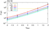 |
Fig. 4. Dependence of oscillation periods on nBrad estimated for the CU Vir model for eigenfunctions from the first to the fourth orders. Different line styles are used for first (red, circle), second (blue, square), third (green, triangle), and fourth (cyan, cross). For comparison, tcross is indicated by a dotted black line. The constant value (dashed yellow line) corresponds to the oscillation period suggested for CU Vir (67.6 yr). |
The figure also shows that the frequency of the lowest order agrees well with the crossing time of the torsional Alfvén wave. The crossing time is estimated as
 (9)
(9)
where  is the characteristic speed of the torsional Alfvén wave in our formulation (Takahashi & Langer 2021). This equation indicates that the region with the slowest wave propagation speed dominates the overall crossing time. Additionally, the strength of the poloidal magnetic field is proportional to the wave propagation speed and inversely proportional to the crossing time. This gives a physical explanation of the relation Eq. (8).
3.2. Variation periods with different background structures
The variation period Π depends not only on the magnetic field structure but also on the background density structure. Figure 5 illustrates how Π varies as the mass and age of the background structure model are changed while keeping the parameters specifying the magnetic field structure. It not only shows that Π depends on the background model, but also demonstrates how this dependence varies with nBrad. Namely, for the case where the magnetic field is concentrated on the surface (nBrad = +1.0), Π increases with increasing age and decreasing mass. Conversely, for the case where the magnetic field is centrally concentrated (nBrad = +1.0), the trend reverses, and Π increases with decreasing age and increasing mass. However, the change in Π due to differences in the background structure remains at most a factor of a few, which is relatively small compared to the change due to differences in nBrad, which can span several orders of magnitude.
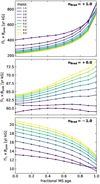 |
Fig. 5. Variation periods, Π, for different background structures with different fractional main-sequence ages and masses. The three panels show results with nBrad of +1.0 (top), +0.0 (middle), and −1.0 (bottom). The dependence on Bpole is implicitly included in the y-axis based on the relation Eq. (8). |
Different values of nBrad lead to varying dependences on the background, and most importantly, changing the value of Π significantly. This characteristic should be closely related to the velocity distribution of torsional Alfvén waves within the star, in particular, the distribution of propagation time in bottleneck regions. To explore this, the distribution of inverse of the Alfvén velocity is plotted in Fig. 6 for Mini = 3 M⊙ models with different ages. The top panel illustrates the results for nBrad = +1.0, while the middle and bottom panels are for nBrad = +0.0 and −1.0, respectively. In this figure, the area enclosed by the lines and the x-axis corresponds to the crossing time.
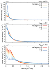 |
Fig. 6. Inverse of the velocity of the torsional Alfvén wave as a function of radius. The enclosed area by the curves corresponds to the crossing time. From top to bottom, results for nBrad = +1.0, +0.0, and −1.0, with Bpole = 1 kG are shown. The density distributions are based on the 3 M⊙ model. Each panel includes 11 lines corresponding to different fractional main-sequence ages of 0.0, 0.1, …, 1.0, with the color of the lines changing from red to blue. Filled circles represent a change in radius. |
The figure shows that the region where Alfvén waves slow down the most is the central part of the star, regardless of the magnetic field structure. This indicates that, even with nBrad = −1.0, the increase in density at the center is responsible for determining the speed of Alfvén waves. On the other hand, despite keeping the surface magnetic field strength constant, the speed of Alfvén waves changes by an order of magnitude with different nBrad. This is why the crossing time and Π show the large nBrad dependence.
In the case of nBrad = +0.0, the wave velocity distribution remains relatively unchanged as the star ages. In this model, a uniform magnetic field of constant strength is imposed throughout the stellar interior, and the wave velocity is only affected by variations in the density distribution. Therefore, the time-constant nature indicates that changes in the density distribution during main-sequence star evolution itself do not have a significant impact on the oscillation period evolution. On the other hand, for nBrad = ±1.0, the changes in density distribution have a stronger impact on the variation period. This is because, when using our magnetic field structure description, the field strength in the central region directly depends on the stellar radius. The larger the age of the model, the larger the radius. Hence, in the case of nBrad = +1.0, the central magnetic field becomes weaker, causing the velocity to slow down. Conversely, for nBrad = −1.0, the central field becomes stronger, resulting in faster wave velocities. In other words, the change in the variation period with different ages can be attributed to the simplification of the magnetic field structure used in this work rather than being a direct physical consequence of stellar evolution.
3.3. Eigenmode analysis for specific magnetic stars
The same analysis as conducted on CU Vir is applied to the other nine magnetic stars that are listed in Table 1, and the results are shown in Fig. 7 for all ten stars. To perform eigenmode analysis using our model, it is necessary to set the magnetic field strength on the stellar surface. As noted in Sect. 2, we could not find such values for V343 Pup, 13 And, V473 Tau, and BS Cir, so a typical value of Bpole = 1 kG is applied for these stars. The obtained periods follow the relationship Π × Bpole = const. Consequently, they may linearly shift upward and downward based on the actual field strength.
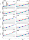 |
Fig. 7. Same as Fig. 4 but for all the magnetic stars where rotational period variations have been observed. |
Detecting rotational period variations requires long-term monitoring, and for each star, the duration of this extended monitoring is indicated as Tbaseline. It is expected that modes with periods shorter than Tbaseline have already been detected through previous monitoring. However, this contradicts the fact that there have been no cases where the periodicity of rotational period variations has been definitively confirmed, even for CU Vir. Consequently, magnetic field structures that have such modes can be rejected. On the other hand, field structures with longer periods than Tbaseline are allowed observationally. In the figure, this condition is represented with a gray or white background. Based on this condition, it is concluded that centrally concentrated magnetic field structures with a negative nBrad is rejected for all magnetic stars.
Although not yet settled, changes in the sign of rotational period variations have been detected for V901 Ori, V913 Sco, and CU Vir, and these changes enable the estimation of the variation periods (dashed yellow lines). Our theoretical model predicts that the variation period has a strong dependence on nBrad. Therefore, the model can place strong constraints on the corresponding range of nBrad when the period is given, and the periods for these stars can be explained by setting nBrad ≳ 1.0. This might suggest that the magnetic field structure inside the stars is strong near the surface.
4. Discussion
4.1. Limitations of our model
In our framework, a key assumption for one-dimensionalization is the shellular rotation law, where the material at the same radius (originally on an isopressure surface) is assumed to have the same angular velocity. This assumption is justified if structural changes occur on the timescale of stellar evolution since it is sufficiently long to allow turbulent viscosity originating from horizontal turbulence to relax the angular momentum distribution. However, it is uncertain whether the same process occurs on the Alfvén timescale, which is much shorter than the evolutionary timescale. Instead, one might consider that differential rotation develops in the horizontal direction during the propagation of Alfvén waves.
Without assuming shellular rotation, Alfvén waves traveling along different magnetic field lines would have distinct crossing times. In this case, differential rotation between gas associated with adjacent magnetic field lines can induce turbulence, causing phase mixing (cf., Charbonneau & MacGregor 1992, 1993). To determine oscillation periods of stationary Alfvén waves in this context, a two-dimensional linear analysis, considering the efficiency of phase mixing, will be suitable.
Taking this into account, in the current one-dimensional framework, the model’s accuracy is expected to decrease as the crossing time for each magnetic field line becomes different. Figure 2 suggests that in centrally concentrated magnetic field structures (nBrad ≲ 0), where path lengths are close, the model’s accuracy might not be severely affected. Conversely, in surface-concentrated magnetic field structures (nBrad ≳ 0), there could be a potential mismatch between the predictions of our one-dimensional model and future two-dimensional models.
Another influential simplification is our assumption that the rotation and the magnetic axes are aligned. In reality, it is common for the two axes not to align, so that analyses using the oblique rotator model are commonly conducted. However, our analysis has also shown that the period of rotational period variations is simply determined by the Alfvén wave crossing time. Therefore, even when considering the obliquity, we expect only a few-fold difference in the variation periods, which is unlikely to affect the conclusions of this study.
In upper main-sequence stars, a strong dynamo-generated magnetic field can exist within the convective core (e.g., Featherstone et al. 2009; Augustson et al. 2016). The polarity of dynamo-driven fields can reverse. It is thus reasonable to assume that the dynamo-generated field is not directly connected to the stable magnetic field in the radiative layer. In a one-dimensional model, this disconnection can be represented by setting the magnetic field strength to zero at the boundary of the convective region. However, in our approach, the zero magnetic field causes the local crossing time to diverge, making it complicated to estimate the crossing time. Due to this issue, applying our model to cases with strong dynamo fields remains challenging. However, the radius of the convective core region is relatively small, and its crossing time is not expected to dominate over the crossing time of the outer radiative layers. Therefore, our current analysis is expected to provide a reasonable order of magnitude estimate of the oscillation period.
4.2. Comparison with Krticka’s model
Krtička et al. (2017) also analyzed the rotational period variations of CU Vir and V901 Ori based on the picture that the variations are induced by standing Alfvén waves. The one-dimensional magnetohydrodynamic (MHD) equations they obtained are similar to ours, but they use a different poloidal magnetic field configuration, which is expressed in the (R, Z) plane as
 (10)
(10)
where B is a constant. Their model yielded oscillation periods of 51 years for CU Vir and 5 years for V901 Ori. As a result, they concluded that the rotational period variation observed in CU Vir, with a period of approximately 70 years, can be explained by standing Alfvén waves. However, the variation in V901 Ori, estimated to have a period of over 100 years, cannot.
While dealing with similar models, our work has resulted in different conclusions. The main factor contributing to this difference is likely to be the different assumptions about the poloidal magnetic field structure. As demonstrated earlier, our model can alter the period of standing Alfvén waves by several orders of magnitude by changing the radial dependence of the poloidal magnetic field. On the other hand, it can be inferred that Krticka’s model, which has only tested a single field structure, had a limited range of explainable periods. Regarding the surface magnetic field, Krticka applied Bp = 10 kG, given the highly complex surface magnetic field structure. In contrast, we employed a dipole component of 6.1 kG obtained from Shultz et al. (2019b). While using a weaker value results in longer oscillation periods, the effect is considered minor, at most doubling the period.
4.3. Estimating the magnetic field structure based on the rotational period variation
Centrally concentrated magnetic fields appear unlikely based on the lack of detected oscillations in most stars. If they were, Alfvén waves would rather quickly pass through the entire star, resulting in a sufficiently short period of the rotational period variation to be detected. Comparison with three stars that potentially show cyclic variations (V901 Ori, CU Vir, and V913 Sco) suggests that the degree of surface concentration of the internal poloidal field is moderate (nBrad ∼ +1).
The geometry of magnetic fields in equilibrium in the stellar interior has been investigated with MHD simulations (e.g., Braithwaite & Spruit 2004; Becerra et al. 2022) and analytical approaches (e.g., Lyutikov 2010; Duez & Mathis 2010; Akgün et al. 2013). The surface-concentrated magnetic field structures as described in our model (nBrad > 0) resemble the equilibrium structures obtained numerically (Braithwaite & Spruit 2004) more than the central-concentrated structure (nBrad < 0).
If the estimates of surface concentration for the three stars that show cyclic variations were quantitatively accurate, the most massive of them, V901 Ori, exhibits the strongest surface concentration (nBrad ∼ +1.7), suggesting that the degree of surface concentration correlates with the mass of the stars. Another possibility is that, considering that the age of V901 Ori is almost zero while the fractional main-sequence ages of V913 Sco and CU Vir are in the range of 0.1–0.3, the initially more surface-concentrated magnetic field would permeate deeper into the star as it evolves. There are indications that the magnetic field structure of magnetic stars becomes simplified with age (Rusomarov et al. 2015; Silvester et al. 2015). It is also possible that such a global evolution is occurring simultaneously within the stellar interior. However, this evolutionary scenario contradicts the results of Braithwaite & Nordlund (2006), where the poloidal field stabilized by the toroidal field rises to the surface due to magnetic diffusion over time, weakening the magnetic field strength near the center.
Our analysis is limited by the small sample size and the simple quantification methods. Additionally, V901 Ori is known to have a highly complex surface magnetic field structure (Kochukhov et al. 2010), unlike the largely dipolar magnetic fields of CU Vir (Kochukhov et al. 2014) and V913 Sco (Shultz et al. 2019a). Further research is necessary to validate trends and dependences related to the internal magnetic field.
4.4. Implications of strong magnetic fields detected in red giant stars
Li et al. (2023) reported that the shift in dipole mode frequency observed in red giants can be explained by a strong magnetic field of 20–150 kG above the H-burning shell. In this subsection we compare the constraints derived from asteroseismology with our proposed scenario.
First, based on the results of an evolutionary calculation of a (non-magnetic) 1.5 M⊙ star, the required magnetic field strength at the terminal age main sequence (TAMS) to reproduce the observed constraints in the H-burning shell of red giant stars are estimated. Here, we assumed that the magnetic field in the H-burning shell is a remnant of the field present at TAMS, because this region belongs to the radiative zone during the main-sequence evolution and is thus unlikely to be affected by dynamo processes. A more detailed stellar evolution calculation incorporating magnetic fields will be conducted in future works.
Under this assumption, the magnetic field strength evolves according to magnetic flux conservation. The H-burning shell of a red-giant star had a larger radius when the star was on the main sequence. From our model, the radius ratio is estimated to be

where rMS and rRG are the radius of the region at a mass coordinate of 0.19–0.21 M⊙, which corresponds to the H-burning shell, during the main-sequence and red-giant phases, respectively. Since the magnetic flux, the conserved quantity, is proportional to Br2, where B represents the magnetic field strength, the ratio of the magnetic field strength between the two phases becomes
Applying this factor to the constraints from asteroseismology, the red giant stars in Li’s sample are estimated to have magnetic fields of approximately 1–10 kG in the radiative region around 0.2 M⊙ during their main-sequence phase. Most of the stars in Li’s sample were likely normal non-magnetic stars during their main-sequence phase, so their surface magnetic field was at most on the order of ∼1 G. This means that the red giants analyzed by Li et al. had a centrally concentrated magnetic field during their main-sequence phase, which contradicts our conclusions.
Similarly, by applying the same factor to our main-sequence model, we can estimate the strength of the poloidal field in the H-burning shell of red giant stars. Since the radius of the H-burning shell precursor at TAMS is approximately 1/20 of the stellar radius, using the parameters that explain CU Vir, nBrad = +1, and a surface magnetic field of 1 G, the radiative region at ∼0.2 M⊙ is estimated to have a poloidal field of 0.05 G at TAMS. If this magnetic field is enhanced by a factor of 16 due to contraction, the poloidal field strength in the H-burning shell of the red giant is estimated to be around 1 G, which is five orders of magnitude smaller than the estimate by Li et al. This discrepancy suggests that the red giant stars in which magnetically induced oscillation frequency shifts have been detected were strong magnetic stars on their main-sequence phase, possessing surface fields exceeding 100 kG.
Li et al. provided an alternative interpretation for the origin of the frequency shift: The kernel function used to estimate the frequency shift is also sensitive to the region inside the H-burning shell. The observed frequency shift can then be explained by a magnetic field of 200–300 kG in the former convective core region, which can be accounted for by a convective dynamo driven by hydrogen burning. Our results are more consistent with this alternative interpretation. Hence, this lead to the conclusion that a convective dynamo operates during hydrogen burning, and the magnetic field it generates remains after the cease of the core convection and causes the frequency shift observed in red giants. It should be noted that the method we used in this study is agnostic regarding the magnetic field distribution inside the stellar convective core. Thus, we do not rule out the possibility that a strong magnetic field, which is likely disconnected from the radiative layer, exists within the convective core.
Main-sequence stars with masses of less than around 1 M⊙ are considered to form radiative cores (Kippenhahn & Weigert 1990). Even in such low-mass stars, it is predicted that a small convective core forms due to non-equilibrium hydrogen burning mediated by 3He and 12C occurring just before the star enters the ZAMS. However, it is uncertain whether such a short-lived convective core can efficiently drive a dynamo, and if it can, whether the magnetic field will survive without dissipating during the long main-sequence phase that follows. Hence, it is less likely that low-mass red giants possess strong internal magnetic fields similar to those of higher-mass red giants.
Therefore, the most direct way to determine the origin of the frequency shift will be to investigate whether similar shifts are seen in the low-mass red giants. Considering the inverse correlation between age and mass, finding and analyzing low-mass red giants may be less feasible, and the least massive star in the sample by Li et al. is estimated to have a mass of about 1.04 solar masses. Nevertheless, the Kepler targets include a non-negligible number of low-mass red giants (e.g., Yu et al. 2018). Investigating older, less massive red giants could shed light on this question.
4.5. Excitation mechanisms of standing Alfvén waves in magnetic AB stars
Magneto-sonic oscillations are thought to exist in magnetars, as signified by the quasi-periodic oscillations in the tail of giant X-ray flares (e.g., Strohmayer & Watts 2005), as the oscillation frequency is well reproduced by global MHD simulations (Glampedakis et al. 2006; Gabler et al. 2018). In this case, fractures in the crust of the magnetar are thought to disturb the hydrostatic equilibrium, which can provide the excitation of the MHD waves.
It is not known what could excite Alfvén waves in magnetic main-sequence stars. Since the ages of the investigated magnetic stars span several to a few hundred megayears, which corresponds to 105…107 oscillation periods, it appears unlikely that an event relating to the formation of these stars excited oscillations that are still ongoing. On the other hand, the nuclear evolution of the considered main-sequence stars imposes changes in the rotation period on the order of 10−10 s s−1, which is comparable to the observed period variations of 10−2 s yr−1 ∼ 3 × 10⁻¹⁰ s s−1. Given these rough estimates, it appears possible that the observed period changes are produced by standing Alfvén waves driven by changes in the internal shear layers on the nuclear timescale.
Furthermore, coupling between the core convection and the envelope magnetic field could excite magneto-sonic waves. Indeed, for red giant stars, Lecoanet et al. (2017) found that internal gravity waves can be efficiently converted into magnetic waves under certain conditions. Finally, Krtička et al. (2017) suggested that coupling of a stellar wind with the stellar magnetosphere could excite Alfvén waves. While sufficiently strong winds are not predicted for late B and A type stars, their presence is suggested for CU Vir based on its periodic radio emission (Trigilio et al. 2000).
4.6. Toward future detections of rotational period variations
If we assume that the typical surface concentration of the magnetic field resembles our case nBrad ∼ +1, the period of cyclic variations is expected to inversely correlate with the strength of the surface magnetic field (Eq. (8)) and to show an increasing correlation with age and a decreasing correlation with mass (Fig. 5). Based on these trends, it would be possible to devise strategies to discover new stars exhibiting rotational period variations, and even more, cyclic variations.
Among the ten magnetic stars analyzed in this study, most of those with known surface field strength have observational baselines comparable to the predicted periods for the case nBrad = +1. Within the next few decades, it may be possible that the second time derivative of the rotation period will be measured in these stars. 56 Ari has an exceptionally short observational baseline compared to the nBrad = +1 period, which suggests that the rotational period variations of this star are not due to the Alfvén wave but rather due to precession (Shore & Adelman 1976; Adelman & Fried 1991). Determinations of the rotational period for this star have not been reported since 2001 to our knowledge. The passage of more than 20 years will aid in the detection of the second derivative component of rotational period variations, which is essential for constraining models.
For stars without constraints on surface magnetic fields, we estimate the nBrad = +1 periods for a typical field strength of 1 kG, and their values are generally one order of magnitude larger than observational baselines. The difference in timescales suggests that these stars have relatively strong surface magnetic fields, around 10 kG. Alternatively, they could possess relatively centrally concentrated internal magnetic fields (nBrad ∼ +0). If the surface magnetic fields of these stars were weaker, around 100 G, it might contradict the idea that rotational period variations are due to Alfvén waves, suggesting instead that they are caused by precession. Hence, when magnetic stars exhibiting variations of the rotational period are discovered, it is crucial to estimate the surface magnetic field strength through spectropolarimetric observations.
Until now, the detection of rotational period variations has been biased toward rapidly rotating stars with rotation periods of around one day. This is because a shorter rotation period makes it easier to meet the condition of observing as many cycles of rotation as possible, which is required for detecting rotational period variations (Pyper & Adelman 2020). However, such rapidly rotating magnetic stars are biased toward younger stars (Fossati et al. 2016; Shultz et al. 2018; Keszthelyi et al. 2020), and it is known that the majority of magnetic stars have longer rotation periods, peaking around three days (Kochukhov & Bagnulo 2006; Netopil et al. 2017). It is important to search for rotational period variations in the more common magnetic stars with longer rotation periods and relatively old ages.
Another factor, the amplitude, is preferable to be large for the detection of rotational period variation. In this study, linear analysis is conducted so that the investigation of the amplitude is not feasible. To do so, further research is needed on how the rotational period variation is driven and to what extent the long-term growth and dissipation occur.
5. Concluding remarks
We have explored the existence and properties of torsional Alfvén waves in magnetic stars on the upper main sequence. Based on the concepts developed in Takahashi & Langer (2021), we performed an eigenmode analysis of standing Alfvén waves in such stars and derived the most likely oscillation frequencies. We did this while assuming different degrees of the central or surface concentration of the magnetic field, which results in largely different frequencies.
We compared our results with the rate of change of the stellar rotation period and find, as Krtička et al. (2017), that they can be compatible with the periods of the standing Alfvén waves. Our results imply compatibility only for the case in which the magnetic fields in these stars are concentrated toward the stellar surface; however, they show the potential of this type of technique for exploring the properties of the magnetic field in stellar envelopes.
Acknowledgments
K.T. thanks to Kengo Tomida and Fabian Schneider for fruitful discussions. This work was supported in part by JSPS KAKENHI Grant Numbers JP22K20377, JP24K17102.
References
- Adelman, S. J., & Fried, R. E. 1991, Int. Amateur-Professional Photoelectric Photometry Commun., 45, 4 [NASA ADS] [Google Scholar]
- Adelman, S. J., Dukes, R. J. Jr., & Pyper, D. M. 1992, AJ, 104, 314 [NASA ADS] [CrossRef] [Google Scholar]
- Adelman, S. J., Malanushenko, V., Ryabchikova, T. A., & Savanov, I. 2001, A&A, 375, 982 [NASA ADS] [CrossRef] [EDP Sciences] [Google Scholar]
- Akgün, T., Reisenegger, A., Mastrano, A., & Marchant, P. 2013, MNRAS, 433, 2445 [Google Scholar]
- Augustson, K. C., Brun, A. S., & Toomre, J. 2016, ApJ, 829, 92 [Google Scholar]
- Babcock, H. W. 1947a, ApJ, 105, 105 [NASA ADS] [CrossRef] [Google Scholar]
- Babcock, H. W. 1947b, PASP, 59, 260 [Google Scholar]
- Babcock, H. W. 1948, PASP, 60, 245 [Google Scholar]
- Babcock, H. W. 1949, Observatory, 69, 191 [Google Scholar]
- Babcock, H. W. 1958, ApJS, 3, 141 [Google Scholar]
- Becerra, L., Reisenegger, A., Valdivia, J. A., & Gusakov, M. 2022, MNRAS, 517, 560 [NASA ADS] [CrossRef] [Google Scholar]
- Beck, P. G., De Ridder, J., Aerts, C., et al. 2012, Astron. Nachr., 333, 967 [NASA ADS] [CrossRef] [Google Scholar]
- Belopolsky, A. 1913, Astron. Nachr., 196, 1 [CrossRef] [Google Scholar]
- Braithwaite, J., & Nordlund, Å. 2006, A&A, 450, 1077 [NASA ADS] [CrossRef] [EDP Sciences] [Google Scholar]
- Braithwaite, J., & Spruit, H. C. 2004, Nature, 431, 819 [Google Scholar]
- Braithwaite, J., & Spruit, H. C. 2017, R. Soc. Open Sci., 4, 160271 [Google Scholar]
- Cantat-Gaudin, T., Mapelli, M., Balaguer-Núñez, L., et al. 2019, A&A, 621, A115 [NASA ADS] [CrossRef] [EDP Sciences] [Google Scholar]
- Charbonneau, P., & MacGregor, K. B. 1992, ApJ, 387, 639 [NASA ADS] [CrossRef] [Google Scholar]
- Charbonneau, P., & MacGregor, K. B. 1993, ApJ, 417, 762 [Google Scholar]
- Cox, A. N. 2000, Allen’s Astrophysical Quantities (New York: Springer) [Google Scholar]
- Deheuvels, S., Doğan, G., Goupil, M. J., et al. 2014, A&A, 564, A27 [NASA ADS] [CrossRef] [EDP Sciences] [Google Scholar]
- Deheuvels, S., Li, G., Ballot, J., & Lignières, F. 2023, A&A, 670, L16 [NASA ADS] [CrossRef] [EDP Sciences] [Google Scholar]
- Deutsch, A. J. 1947, ApJ, 105, 283 [Google Scholar]
- Deutsch, A. J. 1954, Trans. Int. Astron. Union, 8, 801 [Google Scholar]
- Deutsch, A. J. 1958, in Electromagnetic Phenomena in Cosmical Physics, ed. B. Lehnert, 6, 209 [NASA ADS] [Google Scholar]
- Duez, V., & Mathis, S. 2010, A&A, 517, A58 [NASA ADS] [CrossRef] [EDP Sciences] [Google Scholar]
- Esplin, T. L., Luhman, K. L., Miller, E. B., & Mamajek, E. E. 2018, AJ, 156, 75 [NASA ADS] [CrossRef] [Google Scholar]
- Featherstone, N. A., Browning, M. K., Brun, A. S., & Toomre, J. 2009, ApJ, 705, 1000 [Google Scholar]
- Feiden, G. A., & Chaboyer, B. 2012, ApJ, 761, 30 [NASA ADS] [CrossRef] [Google Scholar]
- Feiden, G. A., & Chaboyer, B. 2013, ApJ, 779, 183 [Google Scholar]
- Feiden, G. A., & Chaboyer, B. 2014, ApJ, 789, 53 [NASA ADS] [CrossRef] [Google Scholar]
- Ferrario, L., & Wickramasinghe, D. 2006, MNRAS, 367, 1323 [NASA ADS] [CrossRef] [Google Scholar]
- Fossati, L., Schneider, F. R. N., Castro, N., et al. 2016, A&A, 592, A84 [NASA ADS] [CrossRef] [EDP Sciences] [Google Scholar]
- Fuller, J., Cantiello, M., Stello, D., Garcia, R. A., & Bildsten, L. 2015, Science, 350, 423 [Google Scholar]
- Fuller, J., Piro, A. L., & Jermyn, A. S. 2019, MNRAS, 485, 3661 [NASA ADS] [Google Scholar]
- Gabler, M., Cerdá-Durán, P., Stergioulas, N., Font, J. A., & Müller, E. 2018, MNRAS, 476, 4199 [NASA ADS] [CrossRef] [Google Scholar]
- Georgy, C., Meynet, G., Ekström, S., et al. 2017, A&A, 599, L5 [NASA ADS] [CrossRef] [EDP Sciences] [Google Scholar]
- Glampedakis, K., Samuelsson, L., & Andersson, N. 2006, MNRAS, 371, L74 [CrossRef] [Google Scholar]
- Griffiths, A., Eggenberger, P., Meynet, G., Moyano, F., & Aloy, M.-Á. 2022, A&A, 665, A147 [NASA ADS] [CrossRef] [EDP Sciences] [Google Scholar]
- Guthnick, P., & Prager, R. 1914, Photoelektrische Untersuchungen an Spektroskopischen Doppelsternen und an Planeten (Berlin: Ferd. Dümmlers Verlagsbuchhandlung) [Google Scholar]
- Hatt, E. J., Ong, J. M. J., Nielsen, M. B., et al. 2024, MNRAS, 534, 1060 [NASA ADS] [CrossRef] [Google Scholar]
- Heger, A., Langer, N., & Woosley, S. E. 2000, ApJ, 528, 368 [NASA ADS] [CrossRef] [Google Scholar]
- Heger, A., Woosley, S. E., & Spruit, H. C. 2005, ApJ, 626, 350 [Google Scholar]
- Jeffries, R. D., Jackson, R. J., Franciosini, E., et al. 2017, MNRAS, 464, 1456 [Google Scholar]
- Keszthelyi, Z. 2023, Galaxies, 11, 40 [NASA ADS] [CrossRef] [Google Scholar]
- Keszthelyi, Z., Meynet, G., Georgy, C., et al. 2019, MNRAS, 485, 5843 [NASA ADS] [CrossRef] [Google Scholar]
- Keszthelyi, Z., Meynet, G., Shultz, M. E., et al. 2020, MNRAS, 493, 518 [NASA ADS] [CrossRef] [Google Scholar]
- Kippenhahn, R., & Weigert, A. 1990, Stellar Structure and Evolution (New York, Berlin, Heidelberg: Springer-Verlag) [Google Scholar]
- Kochukhov, O., & Bagnulo, S. 2006, A&A, 450, 763 [NASA ADS] [CrossRef] [EDP Sciences] [Google Scholar]
- Kochukhov, O., Lundin, A., Romanyuk, I., & Kudryavtsev, D. 2010, ApJ, 726, 24 [Google Scholar]
- Kochukhov, O., Lüftinger, T., Neiner, C., Alecian, E., & MiMeS Collaboration. 2014, A&A, 565, A83 [NASA ADS] [CrossRef] [EDP Sciences] [Google Scholar]
- Krtička, J., Mikulášek, Z., Henry, G. W., Kurfürst, P., & Karlický, M. 2017, MNRAS, 464, 933 [CrossRef] [Google Scholar]
- Landstreet, J. D. 1992, A&ARv, 4, 35 [NASA ADS] [CrossRef] [Google Scholar]
- Lecoanet, D., Vasil, G. M., Fuller, J., Cantiello, M., & Burns, K. J. 2017, MNRAS, 466, 2181 [Google Scholar]
- Lecoanet, D., Bowman, D. M., & Van Reeth, T. 2022, MNRAS, 512, L16 [NASA ADS] [CrossRef] [Google Scholar]
- Li, G., Deheuvels, S., Ballot, J., & Lignières, F. 2022, Nature, 610, 43 [NASA ADS] [CrossRef] [Google Scholar]
- Li, G., Deheuvels, S., Li, T., Ballot, J., & Lignières, F. 2023, A&A, 680, A26 [NASA ADS] [CrossRef] [EDP Sciences] [Google Scholar]
- Lockyer, N., & Baxandall, F. E. 1906, Proc. R. Soc. Lond. Ser. A, 77, 550 [Google Scholar]
- Ludendorff, H. 1906, Astron. Nachr., 173, 1 [NASA ADS] [CrossRef] [Google Scholar]
- Luhman, K. L., & Esplin, T. L. 2020, AJ, 160, 44 [Google Scholar]
- Lyutikov, M. 2010, MNRAS, 402, 345 [NASA ADS] [CrossRef] [Google Scholar]
- Maeder, A., & Meynet, G. 2004, A&A, 422, 225 [NASA ADS] [CrossRef] [EDP Sciences] [Google Scholar]
- Maury, A. C., & Pickering, E. C. 1897, Ann. Harvard College Obs., 28, 1 [Google Scholar]
- Meynet, G., Eggenberger, P., & Maeder, A. 2011, A&A, 525, L11 [CrossRef] [EDP Sciences] [Google Scholar]
- Mikulášek, Z. 2016, Contrib. Astron. Obs. Skalnate Pleso, 46, 95 [Google Scholar]
- Mikulášek, Z., Krtička, J., Henry, G. W., et al. 2008, A&A, 485, 585 [NASA ADS] [CrossRef] [EDP Sciences] [Google Scholar]
- Mikulášek, Z., Krtička, J., Henry, G. W., et al. 2011, A&A, 534, L5 [NASA ADS] [CrossRef] [EDP Sciences] [Google Scholar]
- Mikulášek, Z., Semenko, E., Paunzen, E., et al. 2022, A&A, 668, A159 [NASA ADS] [CrossRef] [EDP Sciences] [Google Scholar]
- Morgan, W. W. 1931, ApJ, 74, 24 [NASA ADS] [CrossRef] [Google Scholar]
- Morgan, W. W. 1933, ApJ, 77, 330 [NASA ADS] [CrossRef] [Google Scholar]
- Mosser, B., Goupil, M. J., Belkacem, K., et al. 2012, A&A, 548, A10 [NASA ADS] [CrossRef] [EDP Sciences] [Google Scholar]
- Netopil, M., Paunzen, E., Hümmerich, S., & Bernhard, K. 2017, MNRAS, 468, 2745 [NASA ADS] [CrossRef] [Google Scholar]
- Oksala, M. E., Kochukhov, O., Krtička, J., et al. 2015, MNRAS, 451, 2015 [Google Scholar]
- Ozuyar, D., & Stevens, I. R. 2018, Inf. Bull. Var. Stars, 6245, 1 [NASA ADS] [Google Scholar]
- Ozuyar, D., Sener, H. T., & Stevens, I. R. 2018, Publ. Astron. Soc. Aust., 35, e004 [Google Scholar]
- Petermann, I., Langer, N., Castro, N., & Fossati, L. 2015, A&A, 584, A54 [NASA ADS] [CrossRef] [EDP Sciences] [Google Scholar]
- Petit, V., Keszthelyi, Z., MacInnis, R., et al. 2017, MNRAS, 466, 1052 [NASA ADS] [CrossRef] [Google Scholar]
- Pinsonneault, M. H., Kawaler, S. D., Sofia, S., & Demarque, P. 1989, ApJ, 338, 424 [Google Scholar]
- Potter, A. T., Chitre, S. M., & Tout, C. A. 2012, MNRAS, 424, 2358 [NASA ADS] [CrossRef] [Google Scholar]
- Preston, G. W. 1974, ARA&A, 12, 257 [Google Scholar]
- Prisinzano, L., Damiani, F., Micela, G., et al. 2016, A&A, 589, A70 [NASA ADS] [CrossRef] [EDP Sciences] [Google Scholar]
- Pyper, D. M., & Adelman, S. J. 2020, PASP, 132, 024201 [NASA ADS] [CrossRef] [Google Scholar]
- Pyper, D. M., & Adelman, S. J. 2021, PASP, 133, 084203 [NASA ADS] [CrossRef] [Google Scholar]
- Pyper, D. M., Ryabchikova, T., Malanushenko, V., et al. 1998, A&A, 339, 822 [NASA ADS] [Google Scholar]
- Reiners, A., Stahl, O., Wolf, B., Kaufer, A., & Rivinius, T. 2000, A&A, 363, 585 [NASA ADS] [Google Scholar]
- Román-Zúñiga, C. G., Kounkel, M., Hernández, J., et al. 2023, AJ, 165, 51 [CrossRef] [Google Scholar]
- Rusomarov, N., Kochukhov, O., Ryabchikova, T., & Piskunov, N. 2015, A&A, 573, A123 [NASA ADS] [CrossRef] [EDP Sciences] [Google Scholar]
- Shore, S. N., & Adelman, S. J. 1976, ApJ, 209, 816 [NASA ADS] [CrossRef] [Google Scholar]
- Shultz, M. E., Wade, G. A., Rivinius, T., et al. 2018, MNRAS, 475, 5144 [NASA ADS] [Google Scholar]
- Shultz, M., Rivinius, T., Das, B., Wade, G. A., & Chandra, P. 2019a, MNRAS, 486, 5558 [CrossRef] [Google Scholar]
- Shultz, M. E., Wade, G. A., Rivinius, T., et al. 2019b, MNRAS, 490, 274 [NASA ADS] [CrossRef] [Google Scholar]
- Shultz, M. E., Owocki, S. P., ud-Doula, A., et al. 2022, MNRAS, 513, 1429 [NASA ADS] [CrossRef] [Google Scholar]
- Silvester, J., Kochukhov, O., & Wade, G. A. 2015, MNRAS, 453, 2163 [NASA ADS] [CrossRef] [Google Scholar]
- Spruit, H. C. 1999, A&A, 349, 189 [NASA ADS] [Google Scholar]
- Spruit, H. C. 2002, A&A, 381, 923 [CrossRef] [EDP Sciences] [Google Scholar]
- Stello, D., Cantiello, M., Fuller, J., et al. 2016, Nature, 529, 364 [Google Scholar]
- Stȩpień, K. 1998, A&A, 337, 754 [Google Scholar]
- Stibbs, D. W. N. 1950, MNRAS, 110, 395 [Google Scholar]
- Strohmayer, T. E., & Watts, A. L. 2005, ApJ, 632, L111 [NASA ADS] [CrossRef] [Google Scholar]
- Takahashi, K., & Langer, N. 2021, A&A, 646, A19 [NASA ADS] [CrossRef] [EDP Sciences] [Google Scholar]
- Tarricq, Y., Soubiran, C., Casamiquela, L., et al. 2021, A&A, 647, A19 [NASA ADS] [CrossRef] [EDP Sciences] [Google Scholar]
- Townsend, R. H. D., Oksala, M. E., Cohen, D. H., Owocki, S. P., & ud-Doula, A. 2010, ApJ, 714, L318 [NASA ADS] [CrossRef] [Google Scholar]
- Trigilio, C., Leto, P., Leone, F., Umana, G., & Buemi, C. 2000, A&A, 362, 281 [Google Scholar]
- Wade, G. A., Grunhut, J., Alecian, E., et al. 2014, in Magnetic Fields Throughout Stellar Evolution, eds. P. Petit, M. Jardine, & H. C. Spruit, IAU Symp., 302, 265 [NASA ADS] [Google Scholar]
- Weber, E. J., & Davis, L., Jr. 1967, ApJ, 148, 217 [Google Scholar]
- Wheeler, J. C., Kagan, D., & Chatzopoulos, E. 2015, ApJ, 799, 85 [NASA ADS] [CrossRef] [Google Scholar]
- Wolff, S. C. 1983, The A-type Stars: Problems and Perspectives (Washington, D.C.: National Aeronautics and Space Administration, Scientific and Technical Information Branch) [Google Scholar]
- Yu, J., Huber, D., Bedding, T. R., et al. 2018, ApJS, 236, 42 [NASA ADS] [CrossRef] [Google Scholar]
- Zahn, J.-P. 1992, A&A, 265, 115 [NASA ADS] [Google Scholar]
- Zapatero Osorio, M. R., Béjar, V. J. S., Pavlenko, Y., et al. 2002, A&A, 384, 937 [NASA ADS] [CrossRef] [EDP Sciences] [Google Scholar]
- Ziznovsky, J., Schwartz, P., & Zverko, J. 2000, Inf. Bull. Var. Stars, 4835, 1 [NASA ADS] [Google Scholar]
All Tables
All Figures
|
Fig. 1. Ten magnetic stars where rotational period variations have been detected shown on the HR diagram. Those showing a long-term increase in rotation period are represented in blue (decelerating), those with a decrease in green (accelerating), and those transitioning from an increase to a decrease (or vice versa) in red (oscillating). The solid curves represent the results of evolution calculations of nonrotating, nonmagnetic stars. Models with ZAMS masses from 1.5 to 5 M⊙ are shown at intervals of 0.1 M⊙, while models with ZAMS masses from 5.5 to 9.5 M⊙ are shown at intervals of 0.5 M⊙. The numbers displayed next to the solid curves represent the ZAMS mass. To indicate the ages, points were placed at ten equal divisions of the period from ZAMS to TAMS. |
| In the text | |
|
Fig. 2. Examples of the parametric poloidal field structures applied in this work. Solid lines in the top-left panel show the radial dependences of Brad/Bpole(r) functions with nBrad = −2.0 (dark blue), −1.0 (magenta), +0.0 (green), +1.0 (yellow), and +2.0 (cyan). The red-hatched region in the stellar center corresponds to the central convective region, in which the magnetic field is assumed to be constant. The vertical solid red line indicates the stellar surface, where Brad/Bpole(r) = 1. The remaining plots show the two-dimensional poloidal field structures in the meridional cuts. As in the top-left panel, the red-hatched area shows the central convective region and the solid red curve is the stellar surface. |
| In the text | |
|
Fig. 3. Eigenfunctions obtained for the CU Vir model with nBrad = +1.0. Top panels: Distribution of angular velocity, Ω(r). Bottom panels: Toroidal magnetic field component, B(r). In each row, the left panel shows the real part, and the right panel the imaginary part. The modes from the lowest to the fourth are indicated as red, blue, green, and cyan lines. The reciprocals of the eigenvalues for each mode are shown in the legend. The gray-shaded area indicates the central convective region. |
| In the text | |
|
Fig. 4. Dependence of oscillation periods on nBrad estimated for the CU Vir model for eigenfunctions from the first to the fourth orders. Different line styles are used for first (red, circle), second (blue, square), third (green, triangle), and fourth (cyan, cross). For comparison, tcross is indicated by a dotted black line. The constant value (dashed yellow line) corresponds to the oscillation period suggested for CU Vir (67.6 yr). |
| In the text | |
|
Fig. 5. Variation periods, Π, for different background structures with different fractional main-sequence ages and masses. The three panels show results with nBrad of +1.0 (top), +0.0 (middle), and −1.0 (bottom). The dependence on Bpole is implicitly included in the y-axis based on the relation Eq. (8). |
| In the text | |
|
Fig. 6. Inverse of the velocity of the torsional Alfvén wave as a function of radius. The enclosed area by the curves corresponds to the crossing time. From top to bottom, results for nBrad = +1.0, +0.0, and −1.0, with Bpole = 1 kG are shown. The density distributions are based on the 3 M⊙ model. Each panel includes 11 lines corresponding to different fractional main-sequence ages of 0.0, 0.1, …, 1.0, with the color of the lines changing from red to blue. Filled circles represent a change in radius. |
| In the text | |
|
Fig. 7. Same as Fig. 4 but for all the magnetic stars where rotational period variations have been observed. |
| In the text | |
Current usage metrics show cumulative count of Article Views (full-text article views including HTML views, PDF and ePub downloads, according to the available data) and Abstracts Views on Vision4Press platform.
Data correspond to usage on the plateform after 2015. The current usage metrics is available 48-96 hours after online publication and is updated daily on week days.
Initial download of the metrics may take a while.