| Issue |
A&A
Volume 696, April 2025
|
|
|---|---|---|
| Article Number | A143 | |
| Number of page(s) | 14 | |
| Section | The Sun and the Heliosphere | |
| DOI | https://doi.org/10.1051/0004-6361/202450476 | |
| Published online | 11 April 2025 | |
Observational characterisation of large-scale transport and horizontal turbulent diffusivity in the quiet Sun
1
CNRS, IRAP, 14 avenue Edouard Belin, F-31400 Toulouse, France
2
Université de Toulouse, UPS-OMP, IRAP, Toulouse, France
3
Université Paris-Saclay, Université Paris Cité, CNRS, AIM, 91191 Gif-sur-Yvette, France
⋆ Corresponding author; This email address is being protected from spambots. You need JavaScript enabled to view it.
Received:
22
April
2024
Accepted:
14
March
2025
Abstract
The Sun is a magnetic star, and the only spatio-temporally resolved astrophysical system displaying turbulent magnetohydrodynamic thermal convection. This makes it a privileged object of study to understand fluid turbulence in extreme regimes and its interactions with magnetic fields. Global analyses of high-resolution solar observations provided by the NASA Solar Dynamics Observatory (SDO) can shed light on the physical processes underlying large-scale emergent phenomena such as the solar dynamo cycle. Combining a coherent structure tracking reconstruction of photospheric flows, based on photometric data, and a statistical analysis of virtual passive tracers trajectories advected by these flows, we characterise one of the most important such processes, turbulent diffusion, over an unprecedentedly long monitoring period of six consecutive days of a significant fraction of the solar disc. We first confirm, and provide a new global view of the emergence of a remarkable dynamical pattern of Lagrangian coherent structures tiling the entire surface. These structures act as transport barriers on the time and spatial scale of supergranulation and, by transiently accumulating particles and magnetic fields, appear to regulate large-scale turbulent surface diffusion. We further statistically characterise the turbulent transport regime using two different methods, resulting in an estimated range D = 2 − 4 × 10⁸ m2 s−1 for the effective long-time horizontal turbulent diffusivity. This estimate is consistent with the transport coefficients required in large-scale mean-field solar dynamo models, and is in broad agreement with the results of global simulations. Beyond the solar dynamo, our analysis may have implications for understanding the structural connections between solar-surface, coronal and solar-wind dynamics, and it also provides valuable lessons to characterise turbulent transport in other, unresolved turbulent astrophysical systems.
Key words: convection / dynamo / magnetic fields / magnetohydrodynamics (MHD) / turbulence / Sun: photosphere
© The Authors 2025
 Open Access article, published by EDP Sciences, under the terms of the Creative Commons Attribution License (https://creativecommons.org/licenses/by/4.0), which permits unrestricted use, distribution, and reproduction in any medium, provided the original work is properly cited.
This article is published in open access under the Subscribe to Open model. This email address is being protected from spambots. You need JavaScript enabled to view it. to support open access publication.
1. Introduction
Thermal convection is one of the most common fluid transport processes encountered in astrophysics, and the Sun and its photosphere provide us with a unique observationally well-resolved example of such magnetohydrodynamic (MHD) turbulence in highly nonlinear regimes. Indeed, dynamical MHD phenomena on the Sun are now continuously monitored with temporal and spatial resolutions of the order of a few seconds and a few hundreds kilometres respectively, which are astonishingly small numbers by astronomical standards. As such, the Sun is a special place to study nonlinear thermal and MHD transport processes, and to understand how they can affect the structure and evolution of many astrophysical systems that cannot be resolved by observations, or emulated in laboratory experiments.
While some aspects of solar (MHD) convection, such as solar granulation, are well understood (Nordlund et al. 2009), we still lack definitive answers to many important questions such as how thermal turbulence in the Sun is organised on large scales, how it interacts with and amplifies magnetic fields at both large and small scales, and how it transports quantities such as angular momentum or magnetic flux (Miesch 2005; Hathaway & Rightmire-Upton 2012; Charbonneau 2014; Brun & Browning 2017; Rincon & Rieutord 2018). One limitation is that despite much progress in helioseismology, we do not (yet) have time and space-resolved determinations of internal multiscale convective dynamics in the solar convection zone (Gizon et al. 2010; Hanasoge et al. 2012; Švanda 2012; Duvall & Hanasoge 2013; Duvall et al. 2014; DeGrave & Jackiewicz 2015; Hanasoge et al. 2016; Greer et al. 2015; Toomre & Thompson 2015). Photospheric observations still allow for the most direct characterisation of solar convection and are therefore most helpful to put observational constraints on dynamical transport processes, such as turbulent diffusion, which are key to understand emergent dynamical phenomena such as the large-scale dynamo cycle. Given the interfacial nature of the photosphere, understanding magnetic transport there is also critical to understand the energetics and magnetic dynamics of the corona (e.g. Amari et al. 2015), and the near-Sun structure of the solar wind recently uncovered by the Parker Solar Probe (Bale et al. 2019; Kasper et al. 2019). Finally, characterising large-scale solar dynamical processes in detail could provide useful insights into many unresolved similar astrophysical (MHD) turbulent processes (e.g. accretion, star formation, cosmic ray diffusion, and galactic and extragalactic magnetogenesis) that cannot be modelled in full detail due to their extreme nonlinearity and multiscale essence.
The most direct observational inference of multiscale photospheric flows is via measurements of Doppler-projected velocities (Leighton et al. 1962; Rincon & Rieutord 2018). Even a simple visual inspection of Doppler images clearly reveals the pattern of supergranulation flow “cells” (Hart 1954). The trademark signature of the supergranulation flow is a power excess around ℓ ∼ 120 − 130–35 Megametres (Mm) – in the spherical harmonics power spectrum of global maps of Doppler-projected velocities obtained either with the Michelson Doppler Imager (MDI) instrument aboard the Solar and Heliospheric Observatory (SOHO, Hathaway et al. 2000) or with the Helioseismic and Magnetic Imager (HMI) instrument aboard SDO (Williams et al. 2014; Hathaway et al. 2015). Dopplergrams can be complemented by other observational inference techniques, such as local correlation tracking (LCT, November & Simon 1988) or coherent structure tracking (CST, Rieutord et al. 2007), to reconstruct the horizontal components of the velocity field. Both techniques require photometric data with high spatio-temporal resolution to resolve small-scale structures and motions and are a bit demanding computationally. In particular, the CST, which we use in this paper, requires tracking the motions of a large statistical ensemble of small-scale intensity structures (granules) advected by larger-scale flows (Rieutord et al. 2001). For this reason, they have for a long time mostly been applied to limited field of views, obtained from either ground-based (November & Simon 1988; November 1989; Roudier et al. 1999; Rieutord et al. 2001, 2008), or space-based observatories such as TRACE and Hinode (Simon & Shine 2004; Roudier et al. 2009; Rieutord et al. 2010), although local correlation tracking has also been applied to larger patches of MDI data Shine et al. (2000), Švanda et al. (2007), see Fig. 22 of Nordlund et al. (2009)). However, the availability of highly-resolved full-disc photometric and Doppler data, as now routinely delivered by SDO/HMI, and improved numerical data processing capacities, have made it possible to infer multiscale flows at the photospheric level from local to fully global scales continuously.
A combined CST/Doppler analysis of full-disc photometric SDO/HMI data allowing reconstruction of the three components of the velocity field was first attempted by Roudier et al. (2012, 2013). LCT was also applied by Langfellner et al. (2015) to 180 × 180 Mm2 patches of SDO/HMI images in order to characterise averaged properties of supergranules. A marked improvement on these techniques was introduced by Rincon et al. (2017), hereafter R17, which made it possible to produce accurate full-disc maps (up to 60° from the disc centre) of the Eulerian horizontal and radial flow components at spatial scales larger than 2.5 Mm, with a time cadence of 0.5 h. With this data, R17 could notably calculate the full spherical harmonics kinetic energy spectrum of the radial, poloidal, and toroidal components of the photospheric velocity field over a wide range of horizontal scales. These global measurements separating different flow components notably inspired a new theoretical anisotropic turbulence phenomenology of large-scale photospheric convection. They can also serve as a consistency check for numerical simulations, and were shown by Rincon & Rieutord (2018) to compare well with global simulations of solar convection (Hotta et al. 2014). An alternative technique for the determination of the full surface velocity field over the solar disc based on Doppler data only was recently introduced by Kashyap & Hanasoge (2021).
The aim of this work is to further exploit the possibilities offered by the application of the CST to the full-disc, continuous SDO/HMI data stream, to characterise the large-scale transport and turbulent diffusion properties of photospheric flows. Because the technique does not give us access to the vertical dependence of flows, the analysis is necessarily limited to horizontal transport, which is nevertheless dominant at the scales considered as a result of the strong flow anisotropy (R17). In R17, a 24 h sequence of full-disc SDO/HMI data was used, which was sufficient to calculate simple statistical quantities such as kinetic energy spectra. In this paper though, we aim at probing large-scale transport on timescales longer than the 24–48 h correlation time of supergranules, the most energetic dynamical surface structures, and therefore use a significantly longer, uninterrupted six-day sequence. Characterising the dynamics on such a long timescale creates new challenges, such as following regions of interest over a substantial fraction of the solar rotation period, and it is also limited by the lack of precision of the velocity-field deprojection near the solar limb. For this reason, a week is about the maximum continuous integration time achievable with our procedure, but it nevertheless provides us with an unprecedented, statistically rich turbulent Eulerian velocity-field dataset.
To characterise turbulent transport, we simulate and statistically analyse the Lagrangian dynamics of passive particles virtually distributed over the surface and advected by the inferred, time-evolving Eulerian horizontal velocity field. This, first of all, enables us to derive global maps of finite time Lyapunov exponents (FTLEs), introduced in a solar-surface physics context a few years ago by Yeates et al. (2012), see also Chian et al. (2014). Besides some quantitative insights into the intrinsic chaoticity of solar surface flows, such an analysis enables us to globally map for the first time a network of so-called Lagrangian coherent structures (LCSs), which are the loci of transient accumulation or rarefaction of tracers. Using passive tracer statistics in the original spirit of Taylor (1922), we then further probe the transport regime of the flow up to timescales of a week, and derive an associated large-scale turbulent diffusion coefficient at the photospheric level.
This study bears similarities, and shares some diagnostics with a more common approach to transport in solar physics, based on the direct tracking of magnetic elements in magnetograms. However, due to the ephemeral nature, and occasional cancellation of magnetic elements, the latter approach has traditionally been limited to short-time (a few tens of hours at best) intra-supergranule transport, that is network formation (Schrijver et al. 1996; Berger et al. 1998; Hagenaar et al. 1999; Utz et al. 2010; Manso Sainz et al. 2011; Abramenko et al. 2011; Orozco Suárez et al. 2012; Giannattasio et al. 2013, 2014; Jafarzadeh et al. 2014; Yang et al. 2015, see Bellot Rubio & Orozco Suárez (2019) for a recent review). A notable exception is Iida (2016), who extended this type of analysis to five consecutive days, albeit with very noisy statistics on the longest times probed. While more indirect, our approach offers a way to bypass such limitations, as virtual passive tracers can be introduced numerically with arbitrary resolution, and followed with more precision, ease, better statistics and for significantly longer times than magnetic elements. Based on a comparison of tracer concentrations and trajectories with HMI magnetograms, we argue that the transport properties thus obtained are representative of those of the weak (< 100 G), essentially passive, magnetic fields at the surface of the quiet Sun.
Section 2 introduces the observation and velocity datasets, and Sect. 3 the tools of fluid flow analysis applied to the data. Section 4 presents a Lagrangian flow analysis using FTLEs and LCS, and a comparison between the latter and the magnetic network. Sect. 5 provides a phenomenological and quantitative statistical characterisation of turbulent transport and estimates horizontal turbulent coefficient using two different methods. The implications of our work for the broader understanding of large-scale dynamics and turbulent transport are discussed in Sect. 6.
2. Data processing
The data used for this study has already been presented in Roudier et al. (2023) (hereafter R23), and the reduction procedures have been described in R17 and R23. We restate the main information here for the sake of completeness, outlining the differences with R23 where necessary.
2.1. The data
Our analysis is based on six days of uninterrupted high-resolution white-light intensity and Doppler observations of the entire solar disc by the HMI instrument aboard the SDO satellite (Scherrer et al. 2012; Schou et al. 2012). The data was obtained from 26 November (00:00:00 UTC) to 1 December 2018 (23:59:15 UTC),
2.2. Image corrections and de-rotation
Different procedures, detailed in Appendix A of R17, were first applied to the images to correct for misalignment, change in size of the solar disc, and the limbshift effect. In a second step, we adjusted the differential rotation profile from the raw Doppler data averaged over one day of observation, and used the resulting rotational velocity signal to de-rotate all images so as to work in a reference frame co-rotating with the Sun. This way, any given image pixel after de-rotation corresponds to a fixed physical location on the solar surface. For the de-rotation procedure, we used the rotation profile derived by R23,
 (1)
(1)
where λ denotes the latitude, A = 2.864 × 10⁻⁶ rad s−1, B = −5.214 × 10⁻⁷ rad s−1, and C = −2.891 × 10⁻⁷ rad s−1. This corresponds to a velocity of 1.9934 km s−1 (14.1781°per day) at the equator.
De-rotation was applied to the white light intensity data, correcting the mean differential rotation of the Sun to bring back longitudes related to the solar surface at the same locations for each time deviation from the origin of the first HMI image. The reference time for the CST code was taken at 00:00 UTC, 29 November 2018, the middle of our sequence (see code manual1). Accordingly, de-rotation was applied on 26–28 November from the left to the right (east to west) and on 29 November to 1 December from the right to the left (west to east).
2.3. Derivation of the Eulerian photospheric velocity field projected in the CCD plane
We subsequently used the coherent structure tracking (CST) algorithm to derive the projection (ux, uy) in the CCD plane of the co-rotating photospheric Eulerian velocity field on scales larger than 2.5 Mm, tracking ensembles of granules advected by horizontal flows. These are the only components of the flow needed for the Lagrangian tracer analyses performed in this paper (for a reconstruction of the full (ur, uθ, uφ) velocity field in spherical coordinates, see R17).
By means of the de-rotation procedure, the co-rotating solar disc areas under consideration effectively remain centred, throughout the analysis, on an effective co-rotating reference disc centre (chosen as the actual disc centre in the middle time of the full sequence). This enables us to compute Lagrangian tracer trajectories over the chosen area using the in-CCD-plane (ux, uy) velocity field. We explain how this is done in Appendix.
2.4. Masking and apodising
The determination of velocity fields close to the limb with the CST is noisier and of lesser quality due to projection and resolution effects. Therefore, we finally apodised the velocity maps obtained with the procedures described above to focus on a limited co-rotating zone of the surface sufficiently far away from the limb, so that reliable velocity field data could be exploited continuously for several days.
In the following, we present results using circular apodising windows of different angular openings with respect to the disc centre. The rule of thumb here is that the larger the window, the shorter the time over which our Lagrangian tracer analyses can be conducted, as larger regions spend less time in full visibility on the side of the Sun visible to SDO, and sufficiently far away from the limb. We conducted some test analyses to determine which apodising window worked best to track flows reliably over the largest timescale possible, and converged to a circular apodising window of 23.5° opening with respect to the disc centre for the longest six-day Lagrangian tracer analysis presented in Sects. 4 and 5.
Considering the limitations of the CST to infer flows close to the limb, this masking strategy is the only reasonable course of action to ensure that all successive co-rotating velocity field data snapshots used to calculate Lagrangian trajectories are equally reliable. Of course, this limits the available co-rotating fraction of the solar disc used, compared to the full-disc raw intensity observations of SDO, and also explains why our analyses are limited to six days at most, rather than twelve-thirteen days if we were able to infer flows in a given co-rotating region reliably from the time that region becomes visible on one side of the limb to the time it disappears on the other side.
2.5. The final data product
The final data product, used in the following, is a sequence of 288 velocity-field maps of a single co-rotating physical area of the solar surface, tracked over six days, with a temporal resolution of 30 min and spatial resolution of 2.5 Mm. The angular opening of the minimum 23.5° apodising window used in the paper corresponds to an arc of 574 Mm at the surface, but larger fields of views were also exploited over shorter periods (see Sect. 4). This minimal 23.5° apodised field of view still contains the equivalent of ∼350 supergranules of 30 Mm diameter, that is 50 times more than the Hinode field of view. Besides, the continuous monitoring by SDO from space enables continuous tracking and transport of structures and tracers on much longer timescales (up to six days) than possible with ground-based instruments with comparably wide field of views, such as the CALAS camera used at Pic du Midi for a similar purpose a few years ago, which at best only provided continuous monitoring over 7.5 h of a 290 × 216 Mm2 field of view containing ∼70 supergranules (Rieutord et al. 2008).
Overall, the extents of our field of views and continuous monitoring periods ensure that a robust, and unprecedented statistical analysis of turbulent transport on temporal and spatial scales much larger than those of individual supergranules can be carried out with the data.
3. Lagrangian flow analysis techniques
3.1. Finite-time Lyapunov exponents (FTLEs)
The calculation of FTLEs provides a convenient mathematical way of characterising the chaoticity of dynamical systems, and in fluid dynamics to investigate the dynamical Lagrangian properties and organisation of a flow. In particular, a flow exhibiting Lagrangian chaos (that is, exponential divergence of the trajectories of initially close fluid particles) is characterised by the fact that at least one of its Lyapunov exponents is positive. To be more precise, for complex flows, the value of Lyapunov exponents usually depends on the spatial location and time, so instead of a single number, we compute a scalar field of Lyapunov exponents, which itself evolves dynamically in time. Computing a field of FTLEs for a given fluid flow requires to integrate the trajectories of passive Lagrangian tracers in the flow for a target time T. The principles of this kind of calculation are extensively documented in the literature (see e.g. Haller 2001; Shadden et al. 2005; Green et al. 2007; Lekien & Coulliette 2007; Lekien & Ross 2010) and are summarised in Appendix A. Our own implementation is very much based on that described by Lekien & Ross (2010).
The main specificities of the problem at hand are that it has a global spherical, non-Euclidean geometry, and that we only have access to the flow on a single spherical surface. The latter implies that we cannot compute the three FTLE scalar fields of the full 3D photospheric flow. However it is still possible to compute two FTLE scalar fields associated with the horizontal flow on the surface2. Indeed, as shown by Lekien & Ross (2010), FTLEs for a 2D flow on a smooth non-Euclidean surface such as a sphere can be indirectly inferred from the projection in a 2D plane (in our case, the plane of the sky/CCD) of the Lagrangian tracers trajectories using a mapping (described in Appendx A.3). This is fortunate, because the projected trajectories are easier to compute than the actual trajectories on a spherical surface, provided that the projection of the velocity field in the projection plane is known. This is the case in our problem: the projection of the photospheric velocity field in the (x, y) plane of the satellite CCD is precisely what the CST algorithm computes.
Our implementation of the FTLE computation algorithm in a 2D plane, including the integration of Lagrangian tracers trajectories described in Appendx A.1, and subsequent FTLE calculation described in Appendx A.2, was validated using the chaotic double-gyre analytical flow benchmark (Shadden et al. 2005; Brunton & Rowley 2010). Coming back to the solar problem, we also found that the differences between the 2D plane results and the full spherical analysis always remained relatively small. This is mostly because the limb regions, where projection effects become very important and the surface velocity field itself cannot be determined accurately, were mostly ignored throughout the analysis. The spherical and cartesian algorithms give almost identical results close to disc centre.
3.2. Imaging Lagrangian coherent structures
Lagrangian coherent structures are simply defined as the ridges of a FTLE field σT(x), and as such follow directly from the computation of FTLEs (Shadden et al. 2005). In 2D, they are most easily understood as one-dimensional invariant manifolds acting as transport barriers (although this is not strictly true, see the above paper for a more accurate description), from which particles either diverge (repulsive LCS), or to which they accumulate (attractive LCS). For a given flow, attractive LCS can be imaged using a (positive) FTLE field calculated from the backward-in-time integration of tracers trajectories in that flow (since maximal divergence for negative times implies maximal convergence for positive times), while repulsive LCS are imaged based on the (positive) FTLE field calculated from forward-in-time trajectories. We use both in what follows.
4. FTLEs and Lagrangian coherent structures
In this Section, we describe global full-disc maps of Finite time Lyapunov exponents associated with large-scale solar surface convection flows, and further document their main properties.
4.1. Global and local FTLEs and LCS maps
As an introduction, we first present in Fig. 1 the global distribution of 24 h-negative time FTLEs of solar surface flows (in inverse hour units) derived from photospheric velocity field maps obtained on 29 November 2018, using the technique described in Sect. 3 and in Appendix. This visualisation reveals an (horizontally) isotropic tiling of the entire surface by structures and cells delimited by FTLE maxima, of size comparable to that of supergranules. As explained earlier, the use of negative-time FTLEs outlines a network of convergent/attractive (for positive times) spatial loci of passive tracers advected by the flow which, on this timescale, correspond to supergranule boundaries.
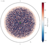 |
Fig. 1. Global distribution of 24 h, backward-in-time FTLE of solar surface flows (in inverse hour units) computed using photospheric velocity field maps of 29 November 2018, up to 60° from the disc centre. The green circle corresponds to a typical 30 Mm supergranule diameter. |
This network can be further highlighted by looking at the ridges of the FTLE field, or by emphasising the maxima of the field using an appropriate colormap. This results in maps of LCSs acting as a complex network of transport barriers on the timescale of consideration. In Fig. 2, we show such global maps for FTLE fields computed backward-in-time over different integration times, up to six days. This is, to the best of our knowledge, the first calculation of this type over such long integration times and large areas. The structures are remarkably long-lived, and simple visual inspection reveals their tendency to moderately expand in size as a function of time. We characterise this effect quantitatively in Sect. 4.3.
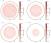 |
Fig. 2. From left to right and top to bottom: global solar-disc maps of attractive Lagrangian coherent structures imaged as ridges of maxima of the backward-in-time FTLE field, for different integration times of 1, 2, 3 and 6 days respectively. Increasingly small apodising windows are used for longer time integrations (from 60° opening for T = 24 h to 23.5° opening for T = 144 h) to avoid contamination by imprecise velocity measurements at the limb (see discussion in Sect. 2). |
4.2. LCS and the distribution of magnetic fields
Figures 3 and 4 show zooms of such maps on a region of 122 × 122 Mm2 (10° × 10°) at the (de-rotated) disc centre, over-imposed with SDO/HMI magnetograms. These zoomed maps do not only enable us to better appreciate the mesmerising structure of these patterns, they also show how much their fine-scale structure correlates with the magnetic network at the surface. As discussed by Yeates et al. (2012), on timescales of the order of the supergranulation timescale, LCS should be associated with regions of magnetic field accumulations. This is exactly what we observe here too: small-scale photospheric magnetic field concentrations appear to correlate extremely well with LCS derived from passive tracers. The results above (Figs. 1 and 2) therefore offer a striking new global-scale perspective on this phenomenon. Finally, Figs. 3 and 4 show the trajectories of a few selected tracers with remarkable excursions on the timescales of consideration. We discuss these in more detail in Sect. 5 in connection with magnetic dynamics and transport.
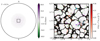 |
Fig. 3. Left: line-of-sight magnetic field Bz over the central 23.5° region, imaged with SDO/HMI 12 h after the beginning of the observation. Right: zoomed-in centre-disc region of 10° ×10° (frame in left plot) showing attractive LCS calculated for 12 h negative integration time (ridges of the negative-time FTLE field, red colormap), superimposed with passive tracer locations after 12 h positive integration time (black dots), and corresponding local Bz magnetograms (green/purple colormap). The coloured markers and lines tag 12 h (positive time) trajectories of a few selected tracers, see discussion in Sect. 5 and Fig. 7 below (visualisation continued for longer times in Fig. 4). |
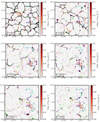 |
Fig. 4. Continuation of Fig. 3. From top left to bottom right: zoomed-in region (frame in Fig. 3, left) showing attractive LCS calculated for successive negative tracer integration times (red colormap), superimposed with passive tracer locations (black dots) and corresponding local Bz magnetograms (same green/purple colormap as in Fig. 3) at corresponding positive integration times. As mentioned in Sect. 3, tracers accumulate in attractive LCS. Throughout the sequence, LCS and tracer concentrations correlate well with the magnetic network and bright points, respectively. The coloured markers and lines tag (positive-time) trajectories of a few selected tracers: large symbols mark the initial position and current position for the time of integration of each plot, and small symbols the position for every intermediate 24 h (see discussion in Sect. 5 and Fig. 7). |
4.3. Spectrum, scales, and strength of the FTLE field
To be more quantitative, for any FTLE map such as shown in Fig. 1, we compute a typical peak scale of the distribution of FTLEs, corresponding to the wavelength of the LCS/transport barriers, as the integral scale of the FTLE field. To do this, we simply treat each FTLE field as a scalar field σT(θ, φ) over the sphere apodised by the visibility window, take its harmonic transform, compute the associated spherical harmonics spectrum Eσ(ℓ, T), and calculate the integral scale of the field, defined as
 (2)
(2)
This formula simply weighs each scale by its corresponding energetic spectral content, providing a weighted mean giving more weight to the scales at which the distribution of σT contains the most energy. The lower bound in the sum avoids contamination by the large-scale energetic content of the apodising window, with which the true field is convoluted in spectral space. The numerical technique used for the spectral harmonic decomposition of our data fields over apodised fields of views is described in detail in R17, where ample use of it was made to characterise the structure and scale of the turbulent flow itself. Here, we simply apply the same tool to FTLE fields.
Figure 5 shows the spherical harmonics spectra Eσ(ℓ, T) of FTLE fields for different target integration times, shown earlier in Fig. 2. As LCS form and evolve, their energy content and peak scale shifts towards larger scales, and the spectrum becomes steeper. By T = 24 h, the slope of the spectrum becomes stationary at intermediate scales, but the peak scale continues to increase monotonically on larger times.
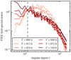 |
Fig. 5. Spherical harmonics spectra of the FTLE field for different target times. The spectra are normalised to one at the standard supergranulation angular degree scale ℓ = 120 (dashed vertical line) to highlight the pivot of the spectrum towards larger physical angular scales on longer times. |
The corresponding evolution of Lσ is shown in Fig. 6 as a function of the target time of integration of passive tracers. As this time increases, Lσ increases from 16 Mm at T = 6 h to 21 Mm at T = 72 h, and subsequently saturates. Thus, LCS, while acting as transport barriers, are not immutable in this kind of time-dependent flow unconstrained by horizontal boundaries3. Instead, they themselves appear to be highly dynamical structures that change in time as the flow evolves.
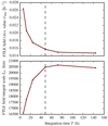 |
Fig. 6. Change as a function of the FTLE target integration time of the r.m.s. value and integral scale of FTLE distributions, derived from spherical harmonics spectra using Eq. (2). The dashed vertical line shows τSG = 48 h, the typical correlation time of supergranulation. |
Figure 6 also shows how the r.m.s. value of the FTLE field σT evolves with the integration time. This quantity indicates how particles diverge as a function of time. A fast initial divergence over a timescale of a few hours is initially observed (σrms ∼ 0.025 h−1, with peak values σmax ∼ 0.14 h−1 for T = 24 h corresponding to a shortest divergence timescale of just 8 h, see Fig. 1). This shorter timescale roughly corresponds to the time it takes for tracers to be swept by supergranulation-scale flows from a supergranulation cell centre to its periphery. On longer timescales, however, particles tend to get trapped/blocked in the LCS transport barriers associated with supergranule boundaries. As a result, the rate of relative divergence of their trajectories significantly decreases, as visible in Fig. 6, and appears to saturate at σrms ∼ 0.015 h−1.
Using the long-time asymptotic values reached by Lσ and σrms in Fig. 6, we can infer a first rough dimensional turbulent diffusion coefficient estimate, namely
 (3)
(3)
While this simple result should be treated with caution and should only be seen as an order of magnitude estimate, we point out that it provides an interesting connection between LCS, FTLEs and large-scale transport, which we study more quantitatively in the next section.
5. Statistical characterisation of turbulent transport
The previous section aimed at providing a phenomenological perspective on large-scale transport in the quiet photosphere, and it notably enabled us to pinpoint a global network of Lagrangian coherent structures associated with supergranulation-scale convection as a key physical pattern regulating horizontal turbulent diffusion in this convective fluid system. We now proceed to analyse the horizontal transport process on timescales of up to six days from a more classical statistical perspective, and subsequently attempt to interpret the results through the phenomenology outlined previously.
5.1. Statistics of tracer trajectories
To quantify turbulent transport, we focus on the central 23.5° region, whose velocity field can be reliably inferred throughout our 144 h sequence. We calculate the trajectories of 1024 × 1024 tracers initially placed on a cartesian grid at the centre of this region, with a resolution of 135 km. We first calculate the ensemble average (denoted by brackets) of the squared distance di, j2(T) = |xi, j(T)−xi, j(0)|2 travelled by each (i, j) tracer initially placed on this cartesian grid, as a function of the integration time. On general grounds, we expect
 (4)
(4)
with γ = 1 corresponding to a random walk diffusion regime, γ > 1 to an anomalous super-diffusion regime, and γ < 1 to an anomalous sub-diffusion regime. Using power-law fits to Eq. (4), we can then calculate a horizontal 2D-turbulence diffusion coefficient using a formula frequently used in the solar physics context (Monin & Yaglom 1971, see e.g. Hagenaar et al. (1999), Abramenko et al. (2011)),
 (5)
(5)
We note that this transport coefficient usually bears a residual dependence on T if γ ≠ 1, and that this expression also motivates a posteriori the specific expression used in Eq. (3) to estimate turbulent diffusion on the basis of the characteristic rate of tracers divergence and spatial scales obtained from our FTLE analysis.
We plot ⟨d2⟩(T) and D for our collection of advected tracers in Fig. 7. We obtain a reasonable power-law fit with γ = 1.09 for intermediate times comparable to τSG = 48 h, the typical correlation time of supergranulation. This corresponds to an almost-diffusive behaviour with a turbulent diffusion coefficient in the range D = 200 − 300 km2 s−1 (inset). A histogram of the distribution of distances travelled by tracers (Fig. 8) further illustrates the spread in distances travelled as a function of time, consistent with a diffusive process.
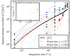 |
Fig. 7. Ensemble-averaged ⟨d2⟩ of the quadratic distance travelled by tracers as a function of time (solid dark red line), power law fits (lighter red and cream lines), and (inset) corresponding diffusion coefficients as determined by Eq. (5). The thin coloured lines with markers every 24 h show the history of d2 for individual tracers with larger-than-average excursions on long times. The surface trajectories of these tracers are shown with the same markers and colours in Figs. 3 and 4. |
On the longest times probed though, we find in Fig. 7 a slight increase in transport (γ = 1.57), corresponding to an enhanced diffusion coefficient D ≃ 400 km2 s−1. To understand the origins of this trend, we isolated a collection of tracers with larger-than-average excursions d from their initial positions. We over-plot d(T) for ten of these tracers in the figure using thin colour lines and symbols, and further trace their trajectories at the solar surface in Figs. 3 and 4. A careful examination of these figures reveals that most of these tracers experience secondary transport kicks at a time between 24 h and 72 h comparable to τSG. These kicks appear to be associated with the regeneration of the supergranulation flow and the emergence of new “explosive granules” (Roudier et al. 2016) that structure supergranules, leading to a transient, more ballistic-like energetic super-diffusive behaviour. Since the average statistical trend at the largest times probed here is dominated by the small collection of tracers in this “non-thermal” tail of the distribution shown in Fig. 8, we argue, consistent with the standard picture of a random walk, that such individual kicks are simply random-walk events associated with the regeneration of the supergranulation flow, and that the accumulation of such events on timescales much larger than τSG would likely result on long times in an average diffusive-like behaviour. Accordingly, we conjecture that the statistics of ⟨d2⟩ should eventually settle in such a large-scale turbulent diffusion regime if we could track tracers trajectories for even longer times than we did here to reach a better timescale separation with the typical correlation time of the flow. Despite our best efforts to maximise the consecutive time of observation, reaching this regime unfortunately currently remains impossible, due to the observing limitations stressed in the Introduction and in Sect. 2.4. For this reason, we stress that the specific values of γ and D given above should not be taken as precision measurements. Instead, the two sets of values inferred in Figure 7 are best understood as a lower and upper bounds on the exact transport coefficients and scaling exponents.
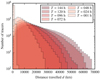 |
Fig. 8. Time evolution of the histogram distribution of distances travelled by tracers. The tracers showcased by markers in Figs. 3–4 and Fig. 7 all belong to the tail of the distribution at T = 144 h. |
With respect to this point, close examination of Figs. 3 and 4 also reveals that some magnetic concentrations at the surface are subject to the exact same dynamics as these outlier tracers. For instance, an intense violet magnetic concentration located at (2° E, 2.3° S) at T = 96 h gets pushed further south in exactly the same way as the tracers tagged with red and cyan triangles between T = 96 h and T = 120 h, at which time the position of the two tracers almost coincides with that of the magnetic element. The same remark applies at T = 120 h to the green magnetic concentration located at (0.5° W, 2.2° N), and to the tracer tagged by a yellow pentagon. This provides further confirmation that the dynamics of tracers and magnetic fields are strongly correlated, and that both are subject to the same kind of average transport and individual transport events/kicks.
5.2. Ink spot experiment
To complement the previous results, and in the spirit of approaching the problem from a large-scale statistical point of view, we finally present a slightly different characterisation of transport by photospheric flows. The idea is to mimic a classical ink spot molecular diffusion experiment in the lab, whereby a circular ink spot is carefully released in water, and its radius subsequently expands diffusively. To do this, we delimit a circular patch of tracers in the initially cartesian grid of tracers (as in Sect. 4, we use a large tracers grid covering the entire solar surface here). We then measure the evolution of their average squared distance from the centre of the spot
 (6)
(6)
where (xc, yc) are the central coordinates of the spot on the CCD grid and N is the number of tracers initially within a radius R0 of the spot centre. For a diffusive process, a spot of initial radius R0 will diffuse on a timescale τD = R02/D, where D is the diffusion coefficient. For the experiment to be meaningful, we should pick R0 small enough that τD is smaller than, or at most of the order of the observation period, but also large enough that the circular spot itself encompasses at least one typical supergranule structure. Indeed, a very large spot would barely start to diffuse on the available time of observation, while a very small one would not feel the statistical effect of turbulent kicks and would also not contain enough tracers to construct a meaningful statistics. In what follows, we chose R0 = 28.7 Mm, which corresponds to an angle with respect to the Sun centre of 2.35°, one-tenth of the opening of the apodising window used for the continuous six-day observation. Based on our earlier estimate for D, such a spot should diffuse on a typical timescale of a month, so we expect to be able to measure the beginning of the diffusion process using our six-day sequence.
A spot of initially this size contains ∼1380 tracers for our grid of tracers and it samples the flow of only a handful of independent supergranules giving relatively noisy results. To improve the statistics, we therefore replicate the measurement in Eq. (6) for as many spots as possible, packing the 23.5° observation window with non-overlapping circular spots whose centres are contained initially within an opening 21.15° = 23.5° −2.35° angle from the solar disc centre. For the chosen R0, this gives us a statistics of 60 spots from which we can calculate  , a spot-ensemble average of Rspot2. Because the diffusion process takes a few hours to develop, we parameterise the evolution as
 (7)
(7)
In Fig. 9, we plot  as a function of the integration time of tracers, and a corresponding power law fit of the evolution for times longer than 24 h. While the observed statistics is neither an exact power law, nor exactly diffusive, diffusion still appears to be a very reasonable first approximation overall, and the scaling exponent γ = 1.15 is very similar to γ = 1.09 obtained with the first method used in Sect. 5.1. As in Fig. 7, we also observe that transport is slightly enhanced on late times, for the same reasons. Figure 10 further shows the histogram distribution, as a function of time, of the distance of all the tracers considered in the analysis from their relative spot centre. The results illustrate the diffusion-like spread of the averaged spot.
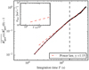 |
Fig. 9. Time evolution of the ensemble-average normalised radius of circular spots of tracers (solid dark red line, see Eq. (7)), and corresponding power-law fit. |
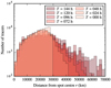 |
Fig. 10. Time evolution of the histogram distribution of distances travelled by tracers initially enclosed within circular spots of tracers of radius 30 000 km, with respect to their relative spot centres. Together with Fig. 9, the plot highlights the turbulent diffusive spread of tracers. |
Using this analysis, we can now estimate a large-scale diffusion coefficient from the power law fit in Fig. 9. For consistency and comparison with the method used in Sect. 5.1, we use again Eq. (5) for this purpose, applied here to  instead of ⟨d2⟩. The results, shown in the inset of Fig. 9, give Dspot ≃ 200 km2 s−1 for T = 48 h, consistent with the value obtained by the first method in Sect. 5.1.
6. Conclusions and discussion
6.1. Main conclusions
In this paper, we have studied large-scale transport by convection flows in the solar photosphere from an observational perspective, using a Lagrangian passive tracer modelling approach to characterise turbulent diffusion and the formation of dynamical structures and patterns affecting this transport process.
In Sect. 4, we applied finite time Lyapunov exponents (FTLEs) and Lagrangian coherence structure (LCS) analysis techniques to large field of views covering a significant fraction of the solar disc, for unprecedented continuous periods of tracer tracking of up to six days. The large-scale maps we obtained reveal a clear and robust emergent dynamical LCS pattern tiling the solar surface isotropically at supergranulation scales. These results provide a new global perspective, rooted in observational data, of the dynamical interplay between order and chaos at the solar surface. In particular, by transiently accumulating particles and magnetic fields, Lagrangian coherent structures appear to regulate large-scale turbulent surface diffusion in the quiet Sun on long timescales. We also found that characterising their associated basic statistical properties (space and time scales) is sufficient to provide a correct preliminary dimensional order of magnitude estimate of the large-scale turbulent diffusivity.
A more quantitative statistical analysis of large-scale diffusion was presented in Sect. 5 using two different methods: a direct statistical analysis of tracers trajectories, which notably allowed us to pinpoint the role of “large-scale” flow kicks in driving the transport on long timescales, and an analogue to an ink spot molecular diffusion laboratory experiment. Although they may not capture the diffusion processes on precisely the same spatial scales due to their different methodologies and to the specific choice of R0 in the ink spot experiment, both analyses point to an effective mean horizontal turbulent diffusivity coefficient D = 2 − 3 × 10⁸ m2 s−1 on the longest timescales of six days probed (with an upper bound D = 4 × 10⁸ m2 s−1 on the longest timescale probed, see Fig. 7). We argued that an analysis on even longer times (much larger than the correlation timescale of supergranulation) would be desirable to make the convergence to an asymptotic, long-time statistical diffusion regime more apparent, but that such an analysis cannot be easily conducted currently considering observational constraints. Another possibility to further characterise the process, left for future work, would be to calculate probability distribution functions of first passage times of tracers.
6.2. Comparison with previous work
The passive tracers advection analysis presented in this paper bears some similarities with a previous analysis of this kind conducted by Roudier et al. (2009) on Hinode data on a 48 h timescale. The authors derived a diffusion coefficient D ≃ 430 km2 s−1, broadly consistent with, but on the higher end of our own estimates. It is possible that the timescale they probed was not long enough to obtain a converged long-time diffusion coefficient, with the statistics being dominated by shorter-time, super-diffusive ballistic advection within supergranules. The present analysis, conducted on times larger than the typical supergranulation lifetime τSG and on significantly larger fields of views, offers a significant statistical improvement in this respect.
Our results can also be compared with solar studies involving the tracking of magnetic elements. We argued that magnetic transport is overall well captured by the dynamics of virtual passive tracers/corks. The main benefits of the latter, we recall, is that they can be integrated for longer times, provide better statistics and do not suffer from the issue of cancellation/merging effects (see e.g. Iida 2016, for a discussion). As mentioned in the introduction, all studies of this kind so far have focused on smaller fields of views and smaller timescales than the present study. Where the timescales of these studies overlap with ours, we find good agreement with our results. For instance, Hagenaar et al. (1999) derived D = 200 − 250 km2 s−1 for magnetic tracking times in the 19 − 45 h range; Giannattasio et al. (2013, 2014) report a slightly hyper-diffusive regime with D = 100 − 400 km2 s−1 on supergranulation scales for a few hours. Most other observational solar magnetic turbulent diffusion studies in the literature (e.g. Berger et al. 1998; Utz et al. 2010; Abramenko et al. 2011; Manso Sainz et al. 2011; Jafarzadeh et al. 2014; Yang et al. 2015; Agrawal et al. 2018) have been focused on intra-supergranular/inter-network transport on significantly smaller times (103 − 105 s) and spatial scales of a few megametres at most (see Schrijver et al. (1996), Bellot Rubio & Orozco Suárez (2019) for reviews). They typically obtain diffusion coefficients smaller than 100 km2 s−1 that likely correspond to transport by shorter-lived, smaller-scale structures such as granules or explosive granules, with only a minor effect of weaker, but much longer-lived supergranulation-scale flows on such short timescales. These studies therefore differ in both scales, scope, goal and spirit from our study, which preferentially targets effective large-scale transport on times comparable to, or larger than the typical supergranulation lifetime τSG = 48 h, which we believe is the appropriate limit to gauge the turbulent diffusion relevant to the large-scale solar dynamo problem.
6.3. Implications for solar dynamo modelling
Our long-time observational estimates of turbulent diffusivity, D ≃ 2 − 3 × 10⁸ m2 s−1 obtained in Sect. 5, may be used to pin, at the solar photosphere, the profiles of horizontal turbulent magnetic diffusivity used for instance in mean-field models of the solar dynamo (Hazra et al. 2023). If our results hold, some existing models might slightly underestimate this mode of transport (e.g. Rempel 2006, who used 108 m2 s−1 at the surface), while others use a turbulent diffusivity value entirely consistent with our observational estimate (e.g. D ≃ 2.5 × 10⁸ m2 s−1 in Cameron et al. (2010)). On the other hand, some older flux-transport kinematic dynamo models (Sheeley 1992, 2005, see Schrijver et al. (1996) for a discussion) seemed to require a significantly larger turbulent diffusion coefficient, up to D ≃ 6 × 10⁸ m2 s−1, to produce sensible solar dynamo results. Such a large value is not consistent with even our upper-limit, enhanced transport estimates, D ≃ 4 × 10⁸ m2 s−1, obtained on the longest times probed, and associated with transiently re-accelerated “tail particles” (see inset of Fig. 7 and related discussion in Sect. 5). To be sustained on asymptotically long-times, such a large coefficient would require a significant transport regime change on longer timescales than the six days probed here. Such a dynamical effect is hard to envision at the surface at least, considering that our study already encompasses the main effects of supergranulation-scale convection, the most energetic large-scale flow structure contributing to turbulent transport at the surface.
Further mean-field solar dynamo modelling work by Lemerle et al. (2015) (see their Fig. 8), highlighted in a recent review on surface flux transport by Yeates et al. (2023), found a degeneracy between turbulent diffusivity and meridional flow amplitude parameters on the results of flux-transport dynamo models, which may somehow help to solve this problem. We believe that the multi-pronged statistical characterisation of the horizontal turbulent diffusivity at the photosphere developed in the present paper is sufficiently robust to help lift this degeneracy: our result, D ≃ 2 − 3 × 10⁸ m2 s−1, is very close to the turbulent diffusivity value associated with the maximum fitness contours obtained by Lemerle et al. (2015) in the turbulent diffusivity-meridional flow amplitude plane.
Finally, we note that transport coefficients derived from global numerical simulations of solar MHD convection also seem consistent with our observational estimates (e.g. Fig. 11 of Simard et al. (2016) for the βφφ transport coefficient corresponding to our observational measurement of the horizontal diffusivity), although they might still slightly underestimate the vigour of the convection at supergranulation scales, and the associated diffusivity.
6.4. Connection with the solar magnetic network, atmosphere and solar wind
It is tempting to conjecture that the prominent global emergent dynamical pattern tiling the surface of the Sun, singled out in this work and best illustrated by Fig. 1, plays a major role in structuring the magnetic interactions between the interior, or at least the subsurface layers of the Sun driving the small-scale surface dynamo, its atmosphere, and possibly also the solar wind. The possible connection of the LCS loci of photospheric magnetic field accumulation with coronal heating has already been pointed out by Yeates et al. (2012). Our new global characterisation reveals the conspicuity, robustness and full extent of this dynamical LCS pattern over the whole solar disc, reinforcing this hypothesis. In this respect, our analysis may also provide new insights into the origin and mechanisms underlying a possible connection, suggested by Fargette et al. (2021), between supergranulation and solar wind magnetic switchbacks encountered by the Parker Solar Probe (Kasper et al. 2019; Bale et al. 2019).
6.5. A new “experimental” measurement of turbulent transport
Moving on to a more fundamental complex physics and fluid-dynamical perspective, we note that turbulent diffusion effects have been observed in various experimental MHD flows, such as the Perm, Wisconsin and VKS dynamo experiments (Frick et al. 2010; Rahbarnia et al. 2012; Miralles et al. 2013), all at relatively large kinetic Reynolds numbers Re = O(106) but rather small magnetic Reynolds numbers (Rm < 100) not representative of astrophysical regimes such as encountered in planets, stars and galaxies. By using “the Sun as a fluid dynamics lab”, our results offer a new, and possibly unique “experimental”, in situ characterisation of the emergence on times comparable to, or longer than a typical flow correlation time, of turbulent diffusion in stochastic flows with both large kinetic and magnetic Reynolds numbers (Re = O(1010), Rm = O(104) at the solar surface).
6.6. The pitfalls of mixing-length arguments
Looking at the results from a broader perspective than just the solar context to benefit from the insights of the study of an astrophysical system resolved in both space and time, it is also an interesting exercise to ask why the value of the turbulent diffusivity we obtained is what it is in this system. If the transport is indeed dominated by supergranulation-scale flows, naïvely (by a mixing length argument) one could have expected a transport coefficient of the order of a fraction (typically 1/4 in 2D) of RSGVSG,
 (8)
(8)
where we have used RSG ≃ 1.5 × 10⁴ km, and VSG ≃ 0.4 km s−1 (Rincon & Rieutord 2018), and we have introduced the nonlinear turnover time at the supergranulation scale τNL, SG = RSG/VSG ≃ 8 h, which is the sweeping time for a passive tracer to be advected from the centre to the boundary of a supergranule cell. This mixing-length estimate is an order of magnitude higher than our experimental-observational determination. The reason lies in that we have naïvely used, in the expression above, the turnover time of the flow τNL, SG, instead of its correlation time, τSG, which is closer to 48 h. If we repeat the calculation in Eq. (8) with this time instead, we find D = 2.6 × 10⁸ m2 s−1, which is now remarkably consistent with our detailed statistical analysis.
The reason why the correlation time of the flow is the relevant quantity to use in a mixing length estimate here is because tracers remain stuck at the boundary of supergranules for a time of the order of τSG after they have been advected there on the much shorter τNL, SG time. Hence, their effective “random walk” velocity is not VSG = 0.4 km s−1, but the much smaller VSG × (τNL, SG/τSG)≃70 m s−1. This simple, yet subtle difference finds its roots in the very structure of the flow.
The conclusion of this phenomenological argument is therefore that the structure of a turbulent flow matters a lot when it comes to correctly estimating the magnitude of large-scale turbulent transport. In the example at hand, we showed that the global surface network of transport barriers and LCS at supergranulation scales, vividly illustrated in Fig. 1, plays a key role in the regulation of the effective large-scale transport. We believe that this conclusion pertains to many if not all astrophysical flows, and therefore call for caution with back-of-the-envelope estimates of turbulent transport coefficients based on dimensional arguments, for instance because the correlation time of the flow can significantly differ from its turnover time. In the case of solar surface convection, large-scale structures at the injection scale persist for quite a long time, so that the Strouhal number of the flow, St = τcorr/τNL, is of the order of 5–6, with significant consequences for the effective turbulent diffusivity.
6.7. Perspectives
The focus of this paper has deliberately been restricted to a subset of all physical solar dynamical transport and large-scale organisation phenomena to which the techniques developed in this work may be applied at global scales. Further investigations of this kind, of possible rotational effects, latitudinal dependencies of turbulent diffusivity, global-scale convection (Hathaway et al. 2013, Ballot & Roudier in prep.), meridional circulation (Roudier et al. 2018), and of the statistical implications of magnetic flux emergence and further transport at the photosphere (Hathaway & Rightmire-Upton 2012) for the energetics of the upper solar layers (Yeates et al. 2012), would undoubtedly prove very instructive too, and are left for future work.
More broadly, as exemplified by the discussion above, the study of the extreme fluid dynamical system that is the Sun, with the unique benefits in astrophysics of a large spatial and temporal resolution, can still teach us valuable lessons for the future modelling of unresolved astrophysical systems, such as stars or accretion discs, where turbulent flows driven by different hydrodynamic or MHD instabilities also likely play a key role in the overall dynamical and energetic regulation of the system.
The two FTLEs of the flow on the surface are probably close to two of the three FTLEs of the full 3D flow, because the photospheric velocity field at the large scales considered in this paper is strongly anisotropic with respect to the radial direction (R17).
In marine dynamics for instance, LCS can be laminar patterns whose geometry is shaped by coastal/bay topography, and they can be extremely stable over time, leading for example to accumulation of pollutants in particular areas, see e.g. Lekien et al. (2005).
Acknowledgments
We thank Peter Haynes and Yves Morel for several interesting conversations and for their invitation to discuss and present a preliminary version of the results at the 2019 TEASAO workshop in the beautiful surroundings of the Saint-Férréol lake, and Michael Nastac for a useful discussion on the theory of anomalous transport scaling in turbulence during an astrophysical plasma workshop organised at the Wolfgang Pauli Institute in Vienna, whose hospitality is gratefully acknowledged. We also thank Nathanaël Schæffer for his assistance with the SHTns library (Schaeffer 2013), the SDO/HMI data provider JSOC and the HMI/SDO team members for their hard work. In particular, we are grateful to P. Scherrer, S. Couvidat and J. Schou for sharing information regarding the calibration and removal of systematics of HMI Doppler data. This work was granted access to the HPC resources of CALMIP under the allocation 2011-[P1115]. We thank Nicolas Renon for his assistance with the parallelisation of the CST code. This work was supported by COFFIES, NASA Grant 80NSSC20K0602.
References
- Abramenko, V. I., Carbone, V., Yurchyshyn, V., et al. 2011, ApJ, 743, 133 [NASA ADS] [CrossRef] [Google Scholar]
- Agrawal, P., Rast, M. P., Gošić, M., Bellot Rubio, L. R., & Rempel, M. 2018, ApJ, 854 [Google Scholar]
- Amari, T., Luciani, J.-F., & Aly, J.-J. 2015, Nature, 522, 188 [NASA ADS] [CrossRef] [Google Scholar]
- Bale, S. D., Badman, S. T., Bonnell, J. W., et al. 2019, Nature, 576, 237 [NASA ADS] [CrossRef] [Google Scholar]
- Bellot Rubio, L., & Orozco Suárez, D. 2019, Liv. Rev. Sol. Phys., 16, 1 [Google Scholar]
- Berger, T. E., Löfdahl, M. G., Shine, R. A., & Title, A. M. 1998, ApJ, 506, 439 [NASA ADS] [CrossRef] [Google Scholar]
- Brun, A. S., & Browning, M. K. 2017, Liv. Rev. Sol. Phys., 14, 4 [Google Scholar]
- Brunton, S. L., & Rowley, C. W. 2010, Chaos, 20, 017503 [NASA ADS] [CrossRef] [Google Scholar]
- Cameron, R. H., Jiang, J., Schmitt, D., & Schüssler, M. 2010, ApJ, 719, 264 [NASA ADS] [CrossRef] [Google Scholar]
- Charbonneau, P. 2014, ARA&A, 52, 251 [NASA ADS] [CrossRef] [Google Scholar]
- Chian, A. C.-L., Rempel, E. L., Aulanier, G., et al. 2014, ApJ, 786, 51 [NASA ADS] [CrossRef] [Google Scholar]
- DeGrave, K., & Jackiewicz, J. 2015, Sol. Phys., 290, 1547 [Google Scholar]
- Duvall, T. L., & Hanasoge, S. M. 2013, Sol. Phys., 287, 71 [Google Scholar]
- Duvall, T. L., Hanasoge, S. M., & Chakraborty, S. 2014, Sol. Phys., 289, 3421 [Google Scholar]
- Fargette, N., Lavraud, B., Rouillard, A. P., et al. 2021, ApJ, 919, 96 [NASA ADS] [CrossRef] [Google Scholar]
- Frick, P. A., Noskov, V. I., Denisov, S. A., & Stepanov, V. A. 2010, Phys. Rev. Lett., 105, 184502 [Google Scholar]
- Giannattasio, F., Del Moro, D., Berrilli, F., et al. 2013, ApJ, 770, L36 [NASA ADS] [CrossRef] [Google Scholar]
- Giannattasio, F., Stangalini, M., Berrilli, F., Del Moro, D., & Bellot Rubio, L. 2014, ApJ, 788, 137 [NASA ADS] [CrossRef] [Google Scholar]
- Gizon, L., Birch, A. C., & Spruit, H. C. 2010, ARA&A, 48, 289 [Google Scholar]
- Green, M. A., Rowley, C. W., & Haller, G. 2007, J. Fluid Mech., 572, 111 [NASA ADS] [CrossRef] [Google Scholar]
- Greer, B. J., Hindman, B. W., Featherstone, N. A., & Toomre, J. 2015, ApJ, 803, L17 [Google Scholar]
- Hagenaar, H. J., Schrijver, C. J., Title, A. M., & Shine, R. A. 1999, ApJ, 511, 932 [CrossRef] [Google Scholar]
- Haller, G. 2001, Phys. Fluids, 13, 3365 [Google Scholar]
- Hanasoge, S. M., Duvall, T. L., & Sreenivasan, K. R. 2012, Proc. Natl. Acad. Sci., 109, 11928 [Google Scholar]
- Hanasoge, S., Gizon, L., & Sreenivasan, K. R. 2016, Ann. Rev. Fluid Mech., 48, 191 [Google Scholar]
- Hart, A. B. 1954, MNRAS, 114, 17 [Google Scholar]
- Hathaway, D. H., & Rightmire-Upton, L. 2012, Am. Astron. Soc. Meeting Abstr., 220, 110.06 [NASA ADS] [Google Scholar]
- Hathaway, D. H., Beck, J. G., Bogart, R. S., et al. 2000, Solar Phys., 193, 299 [Google Scholar]
- Hathaway, D. H., Upton, L., & Colegrove, O. 2013, Science, 342, 1217 [NASA ADS] [CrossRef] [Google Scholar]
- Hathaway, D. H., Teil, T., Norton, A. A., & Kitiashvili, I. 2015, ApJ, 811, 105 [Google Scholar]
- Hazra, G., Nandy, D., Kitchatinov, L., & Choudhuri, A. R. 2023, Space Sci. Rev., 219, 39 [Google Scholar]
- Hotta, H., Rempel, M., & Yokoyama, T. 2014, ApJ, 786, 24 [NASA ADS] [CrossRef] [Google Scholar]
- Iida, Y. 2016, J. Space Weather Space Clim., 6, A27 [NASA ADS] [CrossRef] [EDP Sciences] [Google Scholar]
- Jafarzadeh, S., Cameron, R. H., Solanki, S. K., et al. 2014, A&A, 563, A101 [NASA ADS] [CrossRef] [EDP Sciences] [Google Scholar]
- Kashyap, S. G., & Hanasoge, S. M. 2021, ApJ, 916, 87 [NASA ADS] [CrossRef] [Google Scholar]
- Kasper, J. C., Bale, S. D., Belcher, J. W., et al. 2019, Nature, 576, 228 [Google Scholar]
- Langfellner, J., Gizon, L., & Birch, A. C. 2015, A&A, 581, A67 [NASA ADS] [CrossRef] [EDP Sciences] [Google Scholar]
- Leighton, R. B., Noyes, R. W., & Simon, G. W. 1962, ApJ, 135, 474 [NASA ADS] [CrossRef] [Google Scholar]
- Lekien, F., & Coulliette, C. 2007, Phil. Trans. R. Soc. Lond. Ser. A, 365, 3061 [Google Scholar]
- Lekien, F., & Ross, S. D. 2010, Chaos, 20, 017505 [NASA ADS] [CrossRef] [Google Scholar]
- Lekien, F., Coulliette, C., Mariano, A. J., et al. 2005, Physica D, 210, 1 [Google Scholar]
- Lemerle, A., Charbonneau, P., & Carignan-Dugas, A. 2015, ApJ, 810, 78 [NASA ADS] [CrossRef] [Google Scholar]
- Manso Sainz, R., Martínez González, M. J., & Asensio Ramos, A. 2011, A&A, 531, L9 [NASA ADS] [CrossRef] [EDP Sciences] [Google Scholar]
- Miesch, M. S. 2005, Liv. Rev. Sol. Phys., 2, 1 [Google Scholar]
- Miralles, S., Bonnefoy, N., Bourgoin, M., et al. 2013, Phys. Rev. E, 88, 013002 [Google Scholar]
- Monin, A. S., & Yaglom, A. M. 1971, Statistical Fluid Mechanics: Mechanics of Turbulence (MIT Press) [Google Scholar]
- Nordlund, Å., Stein, R. F., & Asplund, M. 2009, Liv. Rev. Sol. Phys., 6, 2 [Google Scholar]
- November, L. J. 1989, ApJ, 344, 494 [CrossRef] [Google Scholar]
- November, L. J., & Simon, G. W. 1988, ApJ, 333, 427 [Google Scholar]
- Orozco Suárez, D., Katsukawa, Y., & Bellot Rubio, L. R. 2012, ApJ, 758, L38 [CrossRef] [Google Scholar]
- Rahbarnia, K., Brown, B. P., Clark, M. M., et al. 2012, ApJ, 759, 80 [NASA ADS] [CrossRef] [Google Scholar]
- Rempel, M. 2006, ApJ, 647, 662 [NASA ADS] [CrossRef] [Google Scholar]
- Rieutord, M., Roudier, T., Ludwig, H., Nordlund, Å., & Stein, R. 2001, A&A, 377, L14 [NASA ADS] [CrossRef] [EDP Sciences] [Google Scholar]
- Rieutord, M., Roudier, T., Roques, S., & Ducottet, C. 2007, A&A, 471, 687 [NASA ADS] [CrossRef] [EDP Sciences] [Google Scholar]
- Rieutord, M., Meunier, N., Roudier, T., et al. 2008, A&A, 479, L17 [NASA ADS] [CrossRef] [EDP Sciences] [Google Scholar]
- Rieutord, M., Roudier, T., Rincon, F., et al. 2010, A&A, 512, A4 [NASA ADS] [CrossRef] [EDP Sciences] [Google Scholar]
- Rincon, F., & Rieutord, M. 2018, Liv. Rev. Sol. Phys., 15 [Google Scholar]
- Rincon, F., Roudier, T., Schekochihin, A. A., & Rieutord, M. 2017, A&A, 599, A69 [NASA ADS] [CrossRef] [EDP Sciences] [Google Scholar]
- Roudier, T., Rieutord, M., Malherbe, J. M., & Vigneau, J. 1999, A&A, 349, 301 [NASA ADS] [Google Scholar]
- Roudier, T., Rieutord, M., Brito, D., et al. 2009, A&A, 495, 945 [NASA ADS] [CrossRef] [EDP Sciences] [Google Scholar]
- Roudier, T., Rieutord, M., Malherbe, J. M., et al. 2012, A&A, 540, A88 [NASA ADS] [CrossRef] [EDP Sciences] [Google Scholar]
- Roudier, T., Rieutord, M., Prat, V., et al. 2013, A&A, 552, A113 [NASA ADS] [CrossRef] [EDP Sciences] [Google Scholar]
- Roudier, T., Malherbe, J. M., Rieutord, M., & Frank, Z. 2016, A&A, 590, A121 [NASA ADS] [CrossRef] [EDP Sciences] [Google Scholar]
- Roudier, T., Švanda, M., Ballot, J., Malherbe, J. M., & Rieutord, M. 2018, A&A, 611, A92 [NASA ADS] [CrossRef] [EDP Sciences] [Google Scholar]
- Roudier, T., Ballot, J., Malherbe, J. M., & Chane-Yook, M. 2023, A&A, 671, A98 [NASA ADS] [CrossRef] [EDP Sciences] [Google Scholar]
- Schaeffer, N. 2013, Geochem. Geophys. Geosyst., 14, 751 [NASA ADS] [CrossRef] [Google Scholar]
- Scherrer, P. H., Schou, J., Bush, R. I., et al. 2012, Sol. Phys., 275, 207 [Google Scholar]
- Schou, J., Scherrer, P. H., Bush, R. I., et al. 2012, Sol. Phys., 275, 229 [Google Scholar]
- Schrijver, C. J., Shine, R. A., Hagenaar, H. J., et al. 1996, ApJ, 468, 921 [NASA ADS] [CrossRef] [Google Scholar]
- Shadden, S. C., Lekien, F., & Marsden, J. E. 2005, Physica D, 212, 271 [Google Scholar]
- Sheeley, N. R. J. 1992, in The Solar Cycle, ed. K. L. Harvey, ASP Conf. Ser., 27, 1 [Google Scholar]
- Sheeley, N. R. 2005, Liv. Rev. Sol. Phys., 2, 5 [NASA ADS] [Google Scholar]
- Shine, R. A., Simon, G. W., & Hurlburt, N. E. 2000, Sol. Phys., 193, 313 [NASA ADS] [CrossRef] [Google Scholar]
- Simard, C., Charbonneau, P., & Dubé, C. 2016, Adv. Space Res., 58, 1522 [NASA ADS] [CrossRef] [Google Scholar]
- Simon, G. W., & Shine, R. A. 2004, BAAS, 36, 712 [NASA ADS] [Google Scholar]
- Švanda, M. 2012, ApJ, 759, L29 [Google Scholar]
- Švanda, M., Zhao, J., & Kosovichev, A. G. 2007, Sol. Phys., 241, 27 [Google Scholar]
- Taylor, G. I. 1922, Proc. Lon. Math. Soc., 2, 196 [Google Scholar]
- Toomre, J., & Thompson, M. J. 2015, Space Sci. Rev., 196, 1 [Google Scholar]
- Utz, D., Hanslmeier, A., Muller, R., et al. 2010, A&A, 511, A39 [NASA ADS] [CrossRef] [EDP Sciences] [Google Scholar]
- Williams, P. E., Pesnell, W. D., Beck, J. G., & Lee, S. 2014, Sol. Phys., 289, 11 [Google Scholar]
- Yang, Y., Ji, K., Feng, S., et al. 2015, ApJ, 810, 88 [NASA ADS] [CrossRef] [Google Scholar]
- Yeates, A. R., Hornig, G., & Welsch, B. T. 2012, A&A, 539, A1 [Google Scholar]
- Yeates, A. R., Cheung, M. C. M., Jiang, J., Petrovay, K., & Wang, Y.-M. 2023, Space Sci. Rev., 219, 31 [CrossRef] [Google Scholar]
Appendix A: Computation of Finite-Time Lyapunov exponents
A.1. Computation of Lagrangian tracers trajectories
The trajectories of Lagrangian tracers (“corks”) in the (x, y) plane are determined as follows: a cartesian grid of tracers is initially generated in the plane. The time history of the (x, y) projection of the photospheric velocity field u(xi, yj) = (ux(xi, yj),uy(xi, yj)), determined via the CST algorithm every 30 min, is then used to integrate their position in that plane for a target time T ranging from several hours to several days, by means of numerical integration of an advection equation implemented through the python function odeint. The integrator internally sets an adaptive timestep shorter than the time between successive velocity snapshots. At each such timestep, the velocity field at the exact current location of each tracer is interpolated using the running snapshot of the velocity field on the cartesian grid, thanks to the python function RectBivariateSpline. Using the same velocity field snapshot during 30 min intervals is a reasonable assumption, given that the smallest spatial scales of the photospheric flow inferred via the CST are of the order of 2.5 Mm, and their timescale is of the order of 30 min to 1 hour. Also, the resolution of the tracers grid on which a FTLE field is to be computed can be finer than the flow itself. Using a high-resolution grid of tracers is in fact essential to identify Lagrangian coherent structures and accurately compute invariant manifolds and transport barriers even when the flow is large-scale (Lekien et al. 2005). For global maps, we used a cartesian grid of up to 1024 × 1024 tracers encapsulating the full solar disc. This maximal resolution corresponds to an initial spacing between tracers of the order of 1.5 Mm close to the disc centre. The precision of the integration of the tracers trajectories, specified to the numerical integrator, is of the order of 0.3 Mm (in Sect. 5 we also used a much finer local grid of 1024 × 1024 tracers encompassing 10° ×10° only). The collection of trajectories integrated in the CCD plane then serves as a basis for the computation of FTLE on the sphere, as explained below.
A.2. FTLE in a 2D plane
The Lagrangian trajectory x(t) = (x(t),y(t)) of a passive tracer in a 2D plane fluid flow u(x, t) is determined by its initial position x(t = 0) = x0 and the differential equation of motion
 (A.1)
(A.1)
Introducing the flow map for a target integration time T
 (A.2)
(A.2)
and its Jacobian dϕT/dx0, we form the Cauchy-Green deformation tensor
 (A.3)
(A.3)
The FTLE σT(x0) of the flow at x0 is given by
 (A.4)
(A.4)
where λmax is the largest eigenvalue of Δ(x0).
In practice, the matrix representation J of dϕT/dx0 is estimated at each interior point (xi, yj) of the cartesian grid on which the tracers are placed at t = 0, using a centred finite difference formula. Using the short-hand notation xi, j(t)≡x(t, x0 = (xi, yj)), we have
 (A.5)
(A.5)
from which Δ=JTJ follows. The FTLE field σT(xi, yj) is finally obtained via Eq. (A.4) by diagonalising Δ at each grid point.
A.3. Mapping to the sphere
The FTLE of the flow on the sphere is inferred using basically the same algorithm presented above, except that a mapping between the real separations between the tracers and the projected ones in the plane of the sky/satellite CCD must be introduced. The theoretical formalism is described in Lekien & Ross (2010), as well as an example of application on the sphere. The formulae needed to compute FTLEs on the sphere for our particular problem are given below.
To perform the mapping, we introduce the out-of-plane distance z between a point on the solar surface and the plane parallel to the CCD plane and passing through the centre of the Sun,
 (A.6)
(A.6)
where R⊙ is a fiducial photospheric solar radius. The transformation between the solar disc D⊙ and spherical solar surface manifold ℳ is then given by the diffeomorphism
 (A.7)
(A.7)
Using these definitions, the FTLE field on the sphere is obtained along the exact same lines as in Appendix A.2, except that a more general form of the deformation tensor accounting for the projection effects must be used, namely
 (A.8)
(A.8)
with
 (A.9)
(A.9)
J is the Jacobian matrix in the projection plane, computed at each grid point via Eq. (A.5) using the projected tracers trajectories. R(x) is a coordinate-dependent upper-triangular matrix obtained by QR decomposition of the derivative of β−1. Its explicit expression for our particular problem is
 (A.10)
Since the particles move on the sphere between t = 0 and the target time t = T, the projection effects at T are different from those at the initial time. This explains why R is evaluated at the final position x(T) on the left of J in Eq. (A.9) and at the initial position x(0) on its right.
All Figures
|
Fig. 1. Global distribution of 24 h, backward-in-time FTLE of solar surface flows (in inverse hour units) computed using photospheric velocity field maps of 29 November 2018, up to 60° from the disc centre. The green circle corresponds to a typical 30 Mm supergranule diameter. |
| In the text | |
|
Fig. 2. From left to right and top to bottom: global solar-disc maps of attractive Lagrangian coherent structures imaged as ridges of maxima of the backward-in-time FTLE field, for different integration times of 1, 2, 3 and 6 days respectively. Increasingly small apodising windows are used for longer time integrations (from 60° opening for T = 24 h to 23.5° opening for T = 144 h) to avoid contamination by imprecise velocity measurements at the limb (see discussion in Sect. 2). |
| In the text | |
|
Fig. 3. Left: line-of-sight magnetic field Bz over the central 23.5° region, imaged with SDO/HMI 12 h after the beginning of the observation. Right: zoomed-in centre-disc region of 10° ×10° (frame in left plot) showing attractive LCS calculated for 12 h negative integration time (ridges of the negative-time FTLE field, red colormap), superimposed with passive tracer locations after 12 h positive integration time (black dots), and corresponding local Bz magnetograms (green/purple colormap). The coloured markers and lines tag 12 h (positive time) trajectories of a few selected tracers, see discussion in Sect. 5 and Fig. 7 below (visualisation continued for longer times in Fig. 4). |
| In the text | |
|
Fig. 4. Continuation of Fig. 3. From top left to bottom right: zoomed-in region (frame in Fig. 3, left) showing attractive LCS calculated for successive negative tracer integration times (red colormap), superimposed with passive tracer locations (black dots) and corresponding local Bz magnetograms (same green/purple colormap as in Fig. 3) at corresponding positive integration times. As mentioned in Sect. 3, tracers accumulate in attractive LCS. Throughout the sequence, LCS and tracer concentrations correlate well with the magnetic network and bright points, respectively. The coloured markers and lines tag (positive-time) trajectories of a few selected tracers: large symbols mark the initial position and current position for the time of integration of each plot, and small symbols the position for every intermediate 24 h (see discussion in Sect. 5 and Fig. 7). |
| In the text | |
|
Fig. 5. Spherical harmonics spectra of the FTLE field for different target times. The spectra are normalised to one at the standard supergranulation angular degree scale ℓ = 120 (dashed vertical line) to highlight the pivot of the spectrum towards larger physical angular scales on longer times. |
| In the text | |
|
Fig. 6. Change as a function of the FTLE target integration time of the r.m.s. value and integral scale of FTLE distributions, derived from spherical harmonics spectra using Eq. (2). The dashed vertical line shows τSG = 48 h, the typical correlation time of supergranulation. |
| In the text | |
|
Fig. 7. Ensemble-averaged ⟨d2⟩ of the quadratic distance travelled by tracers as a function of time (solid dark red line), power law fits (lighter red and cream lines), and (inset) corresponding diffusion coefficients as determined by Eq. (5). The thin coloured lines with markers every 24 h show the history of d2 for individual tracers with larger-than-average excursions on long times. The surface trajectories of these tracers are shown with the same markers and colours in Figs. 3 and 4. |
| In the text | |
|
Fig. 8. Time evolution of the histogram distribution of distances travelled by tracers. The tracers showcased by markers in Figs. 3–4 and Fig. 7 all belong to the tail of the distribution at T = 144 h. |
| In the text | |
|
Fig. 9. Time evolution of the ensemble-average normalised radius of circular spots of tracers (solid dark red line, see Eq. (7)), and corresponding power-law fit. |
| In the text | |
|
Fig. 10. Time evolution of the histogram distribution of distances travelled by tracers initially enclosed within circular spots of tracers of radius 30 000 km, with respect to their relative spot centres. Together with Fig. 9, the plot highlights the turbulent diffusive spread of tracers. |
| In the text | |
Current usage metrics show cumulative count of Article Views (full-text article views including HTML views, PDF and ePub downloads, according to the available data) and Abstracts Views on Vision4Press platform.
Data correspond to usage on the plateform after 2015. The current usage metrics is available 48-96 hours after online publication and is updated daily on week days.
Initial download of the metrics may take a while.