| Issue |
A&A
Volume 695, March 2025
|
|
|---|---|---|
| Article Number | L4 | |
| Number of page(s) | 6 | |
| Section | Letters to the Editor | |
| DOI | https://doi.org/10.1051/0004-6361/202453613 | |
| Published online | 27 February 2025 | |
Letter to the Editor
Localizing short-period pulsations in hard X-rays and γ-rays during an X9.0 flare
Purple Mountain Observatory, Chinese Academy of Sciences, Nanjing 210023, China
⋆ Corresponding author; lidong@pmo.ac.cn
Received:
26
December
2024
Accepted:
17
February
2025
Context. The feature of quasi-periodic pulsations (QPPs) is frequently observed in the light curve of solar and stellar flares. However, the short-period QPP is rarely reported in the high energy range of hard X-rays (HXRs) and γ-rays.
Aims. We investigated the QPP at a shorter period of about 1 s in high-energy channels of HXRs and γ-ray continuum during an X9.0 flare on October 3, 2024 (SOL2024-10-03T12:08).
Methods. The X9.0 flare was simultaneously measured by the Hard X-ray Imager (HXI), the Konus-Wind (KW), and the Spectrometer/Telescope for Imaging X-rays (STIX). The shorter period was determined by the fast Fourier transform with a Bayesian-based Markov Chain Monte Carlo and the wavelet analysis method. The HXR images were restructured from HXI and STIX observations.
Results. The flare QPP at a shorter period of about 1 s was simultaneously observed in HXI 20–50 keV, 50–80 keV, and 80–300 keV, and KW 20–80 keV, 80–300 keV, and 300–1200 keV during the impulsive phase of the white-light flare. The restructured images show that the HXR sources are mainly separated into two fragments, regarding as double footpoints. Moreover, the footpoints move significantly during the flare QPP. Our results suggest that the intermittent and impulsive energy releases during the powerful flare are mainly caused by the interaction of hot plasma loops that are rooted in double footpoints.
Conclusion. We localized the flare QPP at a shorter period of about 1 s in HXR and γ-ray continuum emissions during a white-light flare, which is well explained by the interacting loop model.
Key words: magnetic reconnection / Sun: flares / Sun: oscillations / Sun: X-rays / gamma rays
© The Authors 2025
 Open Access article, published by EDP Sciences, under the terms of the Creative Commons Attribution License (https://creativecommons.org/licenses/by/4.0), which permits unrestricted use, distribution, and reproduction in any medium, provided the original work is properly cited.
This article is published in open access under the Subscribe to Open model. Subscribe to A&A to support open access publication.
1. Introduction
Quasi-periodic pulsations (QPPs) are common phenomena that are strongly variable modulations of flare emissions, which are often characterized by a number of successive, impulsive, and repetitive pulsations in time-dependent intensity curves during solar and stellar flares (e.g., Zimovets et al. 2021, for a recent reference). A typical flare QPP usually takes abundant features of temporal characteristics and plasma radiation of the flare core, and thus it plays a crucial role in diagnosing coronal parameters and energy releases on the Sun or Sun-like stars (Yuan et al. 2019; Inglis et al. 2023; Li et al. 2024a). The flare QPP was first noted by Parks & Winckler (1969) in wavebands of hard X-ray (HXR) and microwave. Since then, it has been detected throughout the electromagnetic spectrum: in the radio, microwaves, visible, Hα, Lyα, ultraviolet (UV), extreme ultraviolet (EUV), soft or hard X-ray (SXR/HXR), and even γ-rays (e.g., Nakariakov et al. 2010; Tan & Tan 2012; Ning 2017; Dominique et al. 2018; Li et al. 2020, 2024b; Knuth & Glesener 2020; Shen et al. 2022; Zimovets et al. 2022; Huang et al. 2024; Karlický et al. 2024; Zhou et al. 2024). The flare QPP is commonly a multi-waveband behavior; for instance, it manifests similarly across a broad range of wavebands, and this is mainly due to the abundant observational data (Li et al. 2015, 2021; Clarke et al. 2021). The study of flare QPPs is crucial, since these could be regarded as a signature of the fundamental physical process that occurs in solar flares, which might be highly associated with intermittent magnetic reconnection, repetitive particle accelerations, and magnetohydrodynamic (MHD) waves (Zimovets et al. 2021; Inglis et al. 2023).
The term “QPP” refers to the flare time series consisting of at least three or four successive pulsations (McLaughlin et al. 2018; Inglis & Hayes 2024), although this may not be a strict definition. The term “period” is expected to be stationary; that is, the lifetimes of all pulsations for one QPP should be equivalent. However, the observed QPPs are often nonstationary, with a varying instantaneous period regarded as a “quasi-period” (Nakariakov et al. 2019). In terms of observations, flare QPPs have been reported over a broad timescale, and the magnitude order of quasi-periods can range from milliseconds through to seconds and minutes (e.g., Tan et al. 2010; Brosius & Inglis 2018; Carley et al. 2019; Kashapova et al. 2021; Li 2022; Li & Chen 2022; Collier et al. 2023; Zhao et al. 2023; Inglis & Hayes 2024). Flare QPPs at the period of sub-seconds are often observed in the radio emission (Tan et al. 2010; Yu & Chen 2019; Karlický et al. 2024), mainly because of the high cadence that can be reached in the radio band. Conversely, the detection of flare QPPs at X-ray energies is often on a timescale of seconds and minutes, ≥4 s (Tan et al. 2016; Hayes et al. 2020; Collier et al. 2023), largely due to the observational constraints. Three spiking intervals were identified with Fermi Gamma-ray Burst Monitor (GBM) data, and only one was found to show a periodicity at the frequency of 1.7 ± 0.1 Hz (cf. Knuth & Glesener 2020). By systematically analyzing solar flares recorded by Fermi/GBM in the burst mode, Inglis & Hayes (2024) conclude that the QPPs with periods shorter than 5 s have a low base occurrence rate. Moreover, Fermi/GBM cannot localize the X-ray source region. In this Letter, we localize a flare QPP at the period of about 1 s in HXR and γ-ray continuum emissions during a powerful flare.
2. Observations
We analyzed an X9.0 flare that occurred on October 3, 2024, and that was situated in the active region of NOAA 13842. The flare was simultaneously measured by the Hard X-ray Imager (HXI; Su et al. 2019) and the Lyα Solar Telescope (LST; Feng et al. 2019) for the Advanced Space-based Solar Observatory (ASO-S; Gan et al. 2019), the Konus-Wind (KW; Lysenko et al. 2022), the Geostationary Operational Environmental Satellite (GOES), the Spectrometer/Telescope for Imaging X-rays (STIX; Krucker et al. 2020) on board the Solar Orbiter, the Solar Upper Transition Region Imager (SUTRI; Bai et al. 2023), and the Chinese Hα Solar Explorer (CHASE; Li et al. 2019).
HXI is used to image solar flares in HXR channels of about 10–300 keV. The time cadence is as high as 0.25 s in burst mode. KW is used to investigate γ-ray bursts and solar flares. The count rate light curves have varying time cadences (e.g., 0.002–0.256 s) in flare mode. STIX can provide flare imaging spectroscopy in the energy range of 4–150 keV at a time cadence of about 1 s. GOES records the solar SXR radiation in channels of 1–8 Å and 0.5–4 Å at a time cadence of 1 s.
CHASE takes spectroscopic observations of the full-disk Sun in passbands of Hα and Fe I. The spatial scale is about 1.04″ per pixel and the time cadence is about 71 s. The Solar Disk Imager (SDI) for LST captures the full-disk map at Lyα 1216 Å; the time cadence is normally 60 s. The White-light Solar Telescope (WST) for LST takes the white-light snapshot at 3600 Å; the normal time cadence is 120 s. SUTRI captures a full-disk map at a temperature of about 0.5 MK, and uses the Ne VII 465 Å line (Tian 2017). The time cadence is about 31 s, and the spatial scale is about 1.23″ per pixel.
3. Methods and results
Figure 1 shows the light curves in multiple wavebands during the powerful flare on October 3, 2024. The SXR flux recorded by GOES 1–8 Å suggests an X9.0 flare, which begins at about 12:08:00 UT, peaks at about 12:18:50 UT, and stops at about 12:27:00 UT, as is marked by the vertical lines in panel (a). Figure 1(b)–(c) shows the light curves in the high-energy range of HXRs (20–300 keV) and γ-ray continuum (300–1200 keV) measured by HXI, KW, and STIX during 12:13:30–12:18:50 UT, as is outlined by the gold shadow in panel (a). The HXI fluxes were derived from an open flux monitor and have the highest time cadence of 0.25 s. KW fluxes have been interpolated into a uniform time cadence of 0.256 s, since the raw light curves have a varying time cadence. The STIX fluxes were extracted from the pixelated science data, which have a time cadence of 1 s. They all reveal some successive pulsations with a large amplitude, which could be regarded as flare QPPs. These large-amplitude QPPs appear to have longer quasi-periods of > 10 s. On the other hand, there are many repeated and successive wiggles that are superimposed on the large-amplitude pulsations, which could be regarded as small-amplitude oscillations at a shorter period, termed short-period QPPs. The short-period QPPs can be clearly seen in the light curves measured by HXI and KW, but they were not observed by STIX due to its low time cadence.
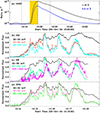 |
Fig. 1. Light curves of the solar flare on October 3, 2024. (a): Full-disk light curves during 12:00–13:00 UT measured by GOES in wavelengths of 1–8 Å (black) and 0.5–4 Å (blue). The vertical lines mark the start, peak, and stop times of the X9.0 flare. (b): Light curves from 12:13:30 UT to 12:18:50 UT measured by ASO-S/HXI in the energy range of 20–50 keV (black), 50–80 keV (tomato), and 80–300 keV (cyan). (c): Light curves between 12:13:30 UT and 12:18:50 UT recorded by KW in channels of 20–80 keV (black), 80–300 keV (spring green), and 300–1200 keV (magenta). (c): Light curves between 12:13:30 UT and 12:18:50 UT observed by STIX in channels of 20–50 keV (black), 50–80 keV (hot pink), and 80–150 keV (green). |
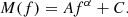
In order to identify the shorter period, a fast Fourier transform (FFT) was applied for the raw light curves with the Lomb-Scargle periodogram method (Scargle 1982), and the Fourier power spectral density (PSD) was obtained. Then, the Bayesian-based Markov chain Monte Carlo (MCMC) approach was utilized to fit the PSD with a simple model (M) that consists of a power law distribution and a constant (C) term (cf. Liang et al. 2020; Anfinogentov et al. 2021; Guo et al. 2023; Shi et al. 2023; Inglis & Hayes 2024), as is shown in Eq. (1):
Here, f denotes to the Fourier frequency, A is the amplitude, and α is the power law index. The MCMC fit results for the observational data were determined by this simple model.
Figure 2 presents the Fourier PSDs and their MCMC fit results in high-energy channels measured by HXI and KW. We note that several quasi-periods exceed the 95% confidence level in both HXRs and γ-ray continuum emissions, including the large- and small-amplitude QPPs, which correspond to the longer periods that are bigger than 10 s and the shorter period at about 1 s. On the other hand, one quasi-period at about 1 s is above the 99% confidence level, confirming that the short-period QPP really exists in HXRs and the γ-ray continuum, as is indicated by the hot pink arrow. It should be pointed out that the 3-s period in KW fluxes is attributed to the Wind’s rotation, resulting in millisecond timescales as dips in the light curves at a period of 3 s (cf. Lysenko et al. 2022).
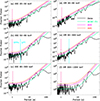 |
Fig. 2. Fourier PSDs and their MCMC fit results in log-log space. The spring green line in each panel indicates the MCMC fit for the observational data (black), the magenta, and tomato lines represent the confidence levels at 95% and 99%, respectively. The hot pink arrow outlines the interested period above the 99% confidence level. The vertical cyan line divides the spectrum into SPPs and LPT components. |
To look closely at the short-period QPP, the wavelet analysis method with a mother function of “Morlet” (Torrence & Compo 1998) was applied to the detrended time series that contains the short-period pulsations (SPPs). Using the FFT method with a Gaussian filter function (Li et al. 2017; Ning 2017; Shi et al. 2023), the raw light curve in each channel was decomposed into two components: the long-period trend (LPT) and the SPPs. Here, we used a time threshold of 3 s to distinguish the two components, as is indicated by the vertical cyan line in Figure 2. This time threshold can separate the LPT and SPP components well, because both the longer (i.e., > 10 s) and shorter periods (∼1 s) are far away from it.
Figure 3 shows the wavelet analysis results in HXR channels of HXI 50–80 keV (a1–a4) and KW 80–300 keV (b1–b4). Panels (a1) and (b1) show the normalized time series of the LPT component with the FFT filter method, and they have been normalized by their maximum intensities. They both reveal QPP signals at longer periods; that is, > 10 s. Thus, the LPT component could also be regarded as the strong background. Panels (a2) and (b2) draw the time series of SPP components. They both show the QPP patterns at a shorter period. The modulation depth of the short-period QPP, which is defined as the ratio between the SPP component and the maximum intensity of the LPT component, is much less than 10% at both HXI 50–80 keV and KW 80–300 keV. The averaged modulation depth for the short-period QPP is estimated to about 5%. Figure 3(a3)–(b4) show the wavelet power spectra and Global wavelet power spectra for the SPP component. They are dominated by a bulk of power spectra inside the 99% significance level, and all these power spectra are centered at about 1 s, which is consistent with the FFT power spectra. Moreover, the 1-s period tends to appear in the peaks of the LPT component during the flare impulsive phase; that is, from about 12:14 UT to 12:18 UT. Lastly, we present the cross-correlation analysis between the QPP patterns detected in different instruments, ASO-S/HXI and KW, in Figure A.1. The linear Pearson correlation coefficient has a maximum value of about 0.46, which occurs at the time lag of zero, as is marked by the vertical line. The correlation analysis indicates that there are not phase shifts between the QPP signals.
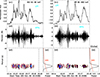 |
Fig. 3. Morlet wavelet analysis results. (a1–b2): Long-period trend (LPT) and SPPs derived from raw light curves with the FFT filter method. They have been normalized by the maximum value of the LPT component. (a3 and b3): Morlet wavelet power spectra. (a4 and b4) Global wavelet power spectra. The tomato contours and lines indicate the significance level of 99%. |
Figure 4 presents the spatial structure of the QPP pattern in multiple wavebands during the X9.0 flare. Panels (a) and (b) show the HXR maps in the energy range of 50–80 keV, and the color contours represent HXR radiation in other energy ranges. In this study, the HXR map from HXI was reconstructed by the HXI_CLEAN algorithm with a pixel scale of 2″. The HXR map from STIX was reconstructed from the expectation-maximization algorithm in the STIX Aspect System (Warmuth et al. 2020). Utilizing the Solar-MACH (Gieseler et al. 2023), panel (c) plots the spatial location of STIX and its connection with the Sun and Earth at 12:15 UT on October 3, 2024. In this event, STIX’s in situ measurements, 84.9 degrees east of the Sun-Earth line at 0.299 AU, provided a unique vantage point, along with the Earth measurements at 1 AU. Both HXI and STIX maps show two main HXR sources in the energy range of 50–300 keV or 50–150 keV, which could be considered as conjugate points that are connected by hot flare loops, as is indicated by the X-ray emission at HXI 20–50 keV (green contours). Assuming that the flare loop has a semicircular profile (cf. Tian et al. 2016; Li & Chen 2022), the flare loop length (L) can be estimated by the distance between the conjugate points, which is roughly 50 Mm. The minor radius (r) of the flare loop can be estimated by the conjugate points when assuming a circular shape for the flare loop, and it is about 2.5 Mm.
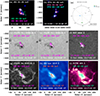 |
Fig. 4. Multiwavelength images during the X9.0 flare. (a and b): HXR maps restructured from the HXI and STIX observational data. (c) Sketch plot of the spatial location of STIX and its connection with the Sun and Earth at 12:15 UT on October 3, 2024. (d–f) White-light sub-maps measured by CHASE Fe I and WST 3600 Å. The magenta arrow indicates the movement direction of HXR sources. (g and h): Hα and Lyα images observed by CHASE and SDI. (i): The EUV snapshot captured by SUTRI at 465 Å. The contour levels are set at 10%, 50%, and 90%, respectively. |
Figure 4(d)–(f) show the white-light images measured by CHASE Fe I and ASO-S/WST 3600 Å at three times, and the overlaid contours are HXR radiation at HXI 80–300 keV. Here, the running-difference images from ASO-S/WST 3600 Å highlight the white-light emission. The three images reveal two bright patches at the edge of a sunspot group, suggesting that the X9.0 flare is a white-light flare. Moreover, the white-light brightening area matches the HXR radiation sources, indicating that the white-light emission is strongly associated with the nonthermal radiation. The HXR sources move significantly toward the southwest, as is indicated by the magenta arrow in panel (f). The displacement (D) of these two motions can be determined by the distance between the brightness centers of two adjacent footpoints, which are roughly 24 Mm and 16 Mm, respectively. Panels (g) and (h) present the Hα and Lyα images observed by CHASE and ASO-S/LST, respectively. The flare radiation in wavebands of Hα and Lyα is mainly from the upper chromosphere and low transition region on the Sun. Two strong ribbon-like features that match double HXR sources (magenta contours) can be clearly seen in the Hα and Lyα images, suggesting that the two strong ribbon-like features are double ribbons of the flare. On the other hand, a slender and elongated ribbon-like structure can also be seen in Hα and Lyα images, and it appears to have a semicircular shape. It is much weaker than the double ribbons, and it is not covered by the HXR emission. Figure 4(i) shows the EUV image captured by SUTRI at 465 Å, which is mainly formed in the upper transition region or the low corona. We can find that a bright loop-like structure appears in the EUV image, and it connects the double ribbons in Hα and Lyα images. A faint semicircular structure can also be seen in the SUTRI 465 Å image, which overlaps with the slender and elongated ribbon in the upper chromosphere or the low transition region.
4. Discussions
We systematically analyzed an X9.0 flare that was simultaneously observed on October 3, 2024, by ASO-S/HXI, KW, STIX, SUTRI, CHASE, and ASO-S/LST in wavebands of HXR, γ-ray continuum, EUV, Lyα, Hα, and white light. The X9.0 flare shows significant enhancements in wavebands of WST 3600 Å and CHASE Fe I 6569.22 Å, indicating a white-light flare. The HXI and KW light curves in the high-cadence burst mode provide us with an opportunity to investigate the short-period QPP in the energy range of HXRs and γ-ray continuum. Using the FFT method with a Bayesian-based MCMC approach (Anfinogentov et al. 2021; Guo et al. 2023; Shi et al. 2023), a quasi-period centered at about 1 s was simultaneously identified in channels of HXI 20–50 keV, 50–80 keV, and 80–300 keV, and KW 20–80 keV, 80–300 keV, and 300–1200 keV. The shorter period was also determined by the wavelet analysis method, and it appears to enhance during the impulsive phase of the X9.0 flare, especially in the HXR pulse time. The modulation depth of the short-period QPP, which was determined by the ratio between the SPPs and its LPT, was estimated to about 5% in average, suggesting that the 1-s period is a weak QPP signal. This is different from that of the long-period QPPs in HXRs and γ-rays, which often have a large modulation depth (e.g., Nakariakov et al. 2010; Li & Chen 2022; Li et al. 2024c).
The flare QPPs at the very short period, ≪1 s, are frequently observed in wavebands of radio and microwave emissions (Tan et al. 2010; Yu & Chen 2019; Karlický et al. 2024), which is attributed to the higher time resolution and the higher signal-to-noise ratio of solar radio telescopes. On the contrary, the flare QPPs in the high-energy range of HXRs and γ-rays are often identified to have a characteristic period that exceeds 4 s (e,g., Parks & Winckler 1969; Nakariakov et al. 2010; Li & Chen 2022; Collier et al. 2023; Inglis & Hayes 2024), possibly due to the observational limitation; that is, the typical signal-to-noise ratio for the HXR instrument is lower. By using the Fermi/GBM data in the burst mode, a solar flare was found to show the periodicity with a frequency of 1.7 ± 0.1 Hz (cf. Knuth & Glesener 2020), demonstrating the presence of shorter periods in the HXR channel. On the other hand, a statistical study based on the Fermi/GBM data (e.g., Inglis & Hayes 2024) suggests that the short-period QPPs at HXRs are not widespread, although they identified a few shorter periods at the timescale of about 1–4 s, similar to our results. In our case, the shorter period centered at about 1 s is also detected in the γ-ray continuum, and the QPP sources are localized by using the HXI and STIX data in two different views, which can make us explore its generation mechanism.
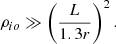
The generation mechanism of flare QPPs is still an open issue (Zimovets et al. 2021; Inglis et al. 2023). Here, we discussed the possible generation mechanism of the short-period QPP. The flare QPPs are often associated with the MHD wave. In our case, the phase speed (cP) can be estimated from the loop length (L) and the period (P), such as cP = 2L/P ≈ 1.0 × 10⁵ km s−1. The phase speed is much faster than the sound and Alfvén velocities of local plasmas. Therefore, the short-period at about 1 s might be modulated by a fast-mode wave, such as the global sausage wave. The fast kink wave is impossible, because it is essentially compressive, but it becomes “weakly compressive” or “almost incompressive” in the long-wavelength limit. On the other hand, the global sausage wave in the solar corona requires that the plasma loop must be sufficient thick and dense (Nakariakov et al. 2003); that is, the density ratio, ρio, inside and outside the flare loop should be satisfied with Eq. (2):
In our case, the density ratio is at least 237, if the shorter period is modulated by the global sausage wave. Such a ratio is much larger than the one detected in flare loops (e.g., Tian et al. 2016). So, it is difficult for the short-period to be modulated by the global sausage wave. We note that the flare footpoints evidently moved, indicating that the flare loop also moved. Thus, the lateral separations (D) of the flare loop with the variation of time can be estimated to about 24 Mm and 16 Mm, respectively. The time differences (τ) were determined by the center times in Figure 4(d)–(f), which are 76 s and 27 s. At last, the Alfvén speed (vA) should be of the order (Emslie 1981):

Here, the Alfvén speed is estimated to about 300–600 km s−1, which agrees with the previous result (Emslie 1981). Therefore, the short-period QPP can be explained by the interacting loop model presented by Emslie (1981). In this model, the small pulsations at short periods are regarded as the successive activations of a series of hot plasma loops. That is, the unstable hot loop induces a HXR pulse and then leads to the lateral expansion of magnetic lines to the nearby plasma loop, resulting in the instability and disturbance of the neighboring loop. In this process, the nonthermal electrons can be rapidly accelerated, and such a process will continue to occur from one hot loop to the neighboring loop, generating the successive and repeated HXR pulsations during the X9.0 flare (cf. Zhao et al. 2023). It should be pointed out that the interaction of different hot loops was not detected, mainly due to the observational limitation; that is, the insufficient spatial resolution and the low signal-to-noise ratio. Previous studies have suggested that the flare loop essentially consists of a number of fine-scale hot plasma loops, and they are usually regarded as a loop system (e.g., Tian et al. 2016; Li et al. 2023), which may be attributed to the diffuse nature of the EUV/SXR radiation. In a word, the interacting loop model can easily be used to explain the short-period QPP.
5. Summary
Combining the observational data measured by ASO-S/HXI, KW, STIX, CHASE, SUTRI, and GOES, we investigated the short-period QPP during a white-light flare. Our main conclusions are summarized as follows:
(1) The SPPs are simultaneously seen in the high-energy range of HXRs and the γ-ray continuum. Using the FFT and the wavelet analysis method, the quasi-period was measured to be about 1 s.
(2) The modulation depth, which was determined by the ratio between the SPPs and its LPT, was estimated to be about 5% on average, indicating a weak QPP signal.
(3) The short-period QPP during the flare impulsive phase can be interpreted by the interacting loop model presented by Emslie (1981).
Acknowledgments
The author would like to thank the referee for his/her inspiring comments. This work is supported by the Strategic Priority Research Program of the Chinese Academy of Sciences, Grant No. XDB0560000, the National Key R&D Program of China 2022YFF0503002 (2022YFF0503000). We thank the teams of ASO-S/HXI, STIX, KW, CHASE, SUTRI, and GOES for their open data use policy. ASO-S mission is supported by the Strategic Priority Research Program on Space Science, the Chinese Academy of Sciences, Grant No. XDA15320000. SUTRI is a collaborative project conducted by the National Astronomical Observatories of CAS, Peking University, Tongji University, Xi’an Institute of Optics and Precision Mechanics of CAS and the Innovation Academy for Microsatellites of CAS. The CHASE mission is supported by China National Space Administration (CNSA). The STIX instrument is an international collaboration between Switzerland, Poland, France, Czech Republic, Germany, Austria, Ireland, and Italy.
References
- Anfinogentov, S. A., Nakariakov, V. M., Pascoe, D. J., et al. 2021, ApJS, 252, 11 [NASA ADS] [CrossRef] [Google Scholar]
- Bai, X., Tian, H., Deng, Y., et al. 2023, Res. Astron. Astrophys., 23, 065014 [CrossRef] [Google Scholar]
- Brosius, J. W., & Inglis, A. R. 2018, ApJ, 867, 85 [NASA ADS] [CrossRef] [Google Scholar]
- Carley, E. P., Hayes, L. A., Murray, S. A., et al. 2019, Nat. Commun., 10, 2276 [NASA ADS] [CrossRef] [Google Scholar]
- Clarke, B. P., Hayes, L. A., Gallagher, P. T., et al. 2021, ApJ, 910, 123 [CrossRef] [Google Scholar]
- Collier, H., Hayes, L. A., Battaglia, A. F., et al. 2023, A&A, 671, A79 [NASA ADS] [CrossRef] [EDP Sciences] [Google Scholar]
- Dominique, M., Zhukov, A. N., Dolla, L., et al. 2018, Sol. Phys., 293, 61 [NASA ADS] [CrossRef] [Google Scholar]
- Emslie, A. G. 1981, ApJ, 22, 41 [Google Scholar]
- Feng, L., Li, H., Chen, B., et al. 2019, Res. Astron. Astrophys., 19, 162 [CrossRef] [Google Scholar]
- Gan, W.-Q., Zhu, C., Deng, Y.-Y., et al. 2019, Res. Astron. Astrophys., 19, 156 [Google Scholar]
- Gieseler, J., Dresing, N., Palmroos, C., et al. 2023, Front. Astron. Space Sci., 9, 384 [NASA ADS] [CrossRef] [Google Scholar]
- Guo, Y., Liang, B., Feng, S., et al. 2023, ApJ, 944, 16 [NASA ADS] [CrossRef] [Google Scholar]
- Hayes, L. A., Inglis, A. R., Christe, S., et al. 2020, ApJ, 895, 50 [NASA ADS] [CrossRef] [Google Scholar]
- Huang, J., Tan, B., Zhang, Y., et al. 2024, ApJ, 965, 137 [NASA ADS] [CrossRef] [Google Scholar]
- Inglis, A. R., & Hayes, L. A. 2024, ApJ, 971, 29 [NASA ADS] [CrossRef] [Google Scholar]
- Inglis, A., Hayes, L., Guidoni, S., et al. 2023, BAAS, 55, 181 [NASA ADS] [Google Scholar]
- Karlický, M., DudÃk, J., & Rybák, J. 2024, Sol. Phys., 299, 113 [CrossRef] [Google Scholar]
- Kashapova, L. K., Kolotkov, D. Y., Kupriyanova, E. G., et al. 2021, Sol. Phys., 296, 185 [NASA ADS] [CrossRef] [Google Scholar]
- Knuth, T., & Glesener, L. 2020, ApJ, 903, 63 [NASA ADS] [CrossRef] [Google Scholar]
- Krucker, S., Hurford, G. J., Grimm, O., et al. 2020, A&A, 642, A15 [NASA ADS] [CrossRef] [EDP Sciences] [Google Scholar]
- Li, D. 2022, Sci. China E Technol. Sci., 65, 139 [CrossRef] [Google Scholar]
- Li, D., & Chen, W. 2022, ApJ, 931, L28 [CrossRef] [Google Scholar]
- Li, D., Ning, Z. J., & Zhang, Q. M. 2015, ApJ, 807, 72 [NASA ADS] [CrossRef] [Google Scholar]
- Li, D., Zhang, Q. M., Huang, Y., et al. 2017, A&A, 597, L4 [NASA ADS] [CrossRef] [EDP Sciences] [Google Scholar]
- Li, C., Fang, C., Li, Z., et al. 2019, Res. Astron. Astrophys., 19, 165 [CrossRef] [Google Scholar]
- Li, D., Feng, S., Su, W., et al. 2020, A&A, 639, L5 [NASA ADS] [CrossRef] [EDP Sciences] [Google Scholar]
- Li, D., Ge, M., Dominique, M., et al. 2021, ApJ, 921, 179 [NASA ADS] [CrossRef] [Google Scholar]
- Li, D., Bai, X., Tian, H., et al. 2023, A&A, 675, A169 [NASA ADS] [CrossRef] [EDP Sciences] [Google Scholar]
- Li, D., Li, J., Shen, J., et al. 2024a, A&A, 690, A39 [NASA ADS] [CrossRef] [EDP Sciences] [Google Scholar]
- Li, D., Wang, J., & Huang, Y. 2024b, ApJ, 972, L2 [NASA ADS] [CrossRef] [Google Scholar]
- Li, D., Hong, Z., Hou, Z., et al. 2024c, ApJ, 970, 77 [NASA ADS] [CrossRef] [Google Scholar]
- Liang, B., Meng, Y., Feng, S., et al. 2020, Ap&SS, 365, 40 [Google Scholar]
- Lysenko, A. L., Ulanov, M. V., Kuznetsov, A. A., et al. 2022, ApJS, 262, 32 [NASA ADS] [CrossRef] [Google Scholar]
- McLaughlin, J. A., Nakariakov, V. M., Dominique, M., et al. 2018, Space Sci. Rev., 214, 45 [Google Scholar]
- Nakariakov, V. M., Melnikov, V. F., & Reznikova, V. E. 2003, A&A, 412, L7 [NASA ADS] [CrossRef] [EDP Sciences] [Google Scholar]
- Nakariakov, V. M., Foullon, C., Myagkova, I. N., et al. 2010, ApJ, 708, L47 [Google Scholar]
- Nakariakov, V. M., Kolotkov, D. Y., Kupriyanova, E. G., et al. 2019, Plasma Phys. Controll. Fusion, 61, 014024 [CrossRef] [Google Scholar]
- Ning, Z. 2017, Sol. Phys., 292, 11 [Google Scholar]
- Parks, G. K., & Winckler, J. R. 1969, ApJ, 155, L117 [Google Scholar]
- Scargle, J. D. 1982, ApJ, 263, 835 [Google Scholar]
- Shen, Y., Yao, S., Tang, Z., et al. 2022, A&A, 665, A51 [NASA ADS] [CrossRef] [EDP Sciences] [Google Scholar]
- Shi, F., Li, D., Ning, Z., et al. 2023, ApJ, 958, 39 [NASA ADS] [CrossRef] [Google Scholar]
- Su, Y., Liu, W., Li, Y.-P., et al. 2019, Res. Astron. Astrophys., 19, 163 [CrossRef] [Google Scholar]
- Tan, B., & Tan, C. 2012, ApJ, 749, 28 [NASA ADS] [CrossRef] [Google Scholar]
- Tan, B., Zhang, Y., Tan, C., et al. 2010, ApJ, 723, 25 [Google Scholar]
- Tan, B., Yu, Z., Huang, J., et al. 2016, ApJ, 833, 206 [Google Scholar]
- Tian, H. 2017, Res. Astron. Astrophys., 17, 110 [CrossRef] [Google Scholar]
- Tian, H., Young, P. R., Reeves, K. K., et al. 2016, ApJ, 823, L16 [Google Scholar]
- Torrence, C., & Compo, G. P. 1998, BAMS, 79, 61 [NASA ADS] [CrossRef] [Google Scholar]
- Warmuth, A., Önel, H., Mann, G., et al. 2020, Sol. Phys., 295, 90 [NASA ADS] [CrossRef] [Google Scholar]
- Yu, S., & Chen, B. 2019, ApJ, 872, 71 [Google Scholar]
- Yuan, D., Feng, S., Li, D., et al. 2019, ApJ, 886, L25 [Google Scholar]
- Zhao, H.-S., Li, D., Xiong, S.-L., et al. 2023, Sci. China: Phys. Mech. Astron., 66, 259611 [NASA ADS] [CrossRef] [Google Scholar]
- Zhou, X., Shen, Y., Yuan, D., et al. 2024, Nat. Commun., 15, 3281 [NASA ADS] [CrossRef] [Google Scholar]
- Zimovets, I. V., McLaughlin, J. A., Srivastava, A. K., et al. 2021, Space Sci. Rev., 217, 66 [NASA ADS] [CrossRef] [Google Scholar]
- Zimovets, I. V., Nechaeva, A. B., Sharykin, I. N., et al. 2022, Geomagn. Aeron., 62, 356 [NASA ADS] [CrossRef] [Google Scholar]
Appendix A: Cross-correlation analysis
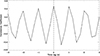 |
Fig. A.1. Cross-correlation analysis between the QPP patterns detected in two different instruments, i.e., HXI and KW. The time series represents the cross-correlation coefficients as a function of the time lag. The vertical line marks the maximum coefficient. |
All Figures
|
Fig. 1. Light curves of the solar flare on October 3, 2024. (a): Full-disk light curves during 12:00–13:00 UT measured by GOES in wavelengths of 1–8 Å (black) and 0.5–4 Å (blue). The vertical lines mark the start, peak, and stop times of the X9.0 flare. (b): Light curves from 12:13:30 UT to 12:18:50 UT measured by ASO-S/HXI in the energy range of 20–50 keV (black), 50–80 keV (tomato), and 80–300 keV (cyan). (c): Light curves between 12:13:30 UT and 12:18:50 UT recorded by KW in channels of 20–80 keV (black), 80–300 keV (spring green), and 300–1200 keV (magenta). (c): Light curves between 12:13:30 UT and 12:18:50 UT observed by STIX in channels of 20–50 keV (black), 50–80 keV (hot pink), and 80–150 keV (green). |
| In the text | |
|
Fig. 2. Fourier PSDs and their MCMC fit results in log-log space. The spring green line in each panel indicates the MCMC fit for the observational data (black), the magenta, and tomato lines represent the confidence levels at 95% and 99%, respectively. The hot pink arrow outlines the interested period above the 99% confidence level. The vertical cyan line divides the spectrum into SPPs and LPT components. |
| In the text | |
|
Fig. 3. Morlet wavelet analysis results. (a1–b2): Long-period trend (LPT) and SPPs derived from raw light curves with the FFT filter method. They have been normalized by the maximum value of the LPT component. (a3 and b3): Morlet wavelet power spectra. (a4 and b4) Global wavelet power spectra. The tomato contours and lines indicate the significance level of 99%. |
| In the text | |
|
Fig. 4. Multiwavelength images during the X9.0 flare. (a and b): HXR maps restructured from the HXI and STIX observational data. (c) Sketch plot of the spatial location of STIX and its connection with the Sun and Earth at 12:15 UT on October 3, 2024. (d–f) White-light sub-maps measured by CHASE Fe I and WST 3600 Å. The magenta arrow indicates the movement direction of HXR sources. (g and h): Hα and Lyα images observed by CHASE and SDI. (i): The EUV snapshot captured by SUTRI at 465 Å. The contour levels are set at 10%, 50%, and 90%, respectively. |
| In the text | |
|
Fig. A.1. Cross-correlation analysis between the QPP patterns detected in two different instruments, i.e., HXI and KW. The time series represents the cross-correlation coefficients as a function of the time lag. The vertical line marks the maximum coefficient. |
| In the text | |
Current usage metrics show cumulative count of Article Views (full-text article views including HTML views, PDF and ePub downloads, according to the available data) and Abstracts Views on Vision4Press platform.
Data correspond to usage on the plateform after 2015. The current usage metrics is available 48-96 hours after online publication and is updated daily on week days.
Initial download of the metrics may take a while.