| Issue |
A&A
Volume 690, October 2024
|
|
|---|---|---|
| Article Number | A39 | |
| Number of page(s) | 7 | |
| Section | The Sun and the Heliosphere | |
| DOI | https://doi.org/10.1051/0004-6361/202450622 | |
| Published online | 27 September 2024 | |
Long-period energy releases during a C2.8 flare
1
Key Laboratory of Dark Matter and Space Astronomy, Purple Mountain Observatory, Chinese Academy of Sciences, Nanjing 210023, PR China
2
State Key Laboratory of Space Weather, Chinese Academy of Sciences Beijing 100190, PR China
3
, Xinjiang Astronomical Observatory, Chinese Academy of Sciences, Urumqi 830011, PR China
Received:
6
May
2024
Accepted:
24
July
2024
Abstract
Context. The study of quasi-periodic pulsations (QPPs) is a key diagnostic of intermittent or periodic energy releases during solar flares.
Aims. We investigated the intermittent energy-releasing processes by analyzing the long-period pulsations during a C2.8 flare on 2023 June 3.
Methods. The solar flare was simultaneously observed by the solar X-ray detector on board the Macau Science Satellite-1B, the Geostationary Operational Environmental Satellite, the Chinese Hα Solar Explorer, the Expanded Owens Valley Solar Array, the Atmospheric Imaging Assembly, and the Extreme Ultraviolet Variability Experiment for the Solar Dynamics Observatory.
Results. The C2.8 flare shows three successive and repetitive pulsations in soft X-ray (SXR) and high-temperature extreme ultraviolet (EUV) emissions, which may imply three episodes of energy releases during the solar flare. The QPP period is estimated to be as long as ∼7.5 minutes. EUV imaging observations suggest that these three pulsations come from the same flare area dominated by the hot loop system. Conversely, the flare radiation in wavelengths of radio/microwave, low-temperature EUV, ultraviolet (UV), and Hα only reveals the first pulsation, which may be associated with nonthermal electrons accelerated by magnetic reconnection. The other two pulsations in wavelengths of SXR and high-temperature EUV might be caused by the loop-loop interaction.
Conclusions. Our observations indicate that the three episodes of energy releases during the C2.8 flare are triggered by different mechanisms, namely the accelerated electron via magnetic reconnection, and the loop-loop interaction in a complicated magnetic configuration.
Key words: Sun: flares / Sun: radio radiation / Sun: UV radiation / Sun: X-rays / gamma rays
Corresponding author; This email address is being protected from spambots. You need JavaScript enabled to view it. .
© The Authors 2024
 Open Access article, published by EDP Sciences, under the terms of the Creative Commons Attribution License (https://creativecommons.org/licenses/by/4.0), which permits unrestricted use, distribution, and reproduction in any medium, provided the original work is properly cited.
This article is published in open access under the Subscribe to Open model. This email address is being protected from spambots. You need JavaScript enabled to view it. to support open access publication.
1. Introduction
A solar flare is an explosive and impulsive energy-releasing phenomenon via the well-known magnetic reconnection, which can be detected in multi-height solar atmospheres (Benz 2017). The released energy is mainly converted from the free magnetic energy that is stored in the nonpotential magnetic field, which overlaps the current-carrying field and is dominated by a complex magnetic geometry (Jiang et al. 2021; Yan et al. 2022; McKevitt et al. 2024). As described in the classical two-dimensional (2D) flare model (Priest & Forbes 2002), the free magnetic energy may release violently and suddenly in the solar coronal active region, which can rapidly heat thermal plasmas to the temperature of several million Kelvin (MK), and they can quickly accelerate nonthermal particles to a high energy range of dozens of keV to GeV (e.g., Warmuth & Mann 2016; Li et al. 2021a). In the imaging observation for a typical solar flare, double footpoints are seen in hard X-ray (HXR) or microwave emissions, and a loop-like structure that connects double footpoints appears in soft X-ray (SXR) and extreme ultraviolet (EUV) wavelengths, while the loop-top source might be observed in HXR or microwave channels (e.g., Masuda et al. 1994; Yan et al. 2018; Li et al. 2023a). Meanwhile, two ribbon-like features can be found in wavelengths of ultraviolet (UV), white light (WL), or Hα (Li et al. 2017; Tian 2017). This is called a two-ribbon flare, which is the most common flare and matches the standard 2D reconnection model (Priest & Forbes 2002). If the magnetic configuration becomes more complicated, then the three-ribbon flare (e.g., Wang et al. 2014; Zimovets et al. 2021a) or circular-ribbon flare (e.g., Masson et al. 2009; Ning et al. 2022) are observed on the Sun, which may be associated with various 3D magnetic configurations (Janvier et al. 2015; Zhang 2024).
A solar flare is commonly powered by the release process of free magnetic energy (Priest & Forbes 2002; Shen et al. 2023). Such an energy release is often characterized by repeated and successive processes, which is manifested as quasi-periodic pulsations (QPPs) in the time series of flare radiation (Nakariakov et al. 2019; Zimovets et al. 2021b, and references therein). The typical QPP often has at least three successive and complete peaks, namely three QPP cycles. If there are only one or two peaks, it might just be a coincidence; that is, the similar time interval between successive peaks occurred by chance (e.g., McLaughlin et al. 2018; Li et al. 2022a). A QPP event usually carries the abundant information of time characteristics and plasma features in the flare source, and thus it plays a crucial role in diagnosing the coronal parameter of the Sun or remote solar-like stars (Yuan et al. 2019; Kolotkov et al. 2021; Li et al. 2021b; Inglis et al. 2023). The flare QPPs were first reported by Parks & Winckler (1969) in temporal-intensity profiles at X-ray and radio emissions. To date, they have been observed in a broad wavelength range of electromagnetic radiation: radio/microwave, Hα, Lyα, UV/EUV, SXR/HXR, and gamma-rays (e.g., Brosius & Daw 2015; Nakariakov et al. 2018; Chen et al. 2019; Hayes et al. 2019; Li et al. 2020a,b; Milligan et al. 2020; Hong et al. 2021; Li 2022; Motyk et al. 2023). Their periods were measured from subseconds through seconds to several minutes (e.g., Tian et al. 2008; Samanta et al. 2021; Shen et al. 2022; Zimovets et al. 2022; Li et al. 2023b; Collier et al. 2023; Mehta et al. 2023; Zhao et al. 2023; Zhou et al. 2024). It seems that the detected periods were always dependent on the studied wavebands or flare phases, indicating that flare QPPs belonging to different categories may be generated by various mechanisms or models (Kupriyanova et al. 2020). There was not a single mechanism that can fully interpret the presence of all flare QPPs because there was not enough observational data to distinguish between the various mechanisms (Inglis et al. 2023). The flare QPPs at periods of subseconds were always measured in radio and microwave emissions, which were usually produced by dynamic interactions between energetic ions and electromagnetic waves that were trapped in complex magnetic fields (Aschwanden 1987; Tan & Tan 2012). The flare QPPs at long periods of seconds or minutes can be observed in nearly all the wavebands such as radio, Hα, Lα, UV/EUV, SXR/HXR, and they are commonly associated with the magnetohydrodynamic (MHD) waves in various modes (see Nakariakov & Kolotkov 2020). Moreover, the flare QPPs detected in wavelengths of HXR and microwave emissions during the impulsive phase were frequently interpreted in terms of nonthermal electrons periodically accelerated by repetitive magnetic reconnections (Farhang et al. 2022; Li & Chen 2022; Karampelas et al. 2023; Karlický & Rybák 2023; Corchado Albelo et al. 2024).
One key signature of the flare energy-releasing process is impulsive, repetitive, or intermittent, which may be strongly dependent on the time profiles on timescales of minutes, seconds, and milliseconds (cf. Inglis et al. 2023). Such signatures of energy release are often associated with the flare radiation observed in multiple wavelengths that is bursty and periodic; in other words, the flare radiation is frequently modulated by a pattern of QPPs. Therefore, the study of flare QPPs is a crucial diagnostic of the intermittent energy releases on the Sun. For this article we investigated the intermittent energy releases with long periods during the C2.8 flare on 2023 June 3. The article is organized as follows: Section 2 introduces the observations and instruments, Section 3 shows the data analysis and our main results, and Section 4 presents some discussion, while a brief summary is given in Section 5.
2. Observations and Instruments
The targeted solar flare occurred in the active region of NOAA 13319. It was a C2.8 class flare, that started at ∼21:40 UT on 2023 June 3, peaked at ∼21:47 UT, and stopped at about ∼22:10 UT1. The C2.8 flare was simultaneously measured by multiple space- and ground-based instruments: the solar X-ray detector (SXD) on board the Macau Science Satellite-1B (MSS-1B; Shi et al. 2023); the Geostationary Operational Environmental Satellite (GOES; Chamberlin et al. 2009); the Large-Yield RAdiometer (LYRA; Dominique et al. 2013) on board the PRoject for On-Board Autonomy 2 (PROBA2); the Atmospheric Imaging Assembly (AIA; Lemen et al. 2012) and the EUV SpectroPhotometer (ESP; Didkovsky et al. 2012) for the Solar Dynamics Observatory (SDO); the Chinese Hα Solar Explorer (CHASE; Li et al. 2022b); the STEREO/WAVES instrument (SWAVES; Kaiser et al. 2008); the Expanded Owens Valley Solar Array (EOVSA; Gary et al. 2011); and the e-CALLISTO radio spectrograph at NORWAY.
The Macau Science Satellite-1 (MSS-1) includes two subsatellites, named MSS-1A and MSS-1B. SXD on board MSS-1B is designed to monitor the full-disk solar spectrum in the SXR/HXR energy range of about 1−600 keV (or ∼0.02−12 Å), and thus it has two parts: the SXR detection unit (SXDU) and the HXR detection unit (HXDU). The time cadence is as high as ∼1 s. GOES records the full-disk solar irradiance in SXR 1−8 Å and 0.5−4 Å with a time cadence of 1 s, and the isothermal temperature of SXR-emitting plasma can be determined from their ratio. SDO/ESP provides the full-disk solar irradiance with a time cadence of 0.25 s, which contains one SXR and four EUV wavebands. LYRA measures the full-disk solar radiation in two far-ultraviolet (FUV) and two X-ray ultraviolet (XUV) wavebands with a time cadence of 0.05 s. SDO/AIA simultaneously measures the entire-Sun maps in seven EUV and two UV wavelengths with a spatial scale of 0.6″ via a standard pre-process. The time cadence for the EUV waveband is 12 s, and that for the UV wavelengths is 24 s. CHASE takes the spectroscopic observation of the whole Sun in passbands of Hα with a pixel scale of 1.04″, and a time cadence of about 71 s. EOVSA is a radioheliograph, and it acquires the solar dynamic spectrum in the microwave frequency of 1−18 GHz with a time cadence of roughly 1 s. The e-CALLISTO radio spectrograph at NORWAY observes the solar radio spectrum in the frequency range of ∼1.0−1.6 GHz with a time cadence of ∼0.5 s. SWAVES provides the solar radio spectrum at frequencies of about 0.0026−16.025 MHz with a time cadence of 60 s.
3. Data analysis and results
Figure 1 presents the multiwavelength observations of the targeted flare on 2023 June 3. The whole evolution of the flare can be seen in the online animation. Figure 1a shows the SXR/XUV light curves integrated over the whole Sun between 21:40 UT and 22:10 UT. The GOES flux at 1−8 Å (black) indicates a C2.8 class flare that reached its maximum at about 21:47 UT, as marked by the dashed vertical line. The C2.8 flare also reveals another two pulsations (labeled 2 and 3), which occurred at about 21:55 UT and 22:02 UT in the GOES 1−8 Å flux, respectively, following closely after the first pulsation (labeled 1). The three successive pulsations might be regarded as a flare QPP with an average period of about 7.5 minutes. These three successive pulsations can also be seen in the SXR/XUV light curves recorded by SXDU 1−10 Å, ESP 1−70 Å, and LYRA 1−200 Å, suggesting that the QPP feature is visible by all the available instruments. We also note that the longer the observed wavelengths, the later the peak times, which means that the SXR flux at ESP 1−70 Å (magenta) is clearly later than that at SXDU 1−10 Å (gold). This is because the different peak times could have to do with different responses of the instruments to the temperature of the plasma. The SXR/XUV fluxes are integrated over the entire Sun, making it difficult to determine whether these three pulsations come from the same flare area. The SDO/AIA data can spatially resolve the flare region from the whole Sun, and the local light curves in EUV wavebands are integrated over the active region, as outlined by the pink box in panel b. It can be seen that the local light curves at AIA 131 Å (cyan) and 94 Å also show three successive pulsations, confirming that they originate from the same active region. Panels b and c show AIA submaps with a field of view (FOV) of ∼100″ × 100″. The flare reveals some ribbons in the AIA 1600 Å image, as outlined by the black contours. These ribbons are connected by two groups of hot loop systems, as can be seen in the AIA 131 Å image.
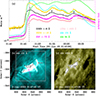 |
Fig. 1. Overview of the C2.8 flare on 2023 June 3. Panel a: Full-disk light curves recorded by GOES 1−8 Å (black), SXDU 1−10 Å (gold), ESP 1−70 Å (magenta), and LYRA 1−200 Å (pink), as well as the local fluxes measured by SDO/AIA at 131 Å (cyan) and 94 Å (green). The vertical line marks the flare peak time. Panels b and c: EUV/UV snapshots with a FOV of ∼100″ × 100″ in wavelengths of AIA 131 Å and 1600 Å. The black contours outline flare ribbons in AIA 1600 Å. The colored arrows indicate hot loop systems. The pink box marks the flare region (∼72″ × 72″) used to integrate the local flux. A movie associated to this figure is available online. |
The SXR light curves recorded by SXDU 1−10 Å and GOES 1−8 Å appear to match each other, confirming that the newly launched MSS-1B/SXD can also be applied to monitor the solar irradiance. Figure 2a shows the energy spectrum in the SXR range of 1−10 Å that was captured by MSS-1B/SXDU. In order to improve the signal-to-noise ratio, the energy spectrum was integrated over 60 s during the C2.8 flare (i.e., during 21:47−21:48 UT). It is immediately clear that the SXR energy spectrum is mainly composed of two spectral lines superposed on a strong background profile. The two spectral lines contains a group of lines of highly stripped iron (Fe) and calcium (Ca) ions (Phillips 2004). They both show Gaussian profiles, and a single Gaussian function is applied to fit, as indicated by the magenta and cyan curves, respectively. Then, their fitting peak intensities and center positions are extracted, as shown in Figures 2b and c. The black line in panel b represents the SXR flux recorded by SXDU 1−10 Å with a time cadence of 60 s. All these curves, such as the fitting peak and center of Fe and Ca, reveal three successive pulsations, similarly to what was observed in the SXR flux recorded by GOES 1−8 Å.
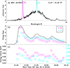 |
Fig. 2. Observational results measured from MSS-1B/SXDU. Panel a: SXR spectrum integrated over one minute during the C2.8 flare in the range 1−10 Å. The magenta and cyan curves represent the Gaussian fitting results for the Fe and Ca lines, respectively. Panels b and c: Time series of the fitting peak and center for Fe (circular) and Ca (diamond) lines. |
To investigate the origin or driver of the flare QPP that was simultaneously detected in wavelengths of SXR, high-temperature EUV, and spectral lines, Figure 3 presents more light curves during the C2.8 flare. Panel a plots the time series of isothermal temperature and SXR derivative that were derived from two GOES fluxes. Similar to what was seen in the SXR fluxes, the temperature profile also exhibits three main pulsations, suggesting that the flare QPP is sensitive to the plasma temperature. Conversely, the SXR 1−8 derivative flux only reveals clearly the first pulsation (1), the other two pulsations (2 and 3) are very weak and even invisible, which may indicate that the first pulsation is highly associated with the nonthermal electron. Panel b shows the local EUV/UV fluxes (pink box in Figure 1) in wavelengths of AIA 171 Å, 304 Å, 335 Å, and 1600 Å. They all have the first pulsation, but the other two pulsations are invisible (2) or weak (3). The AIA 335 Å flux appears to continually enhance after the first pulsation, which is absolutely different from the previous observation in SXR channels. Panel c shows the radio fluxes in frequencies of EOVSA 6.20 GHz, NORWAY 1.23 GHz, and SWAVES 1.93 MHz. We can see that they all show one pulsation at about 21:46 UT, which is consistent with the SXR derivative flux, suggesting that the electron beam is accelerated during the impulsive phase of the C2.8 flare. The context image is the radio dynamic spectrum captured by EOVSA in the high-frequency range of 1−18 GHz, and it shows a radio burst accompanied by the first pulsation, confirming the presence of accelerated electrons.
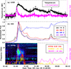 |
Fig. 3. Multiwavelength light curves during the C2.8 flare. Panel a: Full-disk light curves for the GOES temperature (black) and SXR 1−8 Å derivative (magenta). Panel b: Local fluxes in wavelengths of AIA 171 Å (black), 304 Å (red), 335 Å (blue), and 1600 Å (purple). Panel c: Radio light curves in frequencies of EOVSA 6.60 GHz (red), NORWAY 1.23 GHz (gold), and SWAVES 1.93 MHz (magenta). The context image is the radio dynamic spectrum measured by EOVSA. |
Figure 4 gives a close look at the source region of the flare QPP, showing the multiwavelength images with a small FOV of ∼72″ × 72″ at four time instances measured by SDO/AIA at 131 Å (a1–a4), 335 Å (b1–b4), and 304 Å (c1–c4), and CHASE Hα at 6562.8 Å (d1–d4). Here, the different AIA-based images are given to show the flare structure clearly, and the initial image is taken from the image captured two minutes before the flare onset. The Hα raw images are given, since the CHASE begins to observe the Sun after the flare onset and there are no pre-flare images. Panels a1, b1, and c1 show the different AIA images at the flare onset time, and they all reveal very weak radiation in the flare region. Panel d1 presents the first Hα image measured by CHASE during its observation for the C2.8 flare, and it exhibits some Hα kernels, as marked by the blue arrows. Panels a2, b2, c2, and d2 show the AIA and CHASE images during the first pulsation (1). A group of hot loop-like structures can be clearly seen in the wavelength of AIA 131 Å, which is regarded as the flare loop system, and is outlined by the magenta contour (arrow). Meanwhile, a weak loop system is also seen (marked by the red arrow). On the other hand, two strong ribbon-like features that are connected by the flare loop system (i.e., L1) appear in wavelengths of AIA 335 Å and 304 Å, and the CHASE Hα line center. Moreover, a weak kernel-like structure (indicated by a gold arrow) appears in these three images, which is connected by a weak hot loop (i.e., L2). During the second pulsation (2) of the C2.8 flare, two groups of loop-like structures are seen in the high-temperature EUV channel, as indicated by the magenta contours in panel a3. These middle- and low-temperature channels exhibits at least four kernel-like structures, but they are a bit weaker, as indicated by the green contours in panels b3, c3, and d3. Interestingly, two hot loop systems connect these four kernels, which may be regarded as flare footpoints. During the third pulsation (3) of the C2.8 flare, the two hot loop systems and their corresponding ribbons or footpoints can also be seen in EUV and Hα images, as shown in panels a4, b4, c4, and d4. All these observations suggest that the C2.8 flare shows multiple ribbons, at least four flare ribbons. Then, two regions (red rectangles) that contain two flare loop systems are separated to integrate their intensity curves.
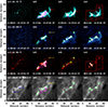 |
Fig. 4. Multiwavelength images with a FOV of ∼72″ × 72″ during the C2.8 flare. Panels a1–c4: Base different images measured by SDO/AIA at 131 Å, 335 Å, and 304 Å. Panels d1–d4: Hα images observed by CHASE. The magenta contour represents the hot plasma emission from AIA 131 Å, while the green contours are the plasma radiation from Hα. The magenta an red arrows mark the flare loops, while the blue and gold arrows outline the flare kernels. The red rectangles contain two hot loop systems (L1 and L2) at AIA 131 Å. |
Figure 5 shows the time series of the AIA intensity at two loop-dominated regions. The solid line is integrated over from the main strong loop system (L1), while the dashed line is integrated over another weak loop system (L2). Panel a presents the light curves in high-temperature EUV channels, such as AIA 131 Å and 94 Å. Similarly to what has been seen in the SXR/XUV channels, both the AIA 131 Å and 94 Å fluxes at the main strong loop system (L1) show three pronounced pulsations during the C2.8 flare, and they also appear to exhibit a decreasing trend, as indicated by the solid black and green line profiles. On the other hand, the AIA 131 Å flux at the weak loop system (L2) also have three small peaks, while the AIA 94 Å flux at L2 loop mainly shows an increasing trend. The similar monotonous growth can also be found at the weak L2 loop system in wavelengths of AIA 335 Å and 211 Å, as shown by the dashed line curves in panel b. However, such monotonic growth cannot be seen in the AIA 304 Å and 1600 Å fluxes, nor can it be seen in the Hα 6562.8 Å light curve at the L2 loop system, as indicated by the dashed line profiles in panel c. Figures 5b and c also demonstrate that the light curves at the L1 loop system only have one main pulsation (i.e., pulsation 1). Although the light curves at AIA 335 Å and 211 Å appear as two subpeaks (I and II), they are still in the time interval of pulsation 1. We also note that there is also a subpeak III during pulsation 3 at the L1 loop in almost all the observed wavelengths, but they are much weaker than the first pulsation 1, which is different from that in the AIA high-temperature channels. All these observations suggest that the three pulsations are basally from the flare area dominated by the strong loop system.
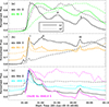 |
Fig. 5. Local light curves measured by SDO/AIA and CHASE Hα. The solid and dashed curves are integrated over the flare loop regions of L1 and L2, respectively. |
4. Discussions
Based on the multi-instrument observations, we investigated the flare QPP with a long period in wavelengths of SXR/XUV and high-temperature EUV. The flare QPP was first observed in the full-disk light curves in SXR/XUV channels of GOES 1−8 Å, SXDU 1−10 Å, ESP 1−70 Å, and LYRA 1−200 Å. There are three successive and significant pulsations with a long duration. The three pulsations in GOES 1−8 Å flux are peaked at about 21:47 UT, 21:55 UT, and 22:02 UT. The average period is about 7.5 minutes. We also note that the peak time of each pulsation occurs later with increasing detected channels, which may because the certain waveband emission might be dominated in a different time of the flare, and it is consistent with our previous observations (e.g., Li et al. 2023a). Then, the flare QPP with three successive pulsations was also detected in the local light curves that are integrated over the flare region at the high-temperature EUV wavebands of AIA 131 Å and 94 Å, indicating that the QPP feature originates from the same flare region. However, the flare QPP could not be observed in the GOES 1−8 Å derivative flux, which is regarded as the HXR flux according to the Neupert effect (e.g., Neupert 1968; Li et al. 2024a), since we could not find the available HXR light curve during the C2.8 flare. Moreover, the flare QPP was also not detected in the radio emission, at high or low frequencies, and it was not seen in the local light curves at the middle- and low-temperature AIA channels and the Hα line center. On the other hand, the light curves in these channels show one pronounced peak that corresponds to pulsation 1, suggesting that pulsation 1 may be caused by the electron beam accelerated by the magnetic reconnection, as described in the standard 2D reconnection model (Priest & Forbes 2002). Instead, the two later pulsations might be due to the interaction of some blended loops since we can find a series of hot loops in the AIA 131 Å images, which are regarded as flare loop systems, as seen in the online animation.
The flare QPP with three successive pulsations in multiple wavelengths suggests three energy-releasing processes at a long period during the C2.8 flare. We note that the three pulsations in the wavelength of AIA 94 Å appear as an increasing trend; that is, the peak intensity of pulsation 3 is obviously larger than that of pulsation 1 (Figure 1a). This feature is definitively different from that in the wavelength of AIA 131 Å, GOES 1−8 Å, and SXDU 1−10 Å, all of which show a decreasing trend. We then decomposed the whole flare region into two loop-dominated regions (L1 and L2) by using the AIA images in EUV/UV wavelengths. The strong loop-dominated region is considered the main flare region, and the light curves at AIA 131 Å and 94 Å that integrated over this main region show a very similar decreasing trend, suggesting that the strong loop-dominated region (L1) is the generated source of the flare QPP. While the weak loop-dominated region (L2) is considered the accompanying flare area, and the light curves at AIA 94 Å, 335 Å, and 211 Å that integrated over this accompanying region reveal a trend of monotonic growth. Therefore, the light curves at the middle-temperature EUV channels show an increasing trend. It should be noted that the middle-temperature channels are the EUV data in wavelengths of AIA 94 Å, 335 Å, and 211 Å, which is distinguished from the high-temperature channel at AIA 131 Å and the low-temperature channels at AIA 171 Å, 304 Å, 1600 Å, and CHASE Hα. The light curves at the low-temperature channels only show one pronounced pulsation at the strong loop-dominated region, similar to previous observations at the whole flare region in the radio emission.
The flare QPP under study is different from previous flare QPPs observed in SXR/EUV channels. Here, we reported a QPP event within a long period of about 7.5 minutes during the entire flare phases (i.e., from the impulsive phase through the main phase to the decay phase). The previous QPPs events were often observed in multiple channels of SXR, EUV, HXR, and radio/microwave during solar–stellar flares, and their periods were commonly on a timescale of seconds or minutes (e.g., Nakariakov et al. 2018; Kolotkov et al. 2021; Hong et al. 2021; Li 2022; Zimovets et al. 2022; Mehta et al. 2023; Corchado Albelo et al. 2024). Moreover, the flare QPPs were frequently related to nonthermal particles periodically accelerated by repetitive magnetic reconnections, especially when they were detected simultaneously in HXR and microwave fluxes during the impulsive phase of solar flares (e.g., Yuan et al. 2019; Karampelas et al. 2023; Li et al. 2024b). The very long-period pulsations (VLPs) with periods of ∼8−30 minutes have also been detected in wavelengths of SXR (Tan et al. 2016) and Hα (Li et al. 2020b). However, those VLPs were found before the onset of major solar flares rather than during the solar flares themselves. Therefore, these VLPs might be some recurrences of small flares before the major flare. In this case, the three pulsations were located in the same region dominated by a group of loop-like structures, which is regarded as one flare (see also the solar monitor). The flare QPPs were also reported during the entire phases of a solar flare, but they usually showed various periods in different flare phases (Hayes et al. 2019; Li et al. 2020c, 2021b; Collier et al. 2023). For instance, Hayes et al. (2019) reported the QPP with a period of ∼65 s in the impulsive phase followed by the QPP with a period of ∼150 s in the decay phase, which was also different from our case. In summary, we first reported a long-period QPP during the entire flare phase in wavelengths of SXR, XUV, and high-temperature EUV.
The QPP behavior seen in the fitting center of Fe and Ca lines mainly occurs because of the periodic variation of plasma temperatures. Using a single Gaussian function with a linear trend, we fitted the line profiles of Fe and Ca lines. Then, their fitting peak intensities and line centers were extracted, both of which show the QPP feature with a period of about 7.5 minutes. The fitting peak intensity is the peak radiation of Fe and Ca lines during the C2.8 flare. However, it was impossible to determine the Doppler shift of these two lines, although we extracted the fitting line centers. This is because we could not identify their reference line centers. Figure 6 presents the synthetic SXR spectra in the energy range of 6.2−6.9 keV, which is computed from the CHIANTI database (Del Zanna et al. 2021) for the flare condition at two temperatures: Log10T = 7.0 (a) and Log10T = 7.2 (b). We note that the line profile of Fe line is actually composed of a series of highly ionized iron ions; that is, the dominant spectral lines are varied from Fe XX to Fe XXV with increasing plasma temperature. So it is impossible to determine the line center of each spectral line, mainly due to the limitation of the spectral resolution of MSS-1B/SXDU. In our case the spectral lines are simply called the Fe line, and the periodic variation of fitting centers at the Fe line is largely caused by the periodic disturbances of the plasma temperature during the C2.8 flare. This was demonstrated by the oscillation of the isothermal temperature of SXR-emitting plasmas that were determined by two GOES SXR fluxes, as seen in Figure 3a.
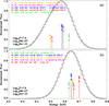 |
Fig. 6. Synthetic SXR spectra in the energy range between 6.2 keV and 6.9 keV from the CHIANTI database at plasma temperatures (Log10T) of 7.0 (a) and 7.2 (b), respectively. The colored lines mark the five strongest lines at the high-order ionized iron in the given condition. |
5. Summary
Using the spaced- and ground-based telescopes, MSS-1B/SXDU, CHASE, GOES, PROBA2/LYRA, SDO/AIA, SDO/EVE, e-CALLISTO/NORWAY, SWAVES, and EOVSA, we reported the observation of a QPP event during a four-ribbon flare on 2023 June 3. Our main results are summarized as follows:
(1) The flare QPP with an average period of about 7.5 minutes was simultaneously detected in SXR, XUV, and high-temperature EUV channels. It manifests as three pronounced pulsations in the light curves at GOES 1−8 Å, SXDU 1−10 Å, ESP 1−70 Å, LYRA 1−200 Å, AIA 131 Å, and 94 Å; it can also be seen in the time series of GOES temperature, the fitting peak, and the center of the Fe and Ca lines.
(2) The flare QPP cannot be observed in the high- and low-frequency radio emissions, and the middle- and low-temperature EUV/UV wavelengths. Only one main pulsation (1) can be found in the time series of GOES 1−8 Å derivative, EOVSA 6.60 GHz, NORWAY 1.23 GHz, and SWAVES 1.93 MHz, as well as the AIA 171 Å, 304 Å, 335 Å, and 1600 Å, and Hα 6562.8 Å. This observational fact implies that the first pulsation is highly associated with the nonthermal electron accelerated by magnetic reconnection.
(3) AIA imaging observations show that the C2.8 flares have double loop systems that connect four ribbons or kernels, and the QPP feature is mainly from the flare area characterized by a strong loop system.
(4) The QPP feature seen in time series of the fitting peak and center of the Fe and Ca lines may be due to the periodic variety of the plasma temperature, causing the ion and calcium into high-order ionizations.
(5) The flare QPP with three main pulsations suggest three energy-releasing processes. The first energy-releasing process is caused by the accelerated electron, while the later two energy-releasing processes might be due to the loop-loop interaction in the strong loop system.
Data availability
Movie is available at https://www.aanda.org
Acknowledgments
We gratefully acknowledge the referee for his or her inspiring comments. This work is funded by NSFC under grants 12250014, 12273101 12073081, the National Key R&D Program of China 2021YFA1600502 (2021YFA1600500). This work is supported by the Macao Foundation. D. Li is also supported by the Specialized Research Fund for State Key Laboratories. This work is also supported by the Strategic Priority Research Program of the Chinese Academy of Sciences, Grant No. XDB0560000. We thank the teams of MSS-1B, CHASE, GOES, PROBA2, SDO, e-CALLISTO, SWAVES, and EOVSA for their open data use policy. The authors would also like to thank Drs. Chuan Li and Ye Qiu for their discussions about the CHASE data, and Dr. Sijie Yu for discussing the EOVSA data. The CHASE mission is supported by China National Space Administration (CNSA).
References
- Aschwanden, M. J. 1987, Sol. Phys., 111, 113 [NASA ADS] [CrossRef] [Google Scholar]
- Benz, A. O. 2017, Liv. Rev. Sol. Phys., 14, 2 [Google Scholar]
- Brosius, J. W., & Daw, A. N. 2015, ApJ, 810, 45 [NASA ADS] [CrossRef] [Google Scholar]
- Chen, X., Yan, Y., Tan, B., et al. 2019, ApJ, 878, 78 [NASA ADS] [CrossRef] [Google Scholar]
- Chamberlin, P. C., Woods, T. N., Eparvier, F. G., et al. 2009, Proc. SPIE, 7438, 743802 [CrossRef] [Google Scholar]
- Collier, H., Hayes, L. A., Battaglia, A. F., et al. 2023, A&A, 671, A79 [NASA ADS] [CrossRef] [EDP Sciences] [Google Scholar]
- Corchado Albelo, M. F., Kazachenko, M. D., & Lynch, B. J. 2024, ApJ, 965, 16 [NASA ADS] [CrossRef] [Google Scholar]
- Didkovsky, L., Judge, D., Wieman, S., et al. 2012, Sol. Phys., 275, 179 [NASA ADS] [CrossRef] [Google Scholar]
- Del Zanna, G., Dere, K. P., Young, P. R., et al. 2021, ApJ, 909, 38 [NASA ADS] [CrossRef] [Google Scholar]
- Dominique, M., Hochedez, J.-F., Schmutz, W., et al. 2013, Sol. Phys., 286, 21 [NASA ADS] [CrossRef] [Google Scholar]
- Farhang, N., Shahbazi, F., & Safari, H. 2022, ApJ, 936, 87 [NASA ADS] [CrossRef] [Google Scholar]
- Gary, D. E., Hurford, G. J., Nita, G. M., et al. 2011, AAS/Solar Physics Division Abstracts, 42, 1.02 [NASA ADS] [Google Scholar]
- Hayes, L. A., Gallagher, P. T., Dennis, B. R., et al. 2019, ApJ, 875, 33 [Google Scholar]
- Hong, Z., Li, D., Zhang, M., et al. 2021, Sol. Phys., 296, 171 [NASA ADS] [CrossRef] [Google Scholar]
- Inglis, A., Hayes, L., Guidoni, S., et al. 2023, BAAS, 55, 181 [NASA ADS] [Google Scholar]
- Janvier, M., Aulanier, G., & Démoulin, P. 2015, Sol. Phys., 290, 3425 [Google Scholar]
- Jiang, C., Feng, X., Liu, R., et al. 2021, Nat. Astron., 5, 1126 [NASA ADS] [CrossRef] [Google Scholar]
- Kaiser, M. L., Kucera, T. A., Davila, J. M., et al. 2008, Space Sci. Rev., 136, 5 [Google Scholar]
- Karampelas, K., McLaughlin, J. A., Botha, G. J. J., et al. 2023, ApJ, 943, 131 [NASA ADS] [CrossRef] [Google Scholar]
- Karlický, M., & Rybák, J. 2023, Universe, 9, 92 [CrossRef] [Google Scholar]
- Kolotkov, D. Y., Nakariakov, V. M., Holt, R., et al. 2021, ApJ, 923, L33 [NASA ADS] [CrossRef] [Google Scholar]
- Kupriyanova, E., Kolotkov, D., Nakariakov, V., et al. 2020, Solar-Terres. Phys., 6, 3 [NASA ADS] [CrossRef] [Google Scholar]
- Lemen, J. R., Title, A. M., Akin, D. J., et al. 2012, Sol. Phys., 275, 17 [Google Scholar]
- Li, D. 2022, Sci. China E: Technol. Sci., 65, 139 [CrossRef] [Google Scholar]
- Li, D., & Chen, W. 2022, ApJ, 931, L28 [CrossRef] [Google Scholar]
- Li, T., Zhang, J., & Hou, Y. 2017, ApJ, 848, 32 [Google Scholar]
- Li, D., Kolotkov, D. Y., Nakariakov, V. M., et al. 2020a, ApJ, 888, 53 [Google Scholar]
- Li, D., Feng, S., Su, W., et al. 2020b, A&A, 639, L5 [NASA ADS] [CrossRef] [EDP Sciences] [Google Scholar]
- Li, D., Lu, L., Ning, Z., et al. 2020c, ApJ, 893, 7 [Google Scholar]
- Li, D., Warmuth, A., Lu, L., et al. 2021a, RAA, 21, 066 [NASA ADS] [Google Scholar]
- Li, D., Ge, M., Dominique, M., et al. 2021b, ApJ, 921, 179 [NASA ADS] [CrossRef] [Google Scholar]
- Li, D., Shi, F., Zhao, H., et al. 2022a, Front. Astron. Space Sci., 9, 1032099 [NASA ADS] [CrossRef] [Google Scholar]
- Li, C., Fang, C., Li, Z., et al. 2022b, Sci. China Phys. Mech. Astron., 65, 289602 [NASA ADS] [CrossRef] [Google Scholar]
- Li, D., Warmuth, A., Wang, J., et al. 2023a, RAA, 23, 095017 [NASA ADS] [Google Scholar]
- Li, D., Li, Z., Shi, F., et al. 2023b, A&A, 680, L15 [NASA ADS] [CrossRef] [EDP Sciences] [Google Scholar]
- Li, D., Dong, H., Chen, W., et al. 2024a, Sol. Phys., 299, 57 [NASA ADS] [CrossRef] [Google Scholar]
- Li, D., Hong, Z., Hou, Z., et al. 2024b, ApJ, 970, 77 [NASA ADS] [CrossRef] [Google Scholar]
- Masuda, S., Kosugi, T., Hara, H., et al. 1994, Nature, 371, 495 [CrossRef] [Google Scholar]
- Masson, S., Pariat, E., Aulanier, G., et al. 2009, ApJ, 700, 559 [NASA ADS] [CrossRef] [Google Scholar]
- McLaughlin, J. A., Nakariakov, V. M., Dominique, M., et al. 2018, Space Sci. Rev., 214, 45 [Google Scholar]
- McKevitt, J., Jarolim, R., Matthews, S., et al. 2024, ApJ, 961, L29 [NASA ADS] [CrossRef] [Google Scholar]
- Mehta, T., Broomhall, A.-M., & Hayes, L. A. 2023, MNRAS, 523, 3689 [NASA ADS] [CrossRef] [Google Scholar]
- Milligan, R. O., Hudson, H. S., Chamberlin, P. C., et al. 2020, Space Weather, 18, e02331 [CrossRef] [Google Scholar]
- Motyk, I. D., Kashapova, L. K., Setov, A. G., et al. 2023, Geomagnet. Aeron., 63, 1062 [NASA ADS] [CrossRef] [Google Scholar]
- Nakariakov, V. M., & Kolotkov, D. Y. 2020, ARA&A, 58, 441 [Google Scholar]
- Nakariakov, V. M., Anfinogentov, S., Storozhenko, A. A., et al. 2018, ApJ, 859, 154 [NASA ADS] [CrossRef] [Google Scholar]
- Nakariakov, V. M., Kolotkov, D. Y., Kupriyanova, E. G., et al. 2019, Plasma Phys. Control. Fusion, 61, 014024 [Google Scholar]
- Neupert, W. M. 1968, ApJ, 153, L59 [NASA ADS] [CrossRef] [Google Scholar]
- Ning, Z., Wang, Y., Hong, Z., et al. 2022, Sol. Phys., 297, 2 [NASA ADS] [CrossRef] [Google Scholar]
- Parks, G. K., & Winckler, J. R. 1969, ApJ, 155, L117 [Google Scholar]
- Phillips, K. J. H. 2004, ApJ, 605, 921 [NASA ADS] [CrossRef] [Google Scholar]
- Priest, E. R., & Forbes, T. G. 2002, A&ARv, 10, 313 [Google Scholar]
- Samanta, T., Tian, H., Chen, B., et al. 2021, The Innovation, 2, 100083 [NASA ADS] [CrossRef] [Google Scholar]
- Shen, Y., Yao, S., Tang, Z., et al. 2022, A&A, 665, A51 [NASA ADS] [CrossRef] [EDP Sciences] [Google Scholar]
- Shen, J., Li, J., Huang, Y., et al. 2023, ApJ, 950, 71 [NASA ADS] [CrossRef] [Google Scholar]
- Shi, Y., Li, L., Chen, J., et al. 2023, Earth Planet. Phys., 7, 125 [CrossRef] [Google Scholar]
- Tan, B., & Tan, C. 2012, ApJ, 749, 28 [NASA ADS] [CrossRef] [Google Scholar]
- Tan, B., Yu, Z., Huang, J., et al. 2016, ApJ, 833, 206 [Google Scholar]
- Tian, H. 2017, RAA, 17, 110 [NASA ADS] [Google Scholar]
- Tian, H., Xia, L.-D., & Li, S. 2008, A&A, 489, 741 [NASA ADS] [CrossRef] [EDP Sciences] [Google Scholar]
- Wang, H., Liu, C., Deng, N., et al. 2014, ApJ, 781, L23 [Google Scholar]
- Warmuth, A., & Mann, G. 2016, A&A, 588, A115 [NASA ADS] [CrossRef] [EDP Sciences] [Google Scholar]
- Yan, X. L., Yang, L. H., Xue, Z. K., et al. 2018, ApJ, 853, L18 [Google Scholar]
- Yan, X., Xue, Z., Jiang, C., et al. 2022, Nat. Commun., 13, 640 [NASA ADS] [CrossRef] [Google Scholar]
- Yuan, D., Feng, S., Li, D., et al. 2019, ApJ, 886, L25 [Google Scholar]
- Zhang, Q. 2024, Rev. Mod. Plasma Phys., 8, 7 [NASA ADS] [CrossRef] [Google Scholar]
- Zhao, H.-S., Li, D., Xiong, S.-L., et al. 2023, Sci. China Phys. Mech. Astron., 66, 259611 [NASA ADS] [CrossRef] [Google Scholar]
- Zhou, X., Shen, Y., Yan, Y., et al. 2024, ApJ, 968, 85 [NASA ADS] [CrossRef] [Google Scholar]
- Zimovets, I., Sharykin, I., & Myshyakov, I. 2021a, Sol. Phys., 296, 188 [NASA ADS] [CrossRef] [Google Scholar]
- Zimovets, I. V., McLaughlin, J. A., Srivastava, A. K., et al. 2021b, Space Sci. Rev., 217, 66 [NASA ADS] [CrossRef] [Google Scholar]
- Zimovets, I. V., Nechaeva, A. B., Sharykin, I. N., et al. 2022, Geomagnet. Aeron., 62, 356 [NASA ADS] [CrossRef] [Google Scholar]
All Figures
|
Fig. 1. Overview of the C2.8 flare on 2023 June 3. Panel a: Full-disk light curves recorded by GOES 1−8 Å (black), SXDU 1−10 Å (gold), ESP 1−70 Å (magenta), and LYRA 1−200 Å (pink), as well as the local fluxes measured by SDO/AIA at 131 Å (cyan) and 94 Å (green). The vertical line marks the flare peak time. Panels b and c: EUV/UV snapshots with a FOV of ∼100″ × 100″ in wavelengths of AIA 131 Å and 1600 Å. The black contours outline flare ribbons in AIA 1600 Å. The colored arrows indicate hot loop systems. The pink box marks the flare region (∼72″ × 72″) used to integrate the local flux. A movie associated to this figure is available online. |
| In the text | |
|
Fig. 2. Observational results measured from MSS-1B/SXDU. Panel a: SXR spectrum integrated over one minute during the C2.8 flare in the range 1−10 Å. The magenta and cyan curves represent the Gaussian fitting results for the Fe and Ca lines, respectively. Panels b and c: Time series of the fitting peak and center for Fe (circular) and Ca (diamond) lines. |
| In the text | |
|
Fig. 3. Multiwavelength light curves during the C2.8 flare. Panel a: Full-disk light curves for the GOES temperature (black) and SXR 1−8 Å derivative (magenta). Panel b: Local fluxes in wavelengths of AIA 171 Å (black), 304 Å (red), 335 Å (blue), and 1600 Å (purple). Panel c: Radio light curves in frequencies of EOVSA 6.60 GHz (red), NORWAY 1.23 GHz (gold), and SWAVES 1.93 MHz (magenta). The context image is the radio dynamic spectrum measured by EOVSA. |
| In the text | |
|
Fig. 4. Multiwavelength images with a FOV of ∼72″ × 72″ during the C2.8 flare. Panels a1–c4: Base different images measured by SDO/AIA at 131 Å, 335 Å, and 304 Å. Panels d1–d4: Hα images observed by CHASE. The magenta contour represents the hot plasma emission from AIA 131 Å, while the green contours are the plasma radiation from Hα. The magenta an red arrows mark the flare loops, while the blue and gold arrows outline the flare kernels. The red rectangles contain two hot loop systems (L1 and L2) at AIA 131 Å. |
| In the text | |
|
Fig. 5. Local light curves measured by SDO/AIA and CHASE Hα. The solid and dashed curves are integrated over the flare loop regions of L1 and L2, respectively. |
| In the text | |
|
Fig. 6. Synthetic SXR spectra in the energy range between 6.2 keV and 6.9 keV from the CHIANTI database at plasma temperatures (Log10T) of 7.0 (a) and 7.2 (b), respectively. The colored lines mark the five strongest lines at the high-order ionized iron in the given condition. |
| In the text | |
Current usage metrics show cumulative count of Article Views (full-text article views including HTML views, PDF and ePub downloads, according to the available data) and Abstracts Views on Vision4Press platform.
Data correspond to usage on the plateform after 2015. The current usage metrics is available 48-96 hours after online publication and is updated daily on week days.
Initial download of the metrics may take a while.