| Issue |
A&A
Volume 695, March 2025
|
|
|---|---|---|
| Article Number | A53 | |
| Number of page(s) | 10 | |
| Section | Planets, planetary systems, and small bodies | |
| DOI | https://doi.org/10.1051/0004-6361/202453035 | |
| Published online | 04 March 2025 | |
Dust supply to close binary systems
1
Department of Physics and Astronomy, University of Padova,
via Marzolo 8,
35131,
Padova,
Italy
2
Theoretical Division, Los Alamos National Laboratory,
Los Alamos,
NM
87545,
USA
★ Corresponding authors; This email address is being protected from spambots. You need JavaScript enabled to view it.
; This email address is being protected from spambots. You need JavaScript enabled to view it.
Received:
16
November
2024
Accepted:
29
January
2025
Abstract
Context. Binary systems can be born surrounded by circumbinary discs. The gaseous disc around either of the two stellar companions can have its life extended by the supply of mass arriving from the circumbinary disc.
Aims. The objective of this study is to investigate the gravitational interactions exerted by a compact and eccentric binary system on the circumbinary and circumprimary discs, and the resulting transport of gas and solids between the disc components.
Methods. We assume that the gas in the system behaves as a fluid, and we model its evolution by means of high-resolution hydrodynamical simulations. Dust grains are modelled as Lagrangian particles that interact with the gas and the stars.
Results. Our models indicate that significant fluxes of gas and dust proceed from the circumbinary disc towards the circumprimary disc. For the applied system parameters, grains of certain sizes are segregated outside the tidal gap generated by the stars. Consequently, the size distribution of the transported dust is not continuous, but presents a gap in the millimetre size range. In close binaries, the lifetime of an isolated circumprimary disc is found to be short, ∼105 years, because of its low mass. However, because of the influx of gas from beyond the tidal gap, the disc around the primary star can survive much longer, ∼106 years, as long as gas accretion from the circumbinary disc continues. The supply of solids and the extended lifetime of a circumbinary disc also aids in the possible formation of giant planets. Compared to close binary systems without a circumbinary disc, we expect a higher frequency of singleplanet or multiple-planet systems. Additionally, a planetesimal or debris belt can form in the proximity of the truncation radius of the circumprimary disc and/or around the location of the exterior edge of the tidal gap.
Key words: planets and satellites: general / planets and satellites: physical evolution / planet–disk interactions
© The Authors 2025
 Open Access article, published by EDP Sciences, under the terms of the Creative Commons Attribution License (https://creativecommons.org/licenses/by/4.0), which permits unrestricted use, distribution, and reproduction in any medium, provided the original work is properly cited.
This article is published in open access under the Subscribe to Open model. This email address is being protected from spambots. You need JavaScript enabled to view it. to support open access publication.
1 Introduction
About 50% of main sequence FGK stars have companions (for a review, see Offner et al. 2023) with a separation distribution that peaks at around 40 au. Data also show that the distribution of mass ratios is almost uniform. These features are expected to be the outcome of the formation process and of post-formation evolution. Most planets in binaries are found in S-type orbits, which means they move around one of the two components of the binary. An updated catalogue of exoplanets in binary star systems can be found at the web site1 of Richard Schwarz (Schwarz et al. 2016) at the University of Vienna. To date, 217 planets have been discovered in binary systems and some of them (e.g. HD 59686, HD 7449, γ Cep, HD 4113, HD 41004, 30 Ari, Gliese 86, and HD 196885; Su et al. 2021) have separations smaller than 30 au. In the range between 10 and 200 au (close to intermediate binaries) the perturbations of the companion star are expected to significantly affect the planet formation process.
Among the different mechanisms that can hinder planet formation in binaries, we can list the following:
Gas heating due to the formation of spiral waves (Nelson 2000), which can prevent the condensation of ices, and thus reduce the amount of solid material available for planet assembly;
Increased disc eccentricity (Marzari et al. 2009, 2012; Müller & Kley 2012), which is expected to excite higher relative velocities among growing dust particles, and thus slow or prevent their growth;
Formation of hydraulic jumps (Picogna & Marzari 2013) at the sites of spiral waves, which can induce vertical motion of the dust and reduce sedimentation towards the mid-plane of the disc;
Increased complexity of the dynamics of planetesimals, possibly slowing the accumulation into larger bodies (Marzari & Scholl 2000; Thébault et al. 2006);
Truncation of the circumstellar disc due to the gravitational perturbations of the companion star (Artymowicz & Lubow 1994).
Of all these adverse effects, disc truncation may be the most critical since it could significantly decrease the lifetime of the disc and reduce the amount of gas and dust available for the formation of planets, in particular giant planets. An extreme case is that of Gliese 86 b, which formed in a disc that was probably truncated within a few au of the primary star by the gravitational perturbations of the companion (Zeng et al. 2022). Nonetheless, all close-to-intermediate binaries with planets share a similar problem that is related to the reduced reservoir of mass and possible short disc lifetime. For example, HD 59686 has a separation of 13.6 au and an eccentricity of 0.73 (Trifonov et al. 2018), while HD 196885 has a separation of 21 au and eccentricity of 0.42 (Chauvin et al. 2011), parameters similar to another system harbouring planets, such as the well-known γ Cephei (Neuhäuser et al. 2007). In all these systems, the circumprimary disc is expected to be truncated to small radial distances (a few au) from the primary star.
A mechanism that can affect the mass of a circumprimary disc and extend its lifetime is the concurrent presence of a cir- cumbinary disc. Mass can flow from it towards the inner disc(s), delaying their dispersal (Dutrey et al. 1994; Monin et al. 2007; Nelson & Marzari 2016). Because of this feeding mechanism, both gas and solid material may be available for planet growth over timescales regulated by the circumbinary material.
For this paper, we used numerical simulations to explore the possibility that both gas and dust can flow from a circumbinary disc towards the inner region surrounding the binary stars, supplying material to their discs. Nelson & Marzari (2016) studied a similar scenario applied to the case of the GG Tau system, using SPH calculations and focusing on the gas flow. We achieved a significantly higher resolution by using a nested grid code (D’Angelo & Bodenheimer 2013) in both the circum- primary and the circumbinary disc, and include dust evolution. We adopt a test bench for our experiments based on a binary system similar to γ Cephei, whose disc around the primary star has been extensively studied by means of hydrodynamics simulations (Kley & Nelson 2008; Müller & Kley 2012; Jordan et al. 2021). This system can be considered a prototype of close binary systems in which the binary companion is strongly affecting the circumprimary disc.
In Section 2, we provide further details on the motivations of this study. The methods and algorithms we used are described in Section 3. The results of the gas and dust dynamics in the system, including gas and solids accretion rates, are presented in Section 4. Some implications of the results regarding planetary assembly around the primary star are discussed in Section 5. Our conclusions are presented in Section 6.
Selected list of close binary systems hosting planets (from https://exoplanet.eu/planets_binary/).
2 Close binary systems
Marzari & Thebault (2019) found a peak in the distribution of binary systems hosting exoplanets with a separation of about 20 au (see their Figure 3). This feature may be a bias introduced by the detection process, but if otherwise confirmed it would suggest that planet formation can and does occur in an environment strongly perturbed by the gravitational tides of the close companion star. In Table 1, we list eight binary systems hosting exoplanets with semi-major axes in the range between 19 and 36 au and high eccentricities, ranging from 0.38 to 0.5. By far the most extensively studied system in this list is γ Cephei, which has become a sort of standard model for testing planet formation scenarios in binaries. The evolution of the circumprimary disc from which the planet may have formed has been extensively modelled with hydrodynamics calculations (e.g. Kley & Nelson 2008; Paardekooper et al. 2008; Müller & Kley 2012; Jordan et al. 2021). These models show that the disc around the primary is truncated around ≈25% of the binary separation (4–5 au), and it generally develops a significant eccentricity, which may affect both dust accumulation and planetsimal dynamics. Marzari et al. (2009, 2012) used hydrodynamics calculations to study a somewhat wider configuration, with a binary semi-major axis of 30 au and different values of the binary eccentricity, and tested how these parameters would affect the evolution of the disc.
In all of the above-mentioned studies, it is clear that the truncation radius is small and that the disc may lose mass relatively quickly (if not re-supplied), rendering the process of planet formation quite intricate, at least according to classic core accretion models of formation developed for discs around single stars. Either the assembly of planets is a very robust process, which can occur even in some extreme conditions, or it follows somewhat different routes around binaries than it does around single stars. Therefore, it is important to study the individual steps of planet formation, starting from the early phases of evolution of the circumstellar disc, to determine if there may be large differences compared to formation in a single-star scenario. For this reason, we focus here on the evolution of a circumprimary disc in a system similar to γ Cephei, hypothesizing the existence of a (resolved) circumbinary disc. The main goal is to assess whether, and to what extent, the truncated circumbinary disc can supply gas and solids to the circumprimary disc.
There are discrepancies in the literature regarding the masses of the components of the γ Cephei system. Neuhäuser et al. (2007) reported the values MA = 1.40 ± 0.12 M⊙ and MB = 0.409 ± 0.018 M⊙, whereas Torres (2007) estimated the values MA = 1.18 ± 0.11 M⊙ and MB = 0.362 ± 0.022 M⊙. More recently, Mugrauer et al. (2022) has derived dynamical masses for the components of MA = 1.294 ± 0.081 M⊙ and MB = 0.384 ± 0.013 M⊙. In our reference model, described in greater detail in the next section, we used the masses provided by Neuhäuser et al. (2007), resulting in a mass ratio MB /MA = 0.286. We point out that, in terms of gas dynamics, what matters are not the masses of the stars, but rather their ratio. In this respect, all three solutions referred to above provide a ratio ≈0.3. The orbital semi-major axis is a = 20 au and the eccentricity is e = 0.4 (Endl et al. 2011, who also used the masses reported by Neuhäuser et al. 2007). These properties do not change over time.
3 Methods and algorithms
The calculations presented here assume that the binary stellar system is surrounded by a disc of gas and solids, referred to as the circumbinary disc. The inner boundary of this disc is largely set by the tidal field of the stars, as they gravitationally interact with the disc material, and by viscous stresses within the gas. Although the circumbinary disc can be truncated, mass may still flow towards the stars. Our aim is to quantify this flow, or lack thereof. Separate discs may also be present around one or both stars. This occurrence, however, is hindered by the eccentricity of the binary orbit, which limits the accumulation of gas, especially around the lower-mass secondary (D’Angelo et al. 2006). If the supply of material (gas and solids) from the circumbinary disc is negligible, due to the strong tidal field of the binary, these discs basically evolve in isolation, possibly exchanging mass, a process that our models can also quantify.
We assume a two-dimensional (2D) geometry in which stars, gas, and solids orbit in the same plane. Local quantities are either vertically integrated (e.g. mass density) or averaged (e.g. temperature, velocity). Polar coordinates {r, ϕ}, with origin on the primary star, are used to describe the system. The choice of the origin is arbitrary and does not affect the outcomes of the calculations. When using a non-inertial reference frame, the algorithm takes into account all non-inertial forces. Although the gas in the farthest parts of the circumbinary disc is expected to rotate about the centre of mass of the binary system, it should be noted that the circumprimary gas rotates about the primary star. The radial variable, r, has units of the semi-major axis of the binary, a. In the reference model, the radial domain extends from 0.04 a to 144 a. The azimuth angle varies between 0 and 2 π. The large outer radius of the domain is chosen so that the circumbinary disc can evolve freely, without interfering with artificial boundaries. The large grid allows us to model the precession of the entire circumbinary disc about the binary’s centre of mass.
The coordinate system rotates around the primary star at a variable rate, which is imposed by requiring that the azimuth angle of the secondary star is a constant and the angular velocity of the secondary is zero (for details, see D’Angelo et al. 2006, and references therein). The disc material evolves in the gravitational potential
 (1)
(1)
where MA and MB are respectively the masses of the primary and secondary stars, r is the position vector, rB is the position vector of the secondary, and ΦI is the potential arising from non-inertial forces. The quantity ε is a constant introduced to avoid singularities at the position of the secondary, and is set equal to a fraction (a few to several percent) of the Hill radius of the secondary, RH = rB [MB/(3MA)]1/3. Self-gravity of the disc material is ignored. We note that since RH is much larger than the pressure scale height, H, at the secondary (see below), ε in Equation (1) should be related to the Hill radius rather than to H.
The gas in the system is treated as a compressible fluid that evolves according to the Navier–Stokes equations, which are solved employing a finite-difference code that is second-order accurate in space and time (see D’Angelo & Bodenheimer 2013, and references therein). To reduce some restrictions on the time step of the calculations, we apply an orbital advection algorithm as described in D’Angelo & Marzari (2012). In the base model, the disc is described by a grid with 9002 × 404 cells in the radial and azimuthal direction, respectively. Non-reflective boundary conditions (D’Angelo et al. 2006) are applied at the outer radial boundary. Reflective or outflow boundary conditions are applied at the inner radial boundary. Outflow boundary conditions are used when the system has relaxed, to estimate the mass flux towards the primary star.
We use a local-isothermal equation of state for the gas, in which the vertically integrated pressure is P ∝ ΣT and the gas temperature is T ∝ r−3/7. This assumption results in a flared disc with an aspect ratio H/r ∝ r2/7. At the distance of the secondary, this ratio is 0.04. The initial surface density of the gas is an axisymmetric power-law, equal to Σ ∝ (a/r)3/2 and extending to the outer boundary of the computational domain. After settling, the total amount of gas in the system is ≈0.02 MA. We apply a kinematic viscosity ν ∝ r3/2, so that the initial conditions allow for a steady-state circumbinary disc (i.e. d(νΣ)/dr ≈ 0). The kinematic viscosity at the distance of the secondary corresponds to a turbulent viscosity parameter α ≈ 0.001 (Shakura & Sunyaev 1973). To test the effects of this parameter, another simulation was executed with α ≈ 0.005.
In order to resolve the discs around the stars, together with the entire circumbinary disc, the reference model uses a hierarchy of three nested grids (see D’Angelo & Bodenheimer 2013, and references therein). The basic grid represents the full domain identified above. The sub-grids cover the same azimuthal domain as the basic grid, 2 π around the primary, and have the same inner radial boundary, r = 0.04 α. The second grid level extends out to r = 72 α, whereas the third grid level extends out to r = 4.8 α. The linear resolution, in the radial and the azimuthal directions, increases by a factor of 2 for each added grid level. The outer radial boundaries of the sub-grids were chosen upon conducting preliminary tests. The second grid level was designed to include the entire circumbinary disc (which has an outer radius, as discussed below); the third grid level was designed to include the region around the binary, and hence its outer boundary was placed far from the secondary, but inside the edge of the tidal gap (see Section 4).
3.1 Gas tracing
Gas trajectories are tracked by means of passive tracers (massless particles), that are advected by the fluid. Tracers allow the precise determination of fluid paths, in both stationary and non-stationary flows. The equations of motion of the tracers are integrated over the time step, ∆t, of the hydrodynamics solver by interpolating gas velocities at the locations of the tracers and by advancing their positions in time via a second-order Runge– Kutta method. Spatial and temporal interpolations are performed by using the gas velocity on the most refined grid level to which each tracer belongs. The spatial interpolation applies a mono- tonized harmonic mean (van Leer 1977), which is second-order accurate and capable of handling discontinuities and shock conditions. Therefore, as the hydrodynamics scheme, the trajectories are second-order accurate in both space and time.
Since solids with short stopping times (small Stokes numbers) are closely coupled to the gas, tracers can also be used as a proxy to describe the motion of fine dust (Stokes numbers <0.01). For the conditions applied in these models, exterior to the gap region and between r ≈ 10−20 a, tracers can be used to approximate the motion of dust grains smaller than 10–100 µm. Because of the rapidly declining gas density, this size reduces to ≈1 µm around r = 30 a. In the circumprimary disc, however, tracers can describe the motion of larger particles, up to ~ 1 cm in radius, because of the much higher gas density.
To identify regions from which gas and dust can possibly filter across the circumbinary gap and feed the circumprimary disc, tracers are deployed in contiguous annular regions of the computational domain, according to the radial distance from the primary. The outermost region, 10 < r < 20 a, is mostly exterior to the gap (which is eccentric). Tracers are released in four additional annular regions, down to r = 0.1 a. The innermost region, which extends between 0.1 and 0.5 a, includes the outer part of the circumprimary disc. This region is used to track the possible transfer of gas and dust between the circumprimary disc and the secondary star. A total number of 180 000 tracers was used for this study.
3.2 Evolution of solids
The evolution of solids that are partially or weakly coupled to gas dynamics was modelled by means of a Lagrangian approach. In this case, particles have mass and move according to applied (gravity, drag, and non-inertial) forces. Details on the methods are provided in D’Angelo & Marzari (2022, and references therein). To evaluate the delivery of solid material to the circumprimary disc, we group solids in three size bins, containing particles of 1 mm, 1 cm, and 10 cm radius, Rs. Together with the information provided by the gas tracers, this approach allows us to quantify the supply of solid material, from fine dust to pebble- or cobble-size solids. This piece of information represents a necessary condition for the formation of planets in the circumprimary disc.
We assumed that the solids are made of silicates (quartz), and simulated 12 000 particles in each size bin. Their initial orbits were randomly distributed between 20 a and 50 a from the primary, far away from the stars and well beyond the edge of the tidal gap. At such distances, the gas temperatures in the models are low, ≲20 K. However, within the circumprimary disc, temperatures can exceed 150 K (see also Jordan et al. 2021), and therefore solids smaller than ≈1 cm would rapidly sublimate. For this reason, we chose to model silicates instead of ices.
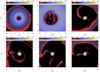 |
Fig. 1 Logarithm of the gas surface density in the base model, at time t = 3600 T. This model uses three overlapping polar grids, the outermost of which reaches out to 144 a. In the top panels the secondary star is located at the pericentre of its orbit. The bottom panels show the gas surface density at different orbital phases, with the secondary at apocentre in the central panel. The colour bar represents Σ in units of MA/a2. For the adopted system parameters, a density of 10−2 corresponds to ≈310 g cm−2. |
4 System dynamics
The gas surface density around the binary system is displayed in Figure 1, after 3600 binary periods, T. The top left panel includes the entire circumbinary disc, whose outer radius appears to be around 60 a. This radius, however, may vary according to the definitions. Integrating the gas surface density over the region r ≥ 9 a (i.e. beyond the tidal gap), 99.9% of the total mass is contained within r ≈ 52 a. Since the computational domain extends much farther, to r = 144 a, and the initial surface density is not truncated, this outer radius is not an artificial effect of limited computational domain or initial conditions; instead, it is determined by gas dynamics in the outer parts of the circumbinary disc. The estimated volume density of the gas at r ≳ 60 a is ≲10−20 g cm−3.
The top-centre panel of Figure 1 shows the gap region, whose outer edge has an azimuthally average radius r ≈ 9 a. The gap edge, however, is not circular and precesses about the centre of mass of the system. The region surrounding the two stars is shown in the top right panel, when the secondary star is at pericentre, and at other orbital phases in the bottom panels. The radius of the circumprimary disc is also ill defined; however, by integrating the gas surface density from the inner boundary of the grid (r = 0.04 a) out to r = 5 a, that is, inside the gap, 99.9% of the total mass is contained within r ≈ 0.22 a and 99.99% is contained within r ≈ 0.26 a.
The surface density of the gas in the system is undetermined, and our choices of initial conditions are obviously arbitrary. The application of a locally isothermal equation of state allows for hydrodynamical outcomes to be re-scaled, but the dynamics of the solids depends on the initial condition. Some upper bounds on the gas surface density can be estimated from the orbital evolution of the binary orbit driven by gravitational torques, under the assumption that the adopted orbit is close to final. We performed this experiment and allowed the orbit of the stars to change according to the torques exerted by the gas, and simulated the evolving orbits for approximately 80 binary periods. The results indicate that the orbital eccentricity varies at an average rate 〈de/dt〉 ≈ 10−7 yr−1, corresponding to an evolution timescale e/ė somewhat longer than the lifetime of the circumbinary disc. The semi-major axis of the binary evolves much more slowly. During the simulated period, the average rate is 〈da/dt〉 ≈ −3 × 10⁻⁸ a/yr, displaying 30% variations. The timescale a/ȧ is therefore much longer than the lifetime of the circumbinary gas. Over the duration of the simulations (≈3600 T), assuming these rates of change, the orbital eccentricity would have changed by several percent, whereas the semi-major axis would have changed by much less. Therefore, we can conclude that neglecting orbital variations in the models is a reasonable approximation.
4.1 Accretion rates of gas and fine dust
We estimated the accretion rates of gas towards the circumprimary disc using tracer particles (see Section 3.1), which provide a description of the evolution of the gas, starting from the region of their deployment. The transport can be quantified by using the conservation of the number of the tracers. Indicating with N their number density, conservation requires that
 (2)
(2)
where F = 𝒩u is the flux of tracers (u is the gas velocity). Equation (2), integrated over the disc region identified by the radial boundaries r1 and r2 (> r1), provides the accretion rate
 (3)
(3)
Since the geometry is two-dimensional, we note that the integral in Equation (2) is actually a surface integral, and hence the line integrals in Equation (3). Although d M/dt represents a number per unit time (the domain integral of 𝒩), it can be transformed into an accretion rate by converting the number density 𝒩 into a surface density (e.g. grams per square centimetre). This is accomplished by normalizing the initial number of tracers, using the mass of the region in which they are released. The interface fluxes, F1 and F2, are chosen as positive when directed towards the primary. In order to quantify the average values of mass transfer, all quantities in Equation (3) are time-averaged over ≈100 binary periods, T.
The two radii, r1 and r2, are chosen as representative of the outer boundary of the circumprimary disc (0.5 a) and of the gap (10 a), respectively. The actual radius of the circumprimary disc is shorter (see above) and the inner edge of the gap is not a circle. These details, however, are not important. The region between r1 and r2 is strongly perturbed by the tidal field of the stars, it has very low gas densities, and thus it is expected to not represent a significant source of gas for the circumprimary disc. If there is an influx of material towards the primary, it must come from beyond the gap edge. For this reason, precise values for r1 and r2 are unnecessary, as long as material flowing inside r1 supplies the circumprimary disc and material beyond r2 originates from the circumbinary disc. Equation (3) is used to derive the (time-averaged) integral of the inner flux, 〈F1〉, from the other two quantities, 〈dM/dt〉 and 〈F2〉, both of which are directly measured from the evolution of the tracers. As expected, tracer analysis indicates that |〈dM/dt〉| ≪ ʃ |〈r2F2〉|dϕ; we recall that d M/dt here is the variation of mass in the region between radii r1 and r2. Therefore, from Equation (3), we have
 (4)
(4)
Since the local-isothermal approximation allows for mass rescaling, indicating with Σref the average density between 10a and 20 a, in units of MA/a2, the average accretion rate of gas towards the circumprimary disc, estimated from the tracer analysis, is ≈7 × 10⁻² Σref (MA/T). For the values applied here, the accretion rate would be ≈2 × 10⁻⁸ M⊙ yr−1.
The ratio of the mass available beyond the gap edge to the accretion rate towards the circumprimary disc can be used to estimate the lifetime of the circumbinary disc. We note that this ratio is insensitive to the choice of the initial surface density, or Σref, because both terms scale as Σref, although it would depend on the applied gas viscosity and temperature (i.e. pressure scale height). This ratio, approximately 1.1 Myr, can be identified as an e-folding time for the evolution of the disc mass. Therefore, the estimate of the circumbinary disc lifetime would be around 3 Myr. This value, however, neglects other possible means of gas removal, such as energetic radiation from the stars (disc photo-evaporation).
The analysis of the tracers released inside 0.5 a indicates that there is no gas flowing out of the circumprimary disc, and hence no transfer of mass towards the secondary. This result also implies that the circumprimary disc can lose mass only via accretion towards the primary. A simple estimate of the inward transport in the circumprimary disc, based on steady-state accretion disc theory (Lynden-Bell & Pringle 1974; Pringle 1981), can be done by approximating the accretion rate to 3πΣν (averaged over the disc), which is on average roughly twice as large as the influx of gas from the circumbinary disc. A more accurate determination can be obtained by measuring the variation of the circumprimary disc mass during the same period of time over which tracers are evolved. This estimate, which is very well defined because of the sharp decline in the gas surface density beyond r ≈ 0.22 a, basically confirms that the disc is depleting (and the primary star is accreting) at a rate, ≈2.3 × 10⁻⁶ (MA/T), or ≈0.17 Σref (MA/T), about two times as large as the supply rate from the circumbinary disc. At this rate, neglecting again gas removal by stellar irradiation and assuming there was no supply of material from the circumbinary disc, the circumprimary disc would last only a few times 105 years, a length of time probably too short to allow the formation of giant planets. This outcome mostly depends on the small size of the disc and its limited mass reservoir. Therefore, the delivery of material from the circumbinary disc appears to be critical in this context. Because of external supply, the circumprimary gas would deplete until it attained a surface density such that the average product 3πΣν becomes comparable to the gas accretion rate provided by the circumbinary disc, which would ultimately dictate also the stellar accretion rate. In the set-up used for the base model, this equilibrium would entail a surface density around the primary a factor of ≈2 lower than that in Figure 1, and an actual lifetime of the circumprimary disc similar to that of the circumbinary disc, a few million years, which may be enough to form giant planets (e.g. Stevenson et al. 2022, and references therein).
As mentioned above, the secondary star is not fed gas by the circumprimary disc. It is, however, supplied by the gas inflow within the gap region. The fraction of this flux intercepted by the secondary is expected to be small and can be estimated directly from the simulations (see e.g. D’Angelo et al. 2006; D’Angelo & Marzari 2012). This accretion rate is almost three orders of magnitude lower than the accretion rate from the circumbinary disc towards the circumprimary disc. In terms of the reference density introduced above, the rate would be ≈10−4 Σref (MA/T). Figure 2 shows the average accretion rate of gas on the secondary, as a function of the true anomaly (see the figure caption for details). The accretion rate is modulated; the maximum delivery of gas occurs prior to apocentre passage (see e.g. Artymowicz & Lubow 1996).
As displayed in the top right and bottom panels of Figure 1, there is no permanent disc formation around the secondary, and the region has relatively low density. The average gas mass within 0.6 Hill radii of the secondary star is ≈2 × 10⁻⁴ Σref MA, which would correspond to ≈10−3 Earth’s masses for the values adopted in the model.
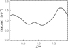 |
Fig. 2 Average accretion rate of gas on the secondary star as a function of the true anomaly, f, along its orbit. The results refer to the base model. In the plot the accretion rate is averaged over 100 orbital periods of the binary. The pericentre is at f = π. The units are Σref (MA/T), where Σref is the average density between 10 and 20 a, in units of MA/a2. |
4.2 Accretion rates of solids
The distribution of particles released in the circumbinary disc, superimposed to the surface density of the gas, is plotted in Figure 3. The particles are colour-coded by their radius, Rs, as explained in the figure caption. The smallest solids, Rs = 1 mm (red dots), remain confined beyond the gap edge and do not move inwards across the gap region (see left panel). Instead, the larger 1 and 10 cm particles can be transferred from the circumbinary to the circumprimary disc, as indicated by the green and orange dots in the right panel.
The segregation of the smallest particles outside the gap edge is a drag-driven effect, caused by the positive pressure gradient that develops at those radial locations. The local rotation rate of the gas exceeds, on average, that of the solids, generating a tail wind that tends to drive the particles outwards. Beyond the radial region of the positive pressure gradient, particles tend to drift inwards because gas rotation mainly generates a head wind on them. Therefore, the gap edge can represent a region of radial convergence for some particles, despite the complex dynamics of the gas. The converging effect is maximum for particles with a Stokes number of around unity, which are only partially coupled to the gas. At r ≈ 10 a, the thermodynamic conditions of the gas are such that 1 mm particles have Stokes numbers close to 1, and therefore are prone to be segregated outside the tidal gap edge. Since the Stokes number is inversely proportional to gas density, as the circumprimary disc depletes and densities reduce, 1 mm particles around the gap edge are expected to transition towards an uncoupled regime, and therefore at some point during the evolution they may be released and move towards the circumprimary disc.
The Stokes numbers of the 1 and 10 cm solids are ≫1, and hence they are less affected by drag at those locations. Their dynamics is mostly dictated by the gravity of the stars. They can acquire significant orbital eccentricity while orbiting in the circumbinary disc, which at some point allows them to cross the gap region and to be captured (via drag) by the high-density gas of the circumprimary disc.
Figure 4 shows the histograms of the semi-major axes of the particles in Figure 3, which allows a more quantitative assessment of the transfer of solids towards the primary star and the pile-up of 1 mm dust around the gap edge. We recall that the solid particles are initially deployed beyond 20 a from the primary. The histograms are stacked in order of increasing size: red for Rs = 1 mm particles, green for Rs ≤ 1 cm particles, and blue for all particles. In Figure 4 the number of 1 cm and 10 cm particles transferred to the circumprimary disc are similar. Nonetheless, the number of 10 cm particles in the circumbinary disc (i.e. beyond the gap edge) is smaller because they are more efficiently ejected from the system, indicating that their supply rate to the circumprimary disc is higher. During the last 50 orbits of the binary, the 10 cm solids are transferred towards the circumprimary disc at a rate about 1.8 times that of the 1 cm particles.
The particles that arrive in the circumprimary disc settle on low-eccentricity orbits after capture, as indicated by the histogram of orbital eccentricities in Figure 5. It is likely (because of the low density in the gap region) that particles are injected in the circumprimary disc on highly elliptical or even non-Keplerian orbits, and therefore arrive at velocities much higher than those of resident solids. These high relative velocities are likely to produce high-velocity collisions among particles, leading to fragmentation into smaller dust or coagulation into larger solids. We did not model collisions. However, the results in Figure 5 indicate that if particles avoid collisions, their orbital eccentricity is damped by gas drag over relatively short timescales. At the gas densities encountered in the circumprimary disc, 1–10 cm solids have Stokes number ≪1, and thus their dynamics quickly becomes closely coupled to that of the gas. The implication is that soon after arrival these particles become basically indistinguishable from an older resident population.
The solid particles are evolved for ≈200 T in the base model. The supply rate of 1 and 10 cm particles from beyond the gap region towards the primary initially grows over time, but it later becomes relatively steady. We measured the average (over the last ≈100 T of the solids’ evolution) supply rate of the 1 and 10 cm particles, from the variations in their number densities within the circumprimary disc. Once converted into accretion rates, they can be written as ≈80 σгef M⊕/T, for the 1 cm particles, and ≈380 σгef M⊕/T, for the 10 cm particles. In these estimates, the quantity σref represents the average surface density of solids, of the specific size, in the region between 10 a and 20 a, in cgs units. For comparison, the accretion rate of fine dust, estimated as a by-product of the accretion rate of gas derived in Section 4.1, can also be written as ≈σгef M⊕/T (after converting the units of the reference gas density Σгef).
For the circumbinary disc set-up applied in this paper, the often-quoted gas-to-solid mass ratio of 100 would yield σref ≈ 4 × 10⁻³ g cm−2. Strictly speaking, however, this density would apply to fine dust whose dynamics is closely coupled to gas dynamics, resulting in an accretion rate ~6 × 10⁻⁵ M⊕ yr−1. Since the dynamics of larger solids is uncoupled from that of the gas to a great extent, the estimate of σref should also account for the removal rate of solids from the region around the gap edge towards the farther regions of the disc and for the supply rate from those more distant regions. Therefore, a meaningful estimate of σref for 1 and 10 cm particles is more complex. If we simply assume a value of ~ 10−3 g cm−2, the accretion rates above become ~10−3 M⊕ yr−1 (Rs = 1 cm) and ~5 × 10⁻³ M⊕ yr−1 (Rs = 10 cm). We note, however, that all these estimates require that the entire reservoir of solids beyond the gap edge be available in the form of fine dust, 1 cm, or 10 cm particles. If instead the available mass was partitioned in the various size bins, as it is expected to be, the accretion rates in a given size bin would be lowered accordingly.
According to the estimated accretion rates and regardless of σref, the depletion time of ≈1 to ≈10 cm particles, from the circumbinary disc between 10 and 20 a, would be relatively short: from several hundred binary periods at the smaller end of the range to around one hundred binary periods at the larger end. If these timescales are too short compared to re-supply timescales of the solids from larger distances and from local coagulation and/or fragmentation, the flux of solids towards the primary may be also limited by these re-supply processes. The smaller ~1 mm grains that remain trapped beyond the gap edge may also contribute to re-supplying solids if they aid in the formation of larger particles.
Assuming a reference surface density σref ∼ 10−3 g cm−2, the equipartition of mass between the 1 and 10 cm particles, and an inefficient re-supply of solids to the 10–20 a disc region, about 30 M⊕ worth of solids would be transferred to the circumprimary disc from beyond the gap region. This mass should be added to that already available locally. If we estimate the local reservoir of solids in the circumprimary disc by re-scaling the average surface density of the gas (e.g. by a factor of 100), a few Earth masses of solids are available between 2 and 3 au from the primary star (with the parameters applied here).
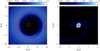 |
Fig. 3 Logarithm of the gas surface density in the base model with the particle positions superimposed: 1 mm (red), 1 cm (green), 10 cm (orange). All particles are initially located beyond 20 a. The panels show the gap region, its surroundings (left), and the circumprimary disc (right). The smallest particles do not cross the gap region to reach the circumprimary disc, whereas the larger particles do. The secondary star is at apocentre. The colour bar represents Σ in units of MA/a2. |
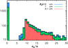 |
Fig. 4 Histogram of the semi-major axis of particles with different radii, as indicated in the legend. The histograms are stacked in order of increasing size: the red histogram includes particles Rs = 1 mm, the green histogram includes particles Rs ≤ 1 cm, and the blue histogram includes all particles. All solids start from beyond 20 a, and only the larger particles drift towards the circumprimary disc. The results shown refer to the base model. |
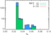 |
Fig. 5 Histogram of the orbital eccentricity of particles with different radii, as indicated. The histograms are stacked in order of increasing size, as in Figure 4. Only particles with a semi-major axis smaller than 0.5 a (i.e. orbiting inside the circumprimary disc) are represented. The smallest particles (1 mm) do not drift across the gap region as they are held back by the positive pressure gradient at the gap edge. The results refer to the base model. |
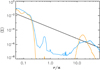 |
Fig. 6 Gas surface density averaged in azimuth around the primary, as a function of the radial distance, for the base model (α ≈ 0.001, orange curve) and a model with a higher viscosity parameter, α ≈ 0.005 (light blue curve). The black line represents the initial condition. The units of (Σ) are MA/a2. For the adopted system parameters, a density of 10−2 corresponds to ≈310 g cm−2. The secondary star is located at pericentre. |
4.3 High-viscosity model
Figure 6 shows a comparison between the average surface density of the gas around the primary star in the base model (orange curve) and another model with a higher turbulence parameter (see Section 3), α ≈ 0.005 (light blue curve). The two models are compared after an evolution of about 3300 binary periods. The mass and size of the circumprimary discs are similar in the two calculations. Because of the greater viscous stresses that oppose tidal forces exerted by the stars, the gap edge of the circumbinary disc extends inwards to about r ≈ 5 a, closer to the stars than in the base model. The densities in the circumbinary disc of the high-viscosity model are lower, but the disc extends farther out than it does in the base model. At large distances, the surface density also declines less abruptly than it does in the base model. Integrating Σ from r = 5 a outwards, over 95% of the total mass of the circumbinary disc is contained within r ≈ 100 a. However, the mass of the circumbinary disc is very similar in the two models.
The 2D density distribution around the stars is illustrated in Figure 7. The inner part of the circumbinary disc is shown in the left panel. Compared to Figure 1, the perturbations induced by the density waves propagating beyond the tidal gap are less prominent, as they are more efficiently damped by gas viscosity. As can be seen in the centre panel, the gap edge is highly asymmetrical around the binary, significantly more than in the base case (compare with the top centre panel in Figure 1). The smooth decline of Σ inside the gap (light blue curve in Figure 6) is mainly the result of the azimuthal average, around the primary, of the asymmetrical gas distribution within the gap region.
The secondary star is located at pericentre in Figures 6 and 7 (visible in the right panel), in correspondence of the buildup of gas in the gap at r = 0.6 a. Peak gas densities around the secondary are about 30 times as large as in the surrounding gap regions. Although not fully visible in Figure 6, similar density ratios are obtained around the secondary in the base model. Nonetheless, as indicated in the figure, the gas around the secondary is much denser than in the base model, by 2.5–3 orders of magnitude, an outcome mainly dictated by the much shallower gap of the high-viscosity model.
5 Implications for planet formation
In single-star systems, the dust density within the circumstellar gas is expected to decline with time, for all dust sizes, due to grain growth and dust transport processes (Testi et al. 2014). Grain growth is a progressive process whereby the smaller dust particles (initially micrometre-size) accumulate into larger pebble-size solids, which then can accumulate into planetesimals and possibly planets. Drag forces due to the interaction between grains and gas lead to a radial drift with a velocity relative to the gas that depends on the grain size and gas properties. The particles spiral towards the star on different timescales, although at some locations they may be halted by positive pressure gradients in the gas (e.g. due to gas density enhancements generated by the gravity of a planet). However, the rapid decay of the dust mass in circumstellar gas, expected on the basis of grain growth and radial drift, is not measured in the surveys of 1–3 Myr-old circumstellar discs observed by ALMA (Testi et al. 2014). It has been suggested (Bernabò et al. 2022; Turrini et al. 2019) that the growth of giant planets causes the formation of second-generation dust through collisions of leftover planetesimals, whose orbits are excited by the presence of planets. Under these circumstances, the dust density decline would start only 1–2 Myr after the formation of giant planets.
While in the case of single stars the dust density resurgence would just involve part of the primordial reservoir of solids (i.e. those formed out of the dust present in the circumstellar gas around the star since formation), in the binary star case with a circumprimary disc fed by an extended circumbinary disc, new ∼µm-size dust can be supplied during the lifetime of the circumbinary disc. Additionally, under the appropriate conditions, a non-continuous size distribution of particles, presenting a gap in some size range (millimeter sizes in our base model), would also be supplied to the circumprimary disc. These larger particles would presumably form out of coagulation–fragmentation exterior to the gas gap of the binary. The mass partition between ∼µm-size dust and 1–10 cm particles depend on the assumptions made and on the details of the coagulation–fragmentation processes. The segregation of particles beyond the gap edge is determined by the local pressure scale height, density, and viscosity of the gas. The range of particle sizes prevented from crossing the gap depends on the combinations of these parameters. As these properties of the gas evolve, segregated particles may be released from the gap edge region and move towards the circumprimary disc.
As mentioned at the end of Section 4.2, the circumbinary disc may contain a primordial reservoir of a few Earth masses worth of solids. If these solids turned relatively quickly and efficiently into planetesimals, which then assembled into a planet of a few Earth masses, the external supply of centimetre-size particles could aid in the formation of a larger (possibly giant) planet.
We estimated a total influx of solid mass, from the circumbinary disc, of around 30 M⊕ in the form of 1–10 cm particles. At an accretion efficiency of 10% (D’Angelo & Bodenheimer 2024), approximately 3 M⊕ would be added to a forming planet. Once it has attained several Earth masses, gas accretion may be significant, which could lead to growth beyond the pebble isolation mass of the planet (Morbidelli & Nesvorny 2012; Bitsch et al. 2018), halting any further inward drift of these particles. Therefore, even if the external supply of 1–10 cm particles was short-lived (see Section 4.2), significant amounts of pebble-size solids could accumulate in the outer part of the circumprimary disc. This situation could possibly lead to enhanced planetesimal formation (e.g. via streaming instability) (Johansen et al. 2015) or through turbulent gas concentration (Heng & Kenyon 2010; Hartlep & Cuzzi 2020). The latter mechanism may be particularly effective in the binary case since the companion’s perturbations excite strong spiral waves, which can contribute to turbulence generation in the gas. In the region beyond the planet’s orbit (out to the truncation radius if the system is compact, as is the one under study), a higher planetesimal formation rate may be expected, compared to the single-star case because of the steady supply of solids from the circumbinary disc. The resulting ring of planetesimals may trigger additional planet formation or, otherwise, lead to the production of a dense debris disc in the system in the proximity of the truncation radius of the circumprimary disc. This structure would be a significant observable feature, which may point to a past influx of solids from larger distances, and therefore to the past presence of a circumbinary disc. This feature could also point to the possible existence of planetary bodies inside the debris belt.
On a larger scale, if small grains remain trapped beyond the edge of the tidal gap until the circumbinary gas eventually disappears, they too may be observable as a debris disc. However, whether or not the original population of trapped particles is preserved depends on coagulation and fragmentation processes. The enhanced density of grains that are collected around those locations, as dust moves inwards from the farther regions of the circumbinary disc can ultimately produce a much broader size distribution of grains via collisions.
As mentioned above, solids arriving from the circumbinary to the circumprimary disc may have a non-continuous size distribution. This outcome is primarily determined by the local pressure gradient around the gap edge region and by the Stokes numbers of the solids. For example, the base model predicts a gap in the ~1 mm size range, because the Stokes numbers are around unity in that range. It is not clear how such a size distribution of grains would affect the turbulent accumulation of dust into planetesimals. It is possible that the resulting size distribution of planetesimals is different from that generated by a continuous distribution of dust grains, as is likely to occur in discs around single stars. It is difficult to argue whether or not these differences may actually discriminate between singlestar systems and compact binary systems. In general, the cores of giant planets can efficiently form from planetesimals from a few km to a hundred km in radius. As long as the reservoir of planetesimals include these bodies, formation would occur similarly in both types of systems. Such an outcome would likely be favoured by conditions in the circumbinary disc that allowed a more continuous size distribution of dust to move through the gap.
More extreme cases are, however, conceivable. If viscous stresses were much weaker than in the base model (e.g., smaller α), both gas and dust could be prevented from moving inwards. Not only would the availability of solids around the primary star be severely limited, but the gas would also dissipate quickly (in a few ×105 years, see Section 4.1). It is unlikely that giant planets would be able to form under these conditions.
An intermediate situation can be envisaged, in which the core of a giant planet would be able to form in the circumprimary disc, initiated by the local solids, and then aided by the supply of both gas and dust from the circumbinary disc. However, if the circumbinary disc were short-lived (e.g. ~1 Myr), the circumprimary disc would be short-lived as well, preventing the cores from fully developing into gas giants. As a result, gas-poor (or not-so-gas-rich) planets may form, such as Uranus and Neptune.
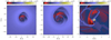 |
Fig. 7 Logarithm of the gas surface density in the high-viscosity model, at time t = 3300 T. As for the base model, the simulation uses overlapping polar grids that extend out to 144 a. The left and centre panels show the circumbinary disc, whereas the right panel shows the circumprimary disc. The secondary star is located at the pericentre of its orbit. The colour bar represents Σ in units of MA/a2. For the adopted system parameters, a density of 10−2 corresponds to ≈310 g cm−2. |
6 Conclusions
We simulated the evolution of the dust and gas in the environment surrounding a compact binary system, where a circumprimary disc co-exists with a large circumbinary disc. To model the evolution of the system, we used a high-resolution Eulerian code that employs a nested-grid technique to resolve different spatial scales, both much smaller and much larger than the stellar separation. In addition, tracers were used to better track the gas dynamics as it streams from the outer circumbinary disc to the inner circumprimary disc. A Lagrangian approach was used to simulate the evolution of the dust.
According to the model results, significant differences should arise when comparing the system evolution to that of a compact binary that is not supplied with gas and dust by a massive-enough circumbinary disc. There may also be differences with discs around single stars.
Assuming an average surface density of the circumbinary disc gas, between 10 a and 20 a, of  , in g cm−2, the accretion rate on the circumprimary disc is
  . This estimate is based on a model with a viscosity parameter α ≈ 0.001 and a flared disc whose H/r is 0.04 at a distance a from the primary star (see Section 3). The adopted set-up,
  , results in an accretion rate of
  . Without such a supply of gas, the lifetime of the circumprimary disc would be limited to a few times 105 years because of its low mass. The supply of gas from beyond the gap region extends this timescale to about 3 Myr, the lifetime of the circumbinary disc.
Dust grains would also be transferred from large distances to the circumprimary disc. Small (µm-size) grains would be carried by the accreting gas in which they are entrained, whereas larger, 1–10 cm grains would be driven across the gap mainly by the gravity of the stars. The applied conditions of temperature and viscosity cause ~1mm grains to be segregated beyond the gap edge because of the positive and large pressure gradient generated by the tidal field of the stars. This feature in the gas is conducive to segregation of solids with order-of-unity Stokes numbers due to gas–dust interactions.
As mentioned above, since the dynamics of the larger particles is mostly governed by gravity forces, they tend to acquire significant orbital eccentricity, which brings them towards the primary star. Solids delivered to the circumprimary disc on highly elliptical orbits may have spent a long enough time in the cold circumbinary gas to collect volatile materials (by condensation). Since their journey towards the circumprimary disc is rapid, they can carry, and deliver, significant amounts of volatile material to the circumprimary gas.
This continuing influx of gas and solids is likely to have relevant implications for the formation of giant planets. It is generally difficult to conceive that such planets may be able to form within a few 105 years (the lifetime of the isolated circumprimary disc). The extended lifetime (>1 Myr) would allow a core of several Earth masses to acquire a significant, or massive, envelope. The implication is that giant planets in compact binary systems are expected to be much more frequent in systems with a significant circumbinary disc. The base model would allow for about 30 M⊕ worth of solids to be transferred to the circumprimary disc, contributing to the accumulation of a giant planet core and to the formation of planetesimals.
The size distribution of the solids flowing across the gap is likely to depend on the density, temperature, and viscosity of the inner parts of the circumbinary disc. This distribution may be non-continuous, similar to that resulting from the base model. The ultimate effects on planetesimal formation of a non-continuous size distribution are difficult to predict. As long as planetesimals of a few to hundred km in radius are available, gas giant cores can be assembled. If a planet in the circumprimary disc exceeds its pebble-isolation mass, the continuing influx of solids may lead to the formation of additional planets or to the accumulation of a relatively massive debris or planetesimal belt in the proximity of the truncation radius of the circumprimary disc. This potentially observable feature would also represent a strong indication that the binary system was born with a circumbinary disc. Beyond the edge of the tidal gap, trapped grains may also form a debris belt, independent of the inner one, possibly providing further observational evidence of the past existence of a long-lived circumbinary disc.
Acknowledgements
The authors would like to thank an anonymous reviewer, whose constructive comments and suggestions helped improve the quality of this paper, and the Editor for helpful feedback. G.D. acknowledges support from NASA’s Research Opportunities in Space and Earth Science. Computational resources supporting this work were provided by the NASA High-End Computing (HEC) Program through the NASA Advanced Supercomputing (NAS) Division at Ames Research Center.
References
- Artymowicz, P., & Lubow, S. H. 1994, ApJ, 421, 651 [Google Scholar]
- Artymowicz, P., & Lubow, S. H. 1996, ApJ, 467, L77 [NASA ADS] [CrossRef] [Google Scholar]
- Bernabò, L. M., Turrini, D., Testi, L., Marzari, F., & Polychroni, D. 2022, ApJ, 927, L22 [CrossRef] [Google Scholar]
- Bitsch, B., Morbidelli, A., Johansen, A., et al. 2018, A&A, 612, A30 [NASA ADS] [CrossRef] [EDP Sciences] [Google Scholar]
- Chauvin, G., Beust, H., Lagrange, A.-M., & Eggenberger, A. 2011, A&A, 528, A8 [NASA ADS] [CrossRef] [EDP Sciences] [Google Scholar]
- D’Angelo, G., & Bodenheimer, P. 2013, ApJ, 778, 77 [Google Scholar]
- D’Angelo, G., & Bodenheimer, P. 2024, ApJ, 967, 124 [CrossRef] [Google Scholar]
- D’Angelo, G., & Marzari, F. 2012, ApJ, 757, 50 [CrossRef] [Google Scholar]
- D’Angelo, G., & Marzari, F. 2022, MNRAS, 509, 3181 [Google Scholar]
- D’Angelo, G., Lubow, S. H., & Bate, M. R. 2006, ApJ, 652, 1698 [CrossRef] [Google Scholar]
- Dutrey, A., Guilloteau, S., & Simon, M. 1994, A&A, 286, 149 [NASA ADS] [Google Scholar]
- Endl, M., Cochran, W. D., Hatzes, A. P., & Wittenmyer, R. A. 2011, AIP Conf. Proc., 1331, 88 [NASA ADS] [CrossRef] [Google Scholar]
- Hartlep, T., & Cuzzi, J. N. 2020, ApJ, 892, 120 [NASA ADS] [CrossRef] [Google Scholar]
- Heng, K., & Kenyon, S. J. 2010, MNRAS, 408, 1476 [NASA ADS] [CrossRef] [Google Scholar]
- Johansen, A., Mac Low, M.-M., Lacerda, P., & Bizzarro, M. 2015, Sci. Adv., 1, 1500109 [CrossRef] [Google Scholar]
- Jordan, L. M., Kley, W., Picogna, G., & Marzari, F. 2021, A&A, 654, A54 [NASA ADS] [CrossRef] [EDP Sciences] [Google Scholar]
- Kley, W., & Nelson, R. P. 2008, A&A, 486, 617 [NASA ADS] [CrossRef] [EDP Sciences] [Google Scholar]
- Lynden-Bell, D., & Pringle, J. E. 1974, MNRAS, 168, 603 [Google Scholar]
- Marzari, F., & Scholl, H. 2000, ApJ, 543, 328 [NASA ADS] [CrossRef] [Google Scholar]
- Marzari, F., & Thebault, P. 2019, Galaxies, 7, 84 [NASA ADS] [CrossRef] [Google Scholar]
- Marzari, F., Scholl, H., Thébault, P., & Baruteau, C. 2009, A&A, 508, 1493 [NASA ADS] [CrossRef] [EDP Sciences] [Google Scholar]
- Marzari, F., Baruteau, C., Scholl, H., & Thebault, P. 2012, A&A, 539, A98 [NASA ADS] [CrossRef] [EDP Sciences] [Google Scholar]
- Monin J. L., Clarke C. J., Prato, L., & McCabe, C. 2007, in Protostars and Planets V, eds. D. J. B. Reipurth, & K. Keil (Tucson, AZ: Univ. Arizona Press) [Google Scholar]
- Morbidelli, A., & Nesvorny, D. 2012, A&A, 546, A18 [NASA ADS] [CrossRef] [EDP Sciences] [Google Scholar]
- Mugrauer, M., Schlagenhauf, S., Buder, S., Ginski, C., & Fernández, M. 2022, Astron. Nachr., 343, e24014 [NASA ADS] [Google Scholar]
- Müller, T. W. A., & Kley, W. 2012, A&A, 539, A18 [Google Scholar]
- Nelson, A. F. 2000, ApJ, 537, L65 [Google Scholar]
- Nelson, A. F., & Marzari, F. 2016, ApJ, 827, 93 [Google Scholar]
- Neuhäuser, R., Mugrauer, M., Fukagawa, M., Torres, G., & Schmidt, T. 2007, A&A, 462, 777 [NASA ADS] [CrossRef] [EDP Sciences] [Google Scholar]
- Offner, S. S. R., Moe, M., Kratter, K. M., et al. 2023, in Protostars and Planets VII, eds. S. Inutsuka, Y. Aikawa, T. Muto, K. Tomida, & M. Tamura, Astronomical Society of the Pacific Conference Series, 534, 275 [NASA ADS] [Google Scholar]
- Paardekooper, S. J., Thébault, P., & Mellema, G. 2008, MNRAS, 386, 973 [NASA ADS] [CrossRef] [Google Scholar]
- Picogna, G., & Marzari, F. 2013, A&A, 556, A148 [NASA ADS] [CrossRef] [EDP Sciences] [Google Scholar]
- Pringle, J. E. 1981, ARA&A, 19, 137 [NASA ADS] [CrossRef] [Google Scholar]
- Schwarz, R., Funk, B., Zechner, R., & Bazsó, Á. 2016, MNRAS, 460, 3598 [Google Scholar]
- Shakura, N. I., & Sunyaev, R. A. 1973, A&A, 24, 337 [NASA ADS] [Google Scholar]
- Stevenson, D. J., Bodenheimer, P., Lissauer, J. J., & D’Angelo, G. 2022, PSJ, 3, 74 [NASA ADS] [Google Scholar]
- Su, X.-N., Xie, J.-W., Zhou, J.-L., & Thebault, P. 2021, AJ, 162, 272 [NASA ADS] [CrossRef] [Google Scholar]
- Testi, L., Birnstiel, T., Ricci, L., et al. 2014, in Protostars and Planets VI, eds. H. Beuther, R. S. Klessen, C. P. Dullemond, & T. Henning, 339 [Google Scholar]
- Thébault, P., Marzari, F., & Scholl, H. 2006, Icarus, 183, 193 [Google Scholar]
- Torres, G. 2007, ApJ, 654, 1095 [NASA ADS] [CrossRef] [Google Scholar]
- Trifonov, T., Lee, M. H., Reffert, S., & Quirrenbach, A. 2018, AJ, 155, 174 [Google Scholar]
- Turrini, D., Marzari, F., Polychroni, D., & Testi, L. 2019, ApJ, 877, 50 [NASA ADS] [CrossRef] [Google Scholar]
- van Leer, B. 1977, J. Computat. Phys., 23, 276 [NASA ADS] [CrossRef] [Google Scholar]
- Zeng, Y., Brandt, T. D., Li, G., et al. 2022, AJ, 164, 188 [NASA ADS] [CrossRef] [Google Scholar]
All Tables
Selected list of close binary systems hosting planets (from https://exoplanet.eu/planets_binary/).
All Figures
|
Fig. 1 Logarithm of the gas surface density in the base model, at time t = 3600 T. This model uses three overlapping polar grids, the outermost of which reaches out to 144 a. In the top panels the secondary star is located at the pericentre of its orbit. The bottom panels show the gas surface density at different orbital phases, with the secondary at apocentre in the central panel. The colour bar represents Σ in units of MA/a2. For the adopted system parameters, a density of 10−2 corresponds to ≈310 g cm−2. |
| In the text | |
|
Fig. 2 Average accretion rate of gas on the secondary star as a function of the true anomaly, f, along its orbit. The results refer to the base model. In the plot the accretion rate is averaged over 100 orbital periods of the binary. The pericentre is at f = π. The units are Σref (MA/T), where Σref is the average density between 10 and 20 a, in units of MA/a2. |
| In the text | |
|
Fig. 3 Logarithm of the gas surface density in the base model with the particle positions superimposed: 1 mm (red), 1 cm (green), 10 cm (orange). All particles are initially located beyond 20 a. The panels show the gap region, its surroundings (left), and the circumprimary disc (right). The smallest particles do not cross the gap region to reach the circumprimary disc, whereas the larger particles do. The secondary star is at apocentre. The colour bar represents Σ in units of MA/a2. |
| In the text | |
|
Fig. 4 Histogram of the semi-major axis of particles with different radii, as indicated in the legend. The histograms are stacked in order of increasing size: the red histogram includes particles Rs = 1 mm, the green histogram includes particles Rs ≤ 1 cm, and the blue histogram includes all particles. All solids start from beyond 20 a, and only the larger particles drift towards the circumprimary disc. The results shown refer to the base model. |
| In the text | |
|
Fig. 5 Histogram of the orbital eccentricity of particles with different radii, as indicated. The histograms are stacked in order of increasing size, as in Figure 4. Only particles with a semi-major axis smaller than 0.5 a (i.e. orbiting inside the circumprimary disc) are represented. The smallest particles (1 mm) do not drift across the gap region as they are held back by the positive pressure gradient at the gap edge. The results refer to the base model. |
| In the text | |
|
Fig. 6 Gas surface density averaged in azimuth around the primary, as a function of the radial distance, for the base model (α ≈ 0.001, orange curve) and a model with a higher viscosity parameter, α ≈ 0.005 (light blue curve). The black line represents the initial condition. The units of (Σ) are MA/a2. For the adopted system parameters, a density of 10−2 corresponds to ≈310 g cm−2. The secondary star is located at pericentre. |
| In the text | |
|
Fig. 7 Logarithm of the gas surface density in the high-viscosity model, at time t = 3300 T. As for the base model, the simulation uses overlapping polar grids that extend out to 144 a. The left and centre panels show the circumbinary disc, whereas the right panel shows the circumprimary disc. The secondary star is located at the pericentre of its orbit. The colour bar represents Σ in units of MA/a2. For the adopted system parameters, a density of 10−2 corresponds to ≈310 g cm−2. |
| In the text | |
Current usage metrics show cumulative count of Article Views (full-text article views including HTML views, PDF and ePub downloads, according to the available data) and Abstracts Views on Vision4Press platform.
Data correspond to usage on the plateform after 2015. The current usage metrics is available 48-96 hours after online publication and is updated daily on week days.
Initial download of the metrics may take a while.