| Issue |
A&A
Volume 695, March 2025
|
|
|---|---|---|
| Article Number | A109 | |
| Number of page(s) | 16 | |
| Section | Stellar structure and evolution | |
| DOI | https://doi.org/10.1051/0004-6361/202452820 | |
| Published online | 12 March 2025 | |
Modeling contact binaries
III. Properties of a population of close, massive binaries
1
Institute of Astronomy, KU Leuven, Celestijnenlaan 200D, 3001 Leuven, Belgium
2
Department of Astrophysics and Planetary Science, Villanova University, 800 E Lancaster Ave., Villanova, PA 19085, USA
3
Argelander-Institut für Astronomie, Universität Bonn, Auf dem Hügel 71, D-53121 Bonn, Germany
4
Max-Planck-Institut für Radioastronomie, Auf dem Hügel 69, D-53121 Bonn, Germany
5
Leuven Gravity Institute, KU Leuven, Celestijnenlaan 200D Box 2415, 3001 Leuven, Belgium
⋆ Corresponding author; This email address is being protected from spambots. You need JavaScript enabled to view it.
Received:
30
October
2024
Accepted:
3
January
2025
Abstract
Context. Among massive stars, binary interaction is the rule rather than the exception. The closest binaries – those with periods of less than ∼10 days – undergo mass transfer during core-hydrogen burning, with many of them experiencing a nuclear-timescale contact phase. Current binary population synthesis models predict the mass-ratio distribution of contact binaries to be heavily skewed toward a mass ratio of unity, which is inconsistent with observations. It has been shown that effects of tidal deformation due to the Roche potential and energy transfer in the common layers of a contact binary alter the internal structure of close binary components. However, previous population studies neglected these effects.
Aims. We aim to model a population of massive binary stars that undergo mass transfer during core-hydrogen burning, while consistently considering the effects of tidal deformation and energy transfer in contact phases.
Methods. We used the MESA binary-evolution code to compute large grids of models with primary star masses of 8 − 70 M⊙ at solar metallicity. We then performed a population-synthesis study to predict distribution functions of the observational properties of close binary systems, focusing in particular on the mass and luminosity ratio distribution.
Results. We find that the effects of tidal deformation and energy transfer have a limited effect on the predicted mass-ratio distribution of massive contact binaries. Only a small fraction of the population have their mass ratio significantly shifted toward a more unequal configuration. However, we suggest that orbital hardening could affect the evolution of contact binaries and their progenitors, and we advocate for a homogeneous set of observed contact binary parameters.
Key words: binaries: close / stars: evolution / stars: massive
© The Authors 2025
 Open Access article, published by EDP Sciences, under the terms of the Creative Commons Attribution License (https://creativecommons.org/licenses/by/4.0), which permits unrestricted use, distribution, and reproduction in any medium, provided the original work is properly cited.
This article is published in open access under the Subscribe to Open model. This email address is being protected from spambots. You need JavaScript enabled to view it. to support open access publication.
1. Introduction
Among massive-star (Minit ≳ 8 M⊙) populations, the binary fraction is observed to be very high, and the majority of stars are born in systems that will undergo strong interactions (Mason et al. 2009; Sana et al. 2012, 2013, 2014; Kobulnicky et al. 2014; Dunstall et al. 2015; Guo et al. 2022; Lanthermann et al. 2023). The observed period distribution of these binaries is consistent with it being (logarithmically) flat, 𝒩(log p)∼(log p)0, over periods ranging from one to several hundred days, meaning a significant fraction of binaries have short initial periods (pinit ≲ 10 d, Sana et al. 2013; Almeida et al. 2017; Villaseñor et al. 2021; Banyard et al. 2022). Many population synthesis studies show that such binaries interact on the main sequence, following so-called Case-A evolution (e.g., Pols 1994; Vanbeveren et al. 1998; Nelson & Eggleton 2001; de Mink et al. 2013; Sen et al. 2022).
Accurately modeling binary interaction is of paramount importance in order to understand the evolution of massive stars (Marchant & Bodensteiner 2024). Close binary interaction leads to phenomena that cannot be explained by single-star models such as stellar mergers and their associated magnetism (Schneider et al. 2019; Frost et al. 2024), super-luminous supernovae (Yoon & Langer 2005; Yoon et al. 2006; Aguilera-Dena et al. 2018, 2020), and results in directly observable interaction products such as stripped stars (e.g., Shenar et al. 2020; Bodensteiner et al. 2022; Drout et al. 2023 and short-period Wolf-Rayet binaries (Hainich et al. 2014; Pauli et al. 2022). Furthermore, close massive-binary evolution can yield gravitational-wave merger events through various channels. In particular, the chemically homogeneous evolution channel (Marchant et al. 2016; Mandel & de Mink 2016) favors very close binaries – that is, those with periods of around 1 d – which in most cases means such binaries experience extended periods of contact evolution.
In very close binary systems (p ≲ 2 d), a contact phase is likely to occur (Wellstein et al. 2001; Menon et al. 2021; Henneco et al. 2024a). Such phases are characterized by both stars overflowing their respective Roche lobes (RLs) simultaneously. In this configuration, the outer layers of the stars are heavily deformed by the tidal interaction between the companions. Additionally, there is thermal contact in the common layers of a contact binary, which allows for the transfer of energy between the components just as the mechanical contact allows for mass transfer (MT).
Hundreds to thousands of low-mass contact binaries, called W Ursae Majoris (W UMa) stars, have been discovered thanks to both targeted and all-sky photometric surveys (Eggen 1967; Binnendijk 1970; Szymanski et al. 2001; Selam 2004; Paczynski et al. 2006; Graczyk et al. 2011, 2018). Conversely, only a few dozen contact systems with massive components are known, resulting from the MACHO survey (Alcock et al. 1997), the Tarantula Massive Binary Monitoring (TMBM, Almeida et al. 2015, 2017; Mahy et al. 2020a,b), and the analysis of several galactic objects (e.g., Polushina 2004; Penny et al. 2008; Lorenzo et al. 2014, 2017; Yang et al. 2019; Abdul-Masih et al. 2021; Mahy et al. 2020a; Li et al. 2022a). Contact-binary light curves are characterized by smooth, near-sinusoidal variability, without flattened (partial) eclipses, signaling that the components are of comparable size and temperature. Using a Wilson-Devinney-like method (Wilson & Devinney 1971, and later updates), the analysis of the light curve allows, among other things, the determination of the overflow degree, (R − RRL)/RRL, of the components. Unfortunately, this value is rather uncertain from the light curve alone, and it is sometimes unclear whether a system is in true contact or only in near contact (e.g., Hilditch et al. 2005; Mahy et al. 2020a). A spectroscopic characterization can be performed to obtain dynamical masses and thus an independent constraint on the mass ratio and the projected physical separation. The combination of these analyses, especially when accounting for the tidally distorted nature of the photosphere, provides the best measurements of contact-binary parameters (Abdul-Masih et al. 2020, 2021).
In the literature, most efforts to theoretically model contact binaries are focused on the W UMa stars. Many models include a prescription of energy transfer (e.g., Lucy 1968; Biermann & Thomas 1972; Flannery 1976; Shu et al. 1976; Kähler 1989), but some turned out to either produce inaccurate light curves or contain inconsistencies. Unfortunately, models that are applicable to massive stars with radiative envelopes are more limited. Shu et al. (1976) provided the contact-discontinuity model, but it is challenged by Papaloizou & Pringle (1979), Hazlehurst & Refsdal (1980), and Hazlehurst (1993). Given the problems in developing a complete theory of contact-binary structure, many recent studies that focused on close massive binary evolution and included contact phases, such as de Mink et al. (2013), Marchant et al. (2016), Menon et al. (2021), Sen et al. (2022), and Henneco et al. (2024a), ignored energy transfer in the common layers of a contact system. The models find that contact phases can occur in both thermally unstable and thermally stable evolution. In the former, a rapid MT phase causes the accretor to swell beyond its RL as it falls out of thermal equilibrium, while in the latter the evolution is dominated by the nuclear timescale of the system. However, these state-of-the-art models have trouble reproducing the observed mass-ratio distribution of contact systems. While they indicate that once nuclear-timescale contact is engaged the binary should equalize rapidly (Menon et al. 2021), long-term monitoring of the period derivative shows that the orbit evolves on a nuclear timescale (Abdul-Masih et al. 2022; Vrancken et al. 2024). However, Fabry et al. (2023) showed that for particular systems, energy transfer in radiative envelopes can alter the mass-ratio evolution of massive contact systems and has the possibility to relieve part of the discrepancy between models and observations.
In this work, we used the methodology developed in Fabry et al. (2022, 2023), which we henceforth refer to as Paper I and Paper II, respectively, to consistently take into account tidal deformation of close binary components and energy transfer in contact phases. We computed a grid of short-period, massive binary-evolution models and investigate the effect of energy transfer on the mass-ratio distribution of contact systems. The paper is organized as follows. Section 2 describes the setup of the stellar-evolution calculations, the assumptions concerning stellar and binary physics, and the initial and termination conditions; and we specify the explored parameter space to provide population predictions. Section 3 presents and discusses the results obtained from the population-synthesis modeling, while Sect. 4 gives concluding remarks.
2. Methods
We used the detailed binary-evolution code MESA, version 22.11.1 (Paxton et al. 2011, 2013, 2015, 2018, 2019; Jermyn et al. 2023), to compute grids of models that undergo Case-A MT; from this, we assembled a synthetic population. All models were computed at solar metallicity, Z⊙ = 0.0142, with metal fractions following those of Asplund et al. (2009). The parameters to be varied in each grid are the initial primary mass, M1,init, initial mass ratio, qinit = M2,init/M1,init, and the initial period, pinit. For initial primary mass, we sampled M1,init = {8, 9, 10, …, 19} ∪ {20, 22, 24, …, 48} ∪{50, 52.5, 55, …, 70} M⊙, which is chosen to cover the mass range of all observed (near) contact binaries (accounting for significant mass loss of the most massive stars). The initial mass ratio is qinit = 0.6 − 0.975, spaced uniformly with Δqinit = 0.025, while the initial period is pinit = 0.5 − 8 d, spaced logarithmically with Δlog(p/d) = 0.04. We computed three grids with the following parameter variations: one that includes the effect of energy transfer (ET) and tidal deformation, one without ET but with tidal deformation, and one without ET and using the single-rotating star deformation corrections from Paxton et al. (2019). This amounts to a total of 53568 detailed binary-evolution models. We required these extensive grids to precisely identify where ET has the greatest impact in the parameter space. Throughout the discussion, we refer to the models that include ET and tidal deformation as the “ET models”, those that do not include ET (but still use the tidal deformation) as the “no-ET models”, and those that use the single-rotating-star deformation as the “single-rotating models”.
2.1. Physical assumptions in MESA
We used a similar setup of the MESA code to that of Paper II; that is, we used the same microphysics, convection and overshoot model, wind prescription, deformation geometry, and mass- and energy-transfer calculations. We briefly present the general setup, while the significant changes with respect to Paper I and Paper II are listed at the end of this section.
In terms of microphysics, we used the OPAL radiative opacities from Iglesias & Rogers (1993, 1996), and Ferguson et al. (2005) for low-temperature opacities. For high temperatures, we used the Compton scattering opacities from Poutanen (2017) and electron conduction opacities from Cassisi et al. (2007) and Blouin et al. (2020). The equation of state is a blend of elements from Saumon et al. (1995), Timmes & Swesty (2000), Rogers & Nayfonov (2002), Potekhin & Chabrier (2010), and Jermyn et al. (2021), specified in Jermyn et al. (2023) (except that we exclude the FreeEOS table). We used the basic nuclear-reaction network involving the species 1H, 3He, 4He, 12C, 14N, 16O, 20Ne, and 24Mg, with reaction rates taken from the JINA (Cyburt et al. 2010) and NACRE (Angulo et al. 1999) libraries, with weak interaction tables from Fuller et al. (1985), Oda et al. (1994), and Langanke & Martínez-Pinedo (2000). Electron screening is computed as per Chugunov et al. (2007), and thermal-neutrino losses are taken from Itoh et al. (1996).
Wind-mass loss is computed as per Brott et al. (2011). If the surface-hydrogen fraction is X > 0.7, the mass-loss rate depends on the surface temperature. If the temperature is above the iron bi-stability jump (as calibrated by Vink et al. 2001), the mass-loss rate is that of Vink et al. (2001), while below that temperature, the maximum of the rates of Vink et al. (2001) and Nieuwenhuijzen & de Jager (1995) is chosen. For surface-hydrogen fractions of X < 0.4, the mass-loss prescription from Hamann et al. (1995) is used and reduced by a factor of ten. Between 0.4 < X < 0.7, the mass-loss rate is linearly interpolated between the above schemes. Wind MT is accounted for through the Bondi-Hoyle mechanism (Bondi & Hoyle 1944), as implemented by Hurley et al. (2002).
Convective regions are determined following the Ledoux criterion (Ledoux 1947), where the mixing length theory of Vitense (1953) and Böhm-Vitense (1958) is applied (as described by Cox & Giuli 1968). Step overshooting is used as calibrated by Brott et al. (2011), where the diffusion coefficient from 0.01 pressure scale heights inside the boundary is kept constant at 0.335 pressure scale heights outside the convective-core boundary. We account for the semiconvective instability as treated by Langer et al. (1983) and thermohaline mixing from Kippenhahn et al. (1980), both of which have an efficiency of unity: αsc = αth = 1.
MT in semi-detached configurations is computed implicitly by requiring the donor to stay just below its RL radius (as approximated by Eggleton 1983). For contact configurations, the MT rate is adjusted so that the radii of the stars share an equipotential surface, amounting to a relation of
 (1)
(1)
where r = (R − RRL)/RRL is the relative RL overflow of a component. Within the grids with the tidal deformation corrections, we used the integrations of Paper I to construct F, while in the case of the single-rotating star corrections we used F(q, x) = q−0.52x, as in Marchant et al. (2016). ET was computed as in Paper II, assuming there is an efficient energy flow from one component to the other in the layers near the RL equipotential. Energy is redistributed so that each component radiates a fraction of the total luminosity L1 + L2 proportional to its surface area S and surface-averaged effective gravity ⟨g⟩; this is because we assumed von Zeipel’s theorem of radiative equilibrium holds (von Zeipel 1924). The combination of using the tidal-deformation corrections and efficient ET ensures shellularity of the shared envelope of a contact-binary model Paper II.
With respect to Paper I and Paper II, we made the following modifications to the modeling setup.
-
We do not assume rigid-body rotation throughout the evolution, so differential rotation was allowed. However, since we expected fast tidal synchronization for very close binaries (Zahn 1977), we uniformly modified the angular momentum of the star on the timescale of the orbital period, p:
 (2)
(2)Here, Δt is the timestep of the evolution; j and irot are the current angular momentum and the moment of inertia of the stellar layer, respectively; and ωorb = 2π/p is the orbital angular velocity. We modeled spin-orbit coupling to conserve total angular momentum, so the required angular momentum to synchronize both stars in this manner was then subtracted from the orbital angular momentum. Given that Δt is much longer than the orbital period in evolutionary calculations (years to thousands of years versus days), Eq. (2) specifies efficient tidal synchronization. We thus expect little departure from solid-body rotation in our very close binary simulations, since processes that cause departures from it operate on longer timescales than the orbital one.
-
We also allowed for rotational mixing in our models. We included Eddington-Sweet circulation (Eddington 1925; Sweet 1950), the Goldreich-Schubert-Fricke instability (Goldreich & Schubert 1967; Fricke 1968), and both the dynamical- and secular-shear instability (Zahn 1992; Endal & Sofia 1978), all following the implementation of Heger et al. (2000).
-
We reduced the parameters of mixing-length theory to αMLT = 1.5 and the semiconvective efficiency to αsc = 1; this allowed us to be in line with Menon et al. (2021).
-
When using the single-rotating-star deformation corrections, we set up the code to follow the settings used in Menon et al. (2021) as closely as possible. No ET is applied for this grid of models. The specific moment of inertia of a stellar shell of radius rΨ is evaluated simply as irot = 2/3 rΨ2, while the structure corrections fP and fT follow the analytical fits of Paxton et al. (2019), with the modification that the corrections are bound to their values at 60% critical rotational velocity. We emphasize that this does not mean that a model cannot rotate faster than this limit, only that the structure corrections are limited to values above 0.74 and 0.93 for fP and fT, respectively. From the results of Paper I, the single-rotating-star corrections slightly underestimate the deformation as compared to the tidal corrections.
2.2. Binary initialization
Once initial masses and a period are selected, the binary model is initialized as follows. Non-rotating, single-star models of mass M1,init and M2,init = qM1,init are interpolated from pre-computed zero-age-main-sequence (ZAMS) models of solar metallicity and a helium content of Y = 0.2703. We set the eccentricity to zero as we expected circular orbits for close binaries (Zahn 1975). The single-star models are then spun up to the appropriate Keplerian angular velocity ωorb. Since the models are brought out of thermal equilibrium due to the spin up, what follows is a thermal relaxation period onto the true ZAMS of the models, during which MT, ET, and any other mass loss is turned off. We also kept the period constant to the initial value and enforce rigid-body rotation at the orbital angular velocity. We define the ZAMS as the point where the luminosity of both stars is within 1% of their nuclear luminosity. When this condition is reached, we make a decision depending on the overflow rate of the stars.
First, if both stars are within their respective RLs, the simulation proceeds as normal and without further intervention. Second, if at least one star overflows its RL, this means that MT must have started in the pre-main-sequence (PMS) phase. We do not take these models into account in the main body of the paper, but we discuss them in Appendix A. Finally, if one of the stars overflows the second Lagrangian point (L2OF) at the ZAMS, we terminated the simulation immediately as we assume a merger would have happened on the PMS.
2.3. Outcomes and termination
The outcome of our simulations broadly falls into the following three categories.
-
The binary reaches L2 in a contact configuration. In this situation, we assume mass loss will start from L2, carrying away a large amount of specific angular momentum (Kuiper 1941), which we expect results in a merger on a short timescale. We stop the simulation at this point and classify these systems as “mergers”. A variant of this outcome is when the MT calculation determines that Ṁ is a very high value. We chose to take a limiting value of Ṁ = 10−1 M⊙ yr−1 across the whole grid. MT rates higher than this value are at least two orders of magnitude above the thermal timescale MT rates of massive main-sequence stars (except perhaps for the highest masses in our grid, where Ṁthermal ≈ 5 × 10⁻³ M⊙ yr−1), and we expect MT to evolve toward dynamical-timescale MT, which is associated with highly nonconservative evolution, likely leading to a merger.
-
One of the stars (most likely the initially more massive one) reaches core-hydrogen exhaustion without triggering a merger. At this point, the star will start undergoing rapid evolution, and we stop the simulation, calling these “(main-sequence) survivors”.
-
The simulation can encounter numerical difficulties, for example by failing to reach convergent models during the evolution. In this case, we halt the simulation and signal this system encountered an “error”.
2.4. Population synthesis computations
The probability density, 𝒫, of finding systems in a certain configuration ϑ0 is then proportional to the weighted contributions in that configuration,
 (3)
(3)
where each of the models, 𝒩, are considered only at the configuration ϑ = ϑ0, using the Dirac delta function, δ. If the required configuration is characterized by a single quantity parameterized by time, ϑ = ϑ(t), we can simplify Eq. (3) by transforming the delta function under composition with a function g:
 (4)
(4)
where we sum over the (simple) roots of g. Therefore,
 (5)
(5)
 (6)
(6)
This shows that the probability density is inversely proportional to the velocity at which the quantity in question changes at the time where ϑ = ϑ0, and we sum the contributions from all times ti at which ϑ = ϑ0. For n-dimensional configurations, ϑ, the mathematics is not as straightforward to write down, but the result is that we should sum over the (n − 1)-dimensional hypersurface where ϑ = ϑ0, which may consist of multiple disconnected parts (just as there might be different roots in the 1D case).
The probability density is weighted with factors 𝒲𝒩 coming from the likelihood of this model being created from the star- and binary-formation processes. Since we vary the initial primary mass, initial mass ratio, and initial period, and take into account the star-formation-rate (SFR) history, the total (relative) weight is given by
 (7)
(7)
The individual weights are taken from models of observed young populations. Specifically, we adopted
 (8a)
(8a)
 (8b)
(8b)
 (8c)
(8c)
 (8d)
(8d)
coming from the Salpeter initial-mass function (Salpeter 1955; Kroupa 2001; Bastian et al. 2010) and the modeled mass-ratio distributions found from a sample of O-type stars (Sana et al. 2012; Shenar et al. 2022). No sample of observed binaries covers periods shorter than 1 d, so we adopted Öpik’s law (Öpik 1924), 𝒲pinit = 1/pinit, which is close to the findings of Almeida et al. (2017). Unless the index of the period-distribution power law is positive and high, which is not supported by any observational sample of young, massive stars, short-period binaries are favored over longer ones. We used no twin binary excess in our setup, since high-mass stars have small twin fractions (Sana et al. 2012; Moe & Di Stefano 2017). The age prior indicates whether we assumed a constant SFR.
Given we have a grid of a discrete number of models, each grid point represents a finite area of the birth distributions in Eq. (8). In particular, we compute
 (9)
(9)
for the contribution of the model of initial primary mass M1,init , and the upper and lower bounds are taken from between our grid points. For points on the edge of the grid, we linearly extrapolated the spacing outward and then used Eq. (9) as usual. In this way, the model with an initial primary mass of 8 M⊙ has Mupper = 8.5 M⊙ and Mlower = 7.5 M⊙, while the model of highest initial mass has Mupper = 71.125 M⊙ and Mlower = 68.875 M⊙. Since our grid is logarithmically spaced in an initial period and uniformly spaced in the initial mass ratio, given the assumed weights, each model has the same contribution in those dimensions.
With this setup, we can compute the probability of finding a contact binary within a bin of a certain observed period and mass ratio:
 (10)
(10)
where we define
 (11)
(11)
as the observed mass ratio. Additionally, we only filtered the models to times where they are in a contact configuration: R1 ≥ RRL, 1 and R2 ≥ RRL, 2.
3. Results and discussion
After computing the binary-evolution models according to the methods described in Sect. 2, we obtained the following outcomes. Figure 1 shows the termination conditions of the ET models of initial masses of 26 M⊙ and 62.5 M⊙ (the results for the full grids are available on the Zenodo repository). We observe a good completion rate, with less than 9% of models with ET failing and 5% of models without ET failing. Furthermore, the lower mass models in the pinit = 1.7 − 2.1 d range that fail do so very close to the TAMS. Hence, we do not expect them to contribute significantly to the time spent in contact.
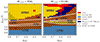 |
Fig. 1. Termination conditions of 26 M⊙ and 62.5 M⊙ models that use ET as function of the initial mass ratio qinit = M2,init/M1,init and initial period pinit. In color we indicate the models that experience L2OF at the ZAMS (light blue), those that experience L2OF during the main sequence (orange, “mergers”) or experience a MT rate above 10−1 M⊙ yr−1 (dark blue), those that survive the main sequence without experiencing L2OF (yellow), and those terminate with a numerical error (red). Forward-hatched models experience contact during their main-sequence evolution, while backward-hatched models overflow their RL at the ZAMS. Outlined in white are five classes (“Class 0-IV”) of systems determined by their qualitative evolution (see Sect. 3.1). |
We also note that a large fraction of models experience L2OF or RLOF at the ZAMS. We expect all of these models to interact on the PMS. Furthermore, we expect the L2OF systems to merge even before hydrogen starts burning. Those systems would then not be observable as binaries with components on the main sequence, and we classify these as Class 0 in Fig. 1. Because the models that experience RLOF at the ZAMS were given an ad hoc treatment to smoothly let MT start as the stars approach to their initial period, we do not include them in the population synthesis of the main text. We classify them under Class 0 too, and we briefly discuss them in Appendix A.
3.1. Example models
Apart from the models that interact on the PMS, which we call Class 0 models, we identify four other categories of evolution for our Case A binaries, indicated as Classes I–IV in Fig. 1, which we discuss below.
The Class I models contain those that interact early on the main sequence, which were dubbed System 1 by Menon et al. (2021). Here, the more massive star starts fast Case-A MT before an appreciable fraction of the main sequence is traversed. Contact is engaged immediately, and as soon as both stars regain thermal equilibrium after the rapid MT event, MT reverses and the system promptly evolves to mass ratios close to unity. We show an example of this type of evolution in Fig. 2, which has initial conditions of  , pinit = 1.15 d, and qinit = 0.7. We note that ET has little impact on the long-term evolution of this system. The small age difference seen in the purple, single-rotating curve is due to those stars being slightly more compact at the same mass and evolutionary stage Paper II; hence, interaction occurs slightly later.
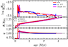 |
Fig. 2. Evolution of a Class I system with initial parameters |

The Class II systems are those of low-to-moderate mass that start MT after an appreciable fraction of the main sequence has been traversed. Such systems were dubbed System 2 by Menon et al. (2021), and we give an example evolution (M1, init = 30 M⊙, qinit = 0.9, pinit = 1.52 d) in Fig. 3. Here, a fast Case-A MT phase is followed by a slow Case-A MT phase from the primary, which drives the mass ratio further off unity. This is the classical Algol phase, which was recently studied in detail by Sen et al. (2022) (see also Pols 1994; Vanbeveren et al. 1998; Wellstein et al. 2001). Then, as nuclear-timescale contact is engaged once the accretor fills its RL, MT reverses, which eventually equalizes the masses of the components. This kind of evolution was shown in detail in Paper II. ET has a significant effect for such systems, because it moderates the MT rate at the point where nuclear-timescale contact is engaged. In particular, in both the example given here and in Paper II, ET delays the mass equalization, so models with ET are more likely to be observed at unequal mass ratios. Similarly to the Class I example in Fig. 2, the model with the single-rotating-star corrections interacts slightly later, but otherwise equalizes its mass ratio as quickly as the no-ET model.
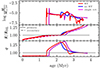 |
Fig. 3. Evolution of a Class II system with initial parameters |
There exists some uncertainty in the literature on the width and location of the energy transferring layers in both low-mass and massive contact binaries (e.g. Zhou & Leung 1990; Li et al. 2004; Paper II). In Appendix B, we show that because the evolution of the Class II model is on the nuclear timescale, its properties are insensitive under different assumptions on the width of the ET layer. Therefore, we expect the properties of our contact-binary population, which is dominated by nuclear-timescale contact phases, to be only weakly dependent on the precise implementation of ET.
The Class II model also shows the stark difference between the evolution of massive contact binaries evolve and low-mass W UMa binaries. The main reasons are the differing thermal structures of the envelope and differing timescales of evolution. For long-lived massive contact systems, the nuclear timescale dominates the evolution. The MT rate is rather low, so the radiative envelope can easily adjust to slight changes in the ET rate. The core of the accretor rejuvenates efficiently due to strong overshooting, which adjusts the nuclear luminosity, and the system therefore evolves to the equilibrium state of equal masses. In low-mass contact binaries, however, as modeled following Flannery (1976) and Lucy (1976), even though the secular evolution of the system as a whole is on the nuclear timescale, the separate components evolve on the thermal timescale. During a contact phase, the convective envelope of the lower mass component in the system gains energy and expands greatly. This causes the lower mass star to become the mass donor in the system, rather than the more massive star; thus, the mass ratio becomes more extreme, instead of more equal as to does in the massive binary case. Li et al. (2004, 2005), and Yakut & Eggleton (2005) computed models of low-mass contact binaries that show thermal relaxation oscillations. In Appendix C, we show a low-mass evolution model with a prescription of angular momentum loss by magnetic braking, but otherwise a similar setup to Sect. 2; it shows that our model also exhibits thermal oscillations and evolves to more unequal masses.
The Class III systems are those that spend less than 5% of their total lifetime in contact phases. They occur at all masses when the Case A MT starts late on the main sequence, corresponding to initial orbital periods of pinit ≳ 2 − 3 d. Most models in this regime even avoid contact during the fast Case A (the exceptions being at low mass and low-mass ratio: M1,init ≲ 40 M⊙, qinit ≲ 0.7). All models go through a fast Case A MT and a subsequent Algol phase. Then, at a high initial period, and/or low initial mass ratio, the primary of the system reaches core-hydrogen exhaustion. Another scenario in this class is that contact is engaged as the accretor in the Algol reaches its RL; but, conversely to Class II, the contact phase is limited because the components increase in size significantly as they reach the end of the main sequence. The models in this category are thus most likely observable as pre-interaction or Algol systems.
Finally, the Class IV systems we distinguish are the (very) massive models (M1,init ≳ 45 M⊙) that interact early on the main sequence. The models in this regime suffer significant mass and angular-momentum loss due to strong stellar winds (recall that we modeled galactic binaries), and they also rotate quickly because of their very short periods and quick synchronization. Both these properties have the effect of keeping the radius-to-RL size small, because these models evolve nearly chemically homogeneously, and the wind mass loss causes orbital widening. An example of this evolution is shown in Fig. 4. Models in this class engage in nuclear-timescale contact, but eventually the orbit widens enough for the stars to detach, and they avoid a main-sequence merger. These models are binary black-hole merger progenitors (Marchant et al. 2016). For the specific model shown in Fig. 4, the secondary reaches core-hydrogen exhaustion first.
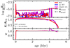 |
Fig. 4. Evolution of a Class IV system with initial parameters |
3.2. Population properties
From our model outputs, we compute the probability of finding contact systems with a certain observed period and mass ratio. This amounts to evaluating Eq. (10) for our grids. Figure 5 shows the result. First, we note that the models in all grids heavily cluster toward the parameters (qobs, pobs) = (1, 1 d), similarly to the findings of Menon et al. (2021). Overall, the three grids of models have a similar probability density distribution. To better highlight the differences between the distributions, we draw highest density intervals (HDIs) on the panels of Fig. 5 (shown by black lines) to indicate in which regions a certain fraction of models would be found. Only in the 90th percentile do we see a noticeable shift. Taking the single rotating models as baseline, we see that including the tidal deformation corrections (but no ET) slightly moves the lowest observed mass ratio in toward one; while using tidal reformation and ET moves it toward lower mass ratios. However, when computing the expected mass ratio,  , from our PDFs, we obtain
  for the single-rotating models,
  for the no-ET models, and
  for the ET models. The effects of tidal deformation and energy transfer are thus very limited when considering the full population. In Fig. 6, we show the cumulative density function (CDF) of the models as a function of observed mass ratio (full lines).
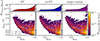 |
Fig. 5. Probability density of massive contact binaries in (qobs, pobs) (lower panels) and qobs space (upper panels) for our three model grids. The thin black lines are HDIs of the indicated percentiles. The parameters of observed systems from the Milky Way (MW) and Magellanic Clouds (MC) are listed in Tables D.1 and D.2. |
 |
Fig. 6. Cumulative distributions as function of observed mass ratio for the full synthetic populations (full lines), the populations considering only masses above 20 M⊙ (dashed lines), and the observed sample of Tables D.1 and D.2 (gray line). |
Kolmogorov-Smirnov (KS) tests of the observed sample (Tables D.2 and D.1) with respect to the ET, no-ET, and single-rotation model distributions give p values of 6.2 × 10⁻⁸, 7.3 × 10⁻⁸, and 4.8 × 10⁻⁷, respectively, indicating that it is extremely unlikely that these distributions correctly represent the observed sample.
Because the observed systems heavily favor massive O+O contact binaries, in Fig. 6 we also plot the CDFs when considering only the models with an initial primary mass higher than 20 M⊙ (dashed lines). We note that all grids of models are less clustered toward mass ratios of unity; however, despite the shift in the right direction, we still over-predict mass ratios close to unity. Performing a KS test on the ET models with a mass of M1,init > 20 M⊙ returns a p value of 0.003, indicating that, unless we require a confidence level higher than 99.7%, we can conclude that the current observed sample is not distributed according to the models. A KS test on the no-ET and high-mass, single-rotating models gives p values of only 1 × 10⁻⁴ and 5 × 10⁻⁴, respectively.
3.3. Luminosity ratios
Despite not significantly affecting the mass-ratio evolution of massive contact binaries, ET does affect other observable properties of the models. Since ET raises the luminosity of the energy gainer and reduces it for the energy donor, we expect a significantly different luminosity ratio of models in contact that include ET versus those that do not.
In Fig. 7, we plot the probability density as function of the observed mass and luminosity ratio of the whole population. We see a very clear difference between the model distributions that apply ET (left panel) and those that do not (two rightmost panels). When ET is applied, the models follow a L ∼ q relation closely, as expected from the theory discussed in Paper II. The no-ET and single-rotating models instead follow the single-star mass-luminosity relation L ∼ q2.5. We refrain from making a formal comparison with the observed sample because it could be contaminated with shallow-contact and near-contact systems. This is important because for the luminosity ratio to follow a L ∼ q relation, there must be good thermal contact between the components, which might not be the case for shallow contact systems (Paper II, Sect. 4.4); this is precluded for (semi-)detached ones.
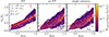 |
Fig. 7. Probability densities in observed mass- and luminosity-ratio space. L2/L1 means the ratio of the luminosity of the less massive star to that of the more massive star. We observe a clear difference in the model distributions when ET is applied. |
3.4. Observational biases in the sample
The KS tests performed above indicate that, from a statistical point of view, we must reject the hypothesis that the observational sample is distributed per our model distributions. Still, there could be observational biases that skew the sample. It could be that the sample of contact binaries is heavily biased toward detecting unequal-mass systems. However, owing to their short periods and large radial-velocity semi-amplitudes, all systems, regardless of mass ratio, should be picked up in long-term spectroscopic monitoring programs (such as VFTS, Evans et al. 2011; and TMBM, Almeida et al. 2017). Photometric characterization is not dependent on mass ratio either. There thus seem to be no obvious observational biases in terms of mass ratio in the current sample of massive contact binaries, apart from its completeness. In terms of primary mass, however, the characterization of individual systems seems biased toward higher masses. From Tables D.1 and D.2, the amount of O+O binaries that were studied far outnumbers the B+B contact systems when compared to a Salpeter IMF. Comparing the observational sample to models that reach down to initial primary masses of 8 M⊙ might thus skew the results, since the sample contains an under-represented number of B+B contact binaries compared to the distribution used in the population modeling. Still, limiting our population to systems with a primary mass higher than 20 M⊙ makes only a small improvement, as shown in Fig. 6. Finally, we note that the current sample of observed contact binaries is a very heterogeneous set, where many different observations and analysis tools were used. This makes it hard to discern the true contact binaries from those that are only near contact ones. Menon et al. (2024) homogeneously studied 61 contact-binary candidates in the Magellanic Clouds, which, combined with spectroscopic follow-up and advanced analysis methods as in Abdul-Masih et al. (2021), would significantly improve the quality of the sample.
3.5. Uncertain population distributions
A final consideration is the initial period distribution of binaries. Taking into account the indications that binaries harden over nuclear timescales (Sana et al. 2017; Ramírez-Tannus et al. 2021, 2024), the true ZAMS period distribution potentially does not follow an Öpik-like law down to periods of one day. We might even have to consider alternative initial conditions, where one star is at the ZAMS, while the other is still on the PMS. This would require putting in place new modeling efforts, whereby the star formation process and the potential interaction with its natal environment on the orbital evolution are included.
With the models computed in this work, we can, however, test the following. As we did above by considering very high-mass stars alone, here we test whether imposing a low-period cut on the ZAMS period distributions reconciles the models with the observations. In practice, this means we prevent the systems that interact on the ZAMS (or early on the main sequence) from contributing to the population predictions, effectively restricting the population to Classes II, III, and IV.
In Fig. 9, we show the KS-test p values when imposing different short-period cutoffs pcut. We emphasize that this means that the birth distribution probability density is Öpik’s law (Eq. 8c) down to pcut, but zero for pinit ≤ pcut. We see that the population predictions of contact binaries are very sensitive to the assumed birth distribution. At pcut = 1.26 d, the KS statistic of the mass-ratio distribution reaches a minimum of 0.15 for the ET-models, while it is 0.18 for both the no-ET and single-rotating models. This corresponds to p-values of 0.53 and 0.30, respectively, indicating that, to a high level of confidence, we cannot reject the hypothesis that the observed sample is drawn from the distribution with this period cut. Figure 10 shows the corresponding cumulative probability distributions and points out that the models now overestimate the extreme-mass-ratio contact binaries. We note, however, that by placing this cut we cannot explain the period distribution of the sample (see Fig. 8). This result suggests that systems with periods of p ≲ pcut at the ZAMS might not occur in nature, and instead might have merged before we observe them. Making concrete statements, however, would require an in-depth study of the impact of including alternate ZAMS conditions in a population, and these should include potential interactions with the star-formation environment.
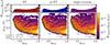 |
Fig. 8. Probability density distribution in (qobs, pobs) space for population with pcut = 1.26 d. With this period cut, we cannot predict the contact binaries with periods of p ≲ 1.2 d. |
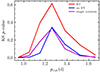 |
Fig. 9. KS-test p values when comparing empirical CDF of observed sample of massive contact binaries (Tables D.1 and D.2) against Öpik initial period distributions with a low-period cutoff pcut. |
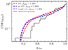 |
Fig. 10. CDFs of population as function of observed mass ratio using the low-period cutoff pcut = 1.26 d. From the KS statistic (Fig. 9), the observed sample is most likely drawn from the birth distribution with this value for pcut. |
4. Conclusions
In this work, we computed Case A interacting binary models and constructed synthetic populations of short-period, massive binary systems. We find that the inclusion of the effect of efficient ET in the shared envelopes of contact binaries does not fully reconcile the model predictions with the observed sample, in particular on their mass-ratio distribution. Many of the models avoid nuclear-timescale contact phases (those of Class III in Sect. 3.1), or enter contact so early on the main sequence that they equalize in mass within a thermal timescale (Class I) regardless of whether ET is applied or not. ET only has a significant effect on a small fraction of the models (Class II), where the equalization is delayed as ET modifies the internal structure of the components. The energy gainer bloats, while the energy donor shrinks, slightly altering the mass-radius relationship, which impacts whether a thermally stable contact configuration is possible. However, the combination of nuclear evolution and efficient rejuvenation of the stellar cores due to overshooting results in the mass ratio evolving to values of unity reasonably quickly.
From these points, we conclude that unequal-mass contact binaries must be reasonably evolved systems. More specifically, at least one of the components must be significantly departed from the ZAMS for its mass-radius relationship to be closer to that of the Roche-lobe geometry. Rejuvenation of the accretor during MT events might not be as efficient as that modeled here (Braun & Langer 1995), and this likely impacts the results. In Förster (2023), it is shown that changing the near-core mixing properties, such as the overshooting strength, semi-convective efficiency, and convective penetration of molecular weight barriers, can have a significant effect on the evolution of contact binaries. Near-core mixing properties of massive stars are uncertain, but asteroseismic analysis can probe the near-core region, and constrain, for example, overshooting parameters (e.g., Pedersen et al. 2021; Michielsen et al. 2021; Burssens et al. 2023; Johnston et al. 2024; Bellinger et al. 2024). Recently, it has been identified that stellar mergers, which have different internal mixing properties than genuine single stars, should reveal clear asteroseismic signatures (Henneco et al. 2024b).
We find indications that contact-binary progenitors could be affected by orbital hardening over their lifetimes. First, our models show that the very short-period binaries that interact early on the main sequence (when the stars are still relatively homogeneous) do not form contact binaries of unequal mass. Since we observe a fair number of such unequal systems, this suggests the closest binaries, which predominantly form equal-mass contact binaries, merge before being observed or even before they reach the ZAMS (as the Class 0 models). Secondly, when we restricted our population to models of Classes II and III only, we better fit the observed mass-ratio distribution. This suggests that the initial-period population could be distributed to somewhat longer periods, allowing time for the components to evolve from the ZAMS, and shrink on the nuclear timescale to become the contact binaries we observe today. Both these points indicate that the initial period distribution (at the ZAMS) is likely not Öpik’s law down to periods shorter than p ≲ 2 d. Further models of massive binaries, which allow for interaction on the PMS and/or include a prescription for orbital perturbations by the natal environment, are necessary to study this.
Finally, we advocate for renewed efforts to characterize massive contact binaries. Not only is the sample size rather limited, it is also heterogeneous. In order to achieve a comprehensive sample of confirmed contact binaries, studies similar to that of Menon et al. (2024) should be undertaken and followed up with homogeneous spectroscopic analyses such as Abdul-Masih et al. (2021) to clearly distinguish the near-contact binaries from the true contact ones. The modeling of massive contact binaries, from this work or in Menon et al. (2021, 2024), has reached a good level, and we are currently limited by observational constraints on contact binaries to further unravel their evolution.
Data availability
All input files and scripts required to reproduce the results of this work are made available on Zenodo at https://doi.org/10.5281/zenodo.14630181
Acknowledgments
M.F. thanks the Flemish research foundation (FWO, Fonds voor Wetenschappelijk Onderzoek) PhD fellowship No. 11H2421N for its support. P.M. acknowledges support from the FWO senior postdoctoral fellowship No. 12ZY523N. This work has made use of the computing resources of the Vlaams Supercomputer Center (VSC), funded by the FWO. The research leading to these results has received funding from the European Research Council (ERC) under the European Union’s Horizon 2020 research and innovation program (grant agreement numbers 772225: MULTIPLES). Data processing and visualization has been made possible thanks to matplotlib (Hunter 2007), scipy (Virtanen et al. 2020) and numpy (Harris et al. 2020).
References
- Abdul-Masih, M., Sana, H., Conroy, K. E., et al. 2020, A&A, 636, A59 [NASA ADS] [CrossRef] [EDP Sciences] [Google Scholar]
- Abdul-Masih, M., Sana, H., Hawcroft, C., et al. 2021, A&A, 651, A96 [NASA ADS] [CrossRef] [EDP Sciences] [Google Scholar]
- Abdul-Masih, M., Escorza, A., Menon, A., Mahy, L., & Marchant, P. 2022, A&A, 666, A18 [NASA ADS] [CrossRef] [EDP Sciences] [Google Scholar]
- Aguilera-Dena, D. R., Langer, N., Moriya, T. J., & Schootemeijer, A. 2018, ApJ, 858, 115 [NASA ADS] [CrossRef] [Google Scholar]
- Aguilera-Dena, D. R., Langer, N., Antoniadis, J., & Müller, B. 2020, ApJ, 901, 114 [NASA ADS] [CrossRef] [Google Scholar]
- Alcock, C., Allsman, R. A., Alves, D., et al. 1997, AJ, 114, 326 [NASA ADS] [CrossRef] [Google Scholar]
- Almeida, L. A., Sana, H., de Mink, S. E., et al. 2015, ApJ, 812, 102 [Google Scholar]
- Almeida, L. A., Sana, H., Taylor, W., et al. 2017, A&A, 598, A84 [NASA ADS] [CrossRef] [EDP Sciences] [Google Scholar]
- Anderson, L., & Shu, F. H. 1977, ApJ, 214, 798 [NASA ADS] [CrossRef] [Google Scholar]
- Angulo, C., Arnould, M., Rayet, M., et al. 1999, Nucl. Phys. A, 656, 3 [Google Scholar]
- Asplund, M., Grevesse, N., Sauval, A. J., & Scott, P. 2009, ARA&A, 47, 481 [NASA ADS] [CrossRef] [Google Scholar]
- Banyard, G., Sana, H., Mahy, L., et al. 2022, A&A, 658, A69 [NASA ADS] [CrossRef] [EDP Sciences] [Google Scholar]
- Bastian, N., Covey, K. R., & Meyer, M. R. 2010, ARA&A, 48, 339 [Google Scholar]
- Bellinger, E. P., de Mink, S. E., van Rossem, W. E., & Justham, S. 2024, ApJ, 967, L39 [NASA ADS] [CrossRef] [Google Scholar]
- Biermann, P., & Thomas, H. C. 1972, A&A, 16, 60 [NASA ADS] [Google Scholar]
- Binnendijk, L. 1970, Vistas Astron., 12, 217 [NASA ADS] [CrossRef] [Google Scholar]
- Blouin, S., Shaffer, N. R., Saumon, D., & Starrett, C. E. 2020, ApJ, 899, 46 [NASA ADS] [CrossRef] [Google Scholar]
- Bodensteiner, J., Heida, M., Abdul-Masih, M., et al. 2022, The Messenger, 186, 3 [NASA ADS] [Google Scholar]
- Böhm-Vitense, E. 1958, Zeit. Astro., 46, 108 [Google Scholar]
- Bondi, H., & Hoyle, F. 1944, MNRAS, 104, 273 [Google Scholar]
- Braun, H., & Langer, N. 1995, A&A, 297, 483 [NASA ADS] [Google Scholar]
- Brott, I., de Mink, S. E., Cantiello, M., et al. 2011, A&A, 530, A115 [NASA ADS] [CrossRef] [EDP Sciences] [Google Scholar]
- Burssens, S., Bowman, D. M., Michielsen, M., et al. 2023, Nat. Astron., 7, 913 [NASA ADS] [CrossRef] [Google Scholar]
- Çakırlı, Ö., Ibanoglu, C., & Sipahi, E. 2014, MNRAS, 442, 1560 [CrossRef] [Google Scholar]
- Cassisi, S., Potekhin, A. Y., Pietrinferni, A., Catelan, M., & Salaris, M. 2007, ApJ, 661, 1094 [NASA ADS] [CrossRef] [Google Scholar]
- Chugunov, A. I., Dewitt, H. E., & Yakovlev, D. G. 2007, Phys. Rev. D, 76, 025028 [NASA ADS] [CrossRef] [Google Scholar]
- Cox, J. P., & Giuli, R. T. 1968, Principles of Stellar Structure (New York: Gordon and Breach) [Google Scholar]
- Cyburt, R. H., Amthor, A. M., Ferguson, R., et al. 2010, ApJS, 189, 240 [NASA ADS] [CrossRef] [Google Scholar]
- Darwin, G. H. 1879, Proc. Roy. Soc. London, 29, 168 [NASA ADS] [CrossRef] [Google Scholar]
- de Mink, S. E., Langer, N., Izzard, R. G., Sana, H., & de Koter, A. 2013, ApJ, 764, 166 [Google Scholar]
- Drout, M. R., Götberg, Y., Ludwig, B. A., et al. 2023, Science, 382, 1287 [NASA ADS] [CrossRef] [Google Scholar]
- Dunstall, P. R., Dufton, P. L., Sana, H., et al. 2015, A&A, 580, A93 [NASA ADS] [CrossRef] [EDP Sciences] [Google Scholar]
- Eddington, A. S. 1925, The Observatory, 48, 73 [NASA ADS] [Google Scholar]
- Eggen, O. J. 1967, Mem. R. Astron. Soc., 70, 111 [NASA ADS] [Google Scholar]
- Eggleton, P. P. 1983, ApJ, 268, 368 [Google Scholar]
- Endal, A. S., & Sofia, S. 1978, ApJ, 220, 279 [NASA ADS] [CrossRef] [Google Scholar]
- Evans, C. J., Taylor, W. D., Hénault-Brunet, V., et al. 2011, A&A, 530, A108 [NASA ADS] [CrossRef] [EDP Sciences] [Google Scholar]
- Fabry, M., Marchant, P., & Sana, H. 2022, A&A, 661, A123 [NASA ADS] [CrossRef] [EDP Sciences] [Google Scholar]
- Fabry, M., Marchant, P., Langer, N., & Sana, H. 2023, A&A, 672, A175 [NASA ADS] [CrossRef] [EDP Sciences] [Google Scholar]
- Ferguson, J. W., Alexander, D. R., Allard, F., et al. 2005, ApJ, 623, 585 [Google Scholar]
- Flannery, B. P. 1976, ApJ, 205, 217 [NASA ADS] [CrossRef] [Google Scholar]
- Förster, K. U. 2023, Evolution of Massive Contact Binaries, https://astro.uni-bonn.de/ nlanger/thesis/kai_bachelor.pdf [Google Scholar]
- Fricke, K. 1968, Zeit. Astro., 68, 317 [NASA ADS] [Google Scholar]
- Frost, A. J., Sana, H., Mahy, L., et al. 2024, Science, 384, 214 [NASA ADS] [CrossRef] [Google Scholar]
- Fuller, G. M., Fowler, W. A., & Newman, M. J. 1985, ApJ, 293, 1 [NASA ADS] [CrossRef] [Google Scholar]
- Goldreich, P., & Schubert, G. 1967, ApJ, 150, 571 [Google Scholar]
- Graczyk, D., Soszyński, I., Poleski, R., et al. 2011, Acta Astron., 61, 103 [Google Scholar]
- Graczyk, D., Pietrzyński, G., Thompson, I. B., et al. 2018, ApJ, 860, 1 [NASA ADS] [CrossRef] [Google Scholar]
- Guo, Y., Li, J., Xiong, J., et al. 2022, Res. Astron. Astrophys., 22, 025009 [CrossRef] [Google Scholar]
- Hainich, R., Rühling, U., Todt, H., et al. 2014, A&A, 565, A27 [NASA ADS] [CrossRef] [EDP Sciences] [Google Scholar]
- Hamann, W.-R., Koesterke, L., & Wessolowski, U. 1995, A&A, 299, 151 [NASA ADS] [Google Scholar]
- Harris, C. R., Millman, K. J., van der Walt, S. J., et al. 2020, Nature, 585, 357 [NASA ADS] [CrossRef] [Google Scholar]
- Hazlehurst, J. 1993, A&A, 271, 209 [NASA ADS] [Google Scholar]
- Hazlehurst, J., & Refsdal, S. 1980, A&A, 84, 200 [NASA ADS] [Google Scholar]
- Heger, A., Langer, N., & Woosley, S. E. 2000, ApJ, 528, 368 [NASA ADS] [CrossRef] [Google Scholar]
- Henneco, J., Schneider, F. R. N., & Laplace, E. 2024a, A&A, 682, A169 [NASA ADS] [CrossRef] [EDP Sciences] [Google Scholar]
- Henneco, J., Schneider, F. R. N., Hekker, S., & Aerts, C. 2024b, A&A, 690, A65 [NASA ADS] [CrossRef] [EDP Sciences] [Google Scholar]
- Hilditch, R. W., & Evans, T. L. 1985, MNRAS, 213, 75 [CrossRef] [Google Scholar]
- Hilditch, R. W., Howarth, I. D., & Harries, T. J. 2005, MNRAS, 357, 304 [NASA ADS] [CrossRef] [Google Scholar]
- Hunter, J. D. 2007, Comput. Sci. Eng., 9, 90 [NASA ADS] [CrossRef] [Google Scholar]
- Hurley, J. R., Tout, C. A., & Pols, O. R. 2002, MNRAS, 329, 897 [Google Scholar]
- Iglesias, C. A., & Rogers, F. J. 1993, ApJ, 412, 752 [Google Scholar]
- Iglesias, C. A., & Rogers, F. J. 1996, ApJ, 464, 943 [NASA ADS] [CrossRef] [Google Scholar]
- Itoh, N., Hayashi, H., Nishikawa, A., & Kohyama, Y. 1996, ApJS, 102, 411 [NASA ADS] [CrossRef] [Google Scholar]
- Jermyn, A. S., Schwab, J., Bauer, E., Timmes, F. X., & Potekhin, A. Y. 2021, ApJ, 913, 72 [NASA ADS] [CrossRef] [Google Scholar]
- Jermyn, A. S., Bauer, E. B., Schwab, J., et al. 2023, ApJS, 265, 15 [NASA ADS] [CrossRef] [Google Scholar]
- Johnston, C., Michielsen, M., Anders, E. H., et al. 2024, ApJ, 964, 170 [NASA ADS] [Google Scholar]
- Kähler, H. 1989, A&A, 209, 67 [NASA ADS] [Google Scholar]
- Kippenhahn, R., Ruschenplatt, G., & Thomas, H. C. 1980, A&A, 91, 175 [Google Scholar]
- Kobulnicky, H. A., Kiminki, D. C., Lundquist, M. J., et al. 2014, ApJS, 213, 34 [Google Scholar]
- Kroupa, P. 2001, MNRAS, 322, 231 [NASA ADS] [CrossRef] [Google Scholar]
- Kuiper, G. P. 1941, ApJ, 93, 133 [NASA ADS] [CrossRef] [Google Scholar]
- Langanke, K., & Martínez-Pinedo, G. 2000, Nucl. Phys. A, 673, 481 [NASA ADS] [CrossRef] [Google Scholar]
- Langer, N., Fricke, K. J., & Sugimoto, D. 1983, A&A, 126, 207 [NASA ADS] [Google Scholar]
- Lanthermann, C., Le Bouquin, J. B., Sana, H., et al. 2023, A&A, 672, A6 [NASA ADS] [CrossRef] [EDP Sciences] [Google Scholar]
- Ledoux, P. 1947, ApJ, 105, 305 [NASA ADS] [CrossRef] [Google Scholar]
- Leung, K. C., Sistero, R. F., Zhai, D. S., Grieco, A., & Candellero, B. 1984, AJ, 89, 872 [NASA ADS] [CrossRef] [Google Scholar]
- Li, L., & Zhang, F. 2006, MNRAS, 369, 2001 [CrossRef] [Google Scholar]
- Li, L., Han, Z., & Zhang, F. 2004, MNRAS, 355, 1383 [NASA ADS] [CrossRef] [Google Scholar]
- Li, L., Han, Z., & Zhang, F. 2005, MNRAS, 360, 272 [NASA ADS] [CrossRef] [Google Scholar]
- Li, F. X., Liao, W. P., Qian, S. B., et al. 2022a, ApJ, 924, 30 [NASA ADS] [CrossRef] [Google Scholar]
- Li, F. X., Qian, S. B., Jiao, C. L., & Ma, W. W. 2022b, ApJ, 932, 14 [NASA ADS] [CrossRef] [Google Scholar]
- Linnell, A. P., & Scheick, X. 1991, ApJ, 379, 721 [NASA ADS] [CrossRef] [Google Scholar]
- Lorenz, R., Mayer, P., & Drechsel, H. 1999, A&A, 345, 531 [NASA ADS] [Google Scholar]
- Lorenzo, J., Negueruela, I., Baker, A. K. F. V., et al. 2014, A&A, 572, A110 [NASA ADS] [CrossRef] [EDP Sciences] [Google Scholar]
- Lorenzo, J., Simón-Díaz, S., Negueruela, I., et al. 2017, A&A, 606, A54 [NASA ADS] [CrossRef] [EDP Sciences] [Google Scholar]
- Lucy, L. B. 1967, Zeit. Astro., 65, 89 [NASA ADS] [Google Scholar]
- Lucy, L. B. 1968, ApJ, 151, 1123 [Google Scholar]
- Lucy, L. B. 1976, ApJ, 205, 208 [NASA ADS] [CrossRef] [Google Scholar]
- Mahy, L., Almeida, L. A., Sana, H., et al. 2020a, A&A, 634, A119 [NASA ADS] [CrossRef] [EDP Sciences] [Google Scholar]
- Mahy, L., Sana, H., Abdul-Masih, M., et al. 2020b, A&A, 634, A118 [NASA ADS] [CrossRef] [EDP Sciences] [Google Scholar]
- Mandel, I., & de Mink, S. E. 2016, MNRAS, 458, 2634 [NASA ADS] [CrossRef] [Google Scholar]
- Marchant, P., & Bodensteiner, J. 2024, ARA&A, 62, 21 [NASA ADS] [CrossRef] [Google Scholar]
- Marchant, P., Langer, N., Podsiadlowski, P., Tauris, T. M., & Moriya, T. J. 2016, A&A, 588, A50 [NASA ADS] [CrossRef] [EDP Sciences] [Google Scholar]
- Martins, F., Mahy, L., & Hervé, A. 2017, A&A, 607, A82 [NASA ADS] [CrossRef] [EDP Sciences] [Google Scholar]
- Mason, B. D., Hartkopf, W. I., Gies, D. R., Henry, T. J., & Helsel, J. W. 2009, AJ, 137, 3358 [Google Scholar]
- Mayer, P., Drechsel, H., Harmanec, P., Yang, S., & Šlechta, M. 2013, A&A, 559, A22 [NASA ADS] [CrossRef] [EDP Sciences] [Google Scholar]
- Menon, A., Langer, N., de Mink, S. E., et al. 2021, MNRAS, 507, 5013 [NASA ADS] [CrossRef] [Google Scholar]
- Menon, A., Pawlak, M., Lennon, D. J., Sen, K., & Langer, N. 2024, ArXiv e-prints [arXiv:2410.16427] [Google Scholar]
- Michielsen, M., Aerts, C., & Bowman, D. M. 2021, A&A, 650, A175 [NASA ADS] [CrossRef] [EDP Sciences] [Google Scholar]
- Moe, M., & Di Stefano, R. 2017, ApJS, 230, 15 [Google Scholar]
- Nelson, C. A., & Eggleton, P. P. 2001, ApJ, 552, 664 [NASA ADS] [CrossRef] [Google Scholar]
- Nieuwenhuijzen, H., & de Jager, C. 1995, A&A, 302, 811 [NASA ADS] [Google Scholar]
- Oda, T., Hino, M., Muto, K., Takahara, M., & Sato, K. 1994, At. Data Nucl. Data Tables, 56, 231 [NASA ADS] [CrossRef] [Google Scholar]
- Öpik, E. 1924, Publications of the Tartu Astrofizica Observatory, 25, 1 [Google Scholar]
- Ostrov, P. G. 2001, MNRAS, 321, L25 [NASA ADS] [CrossRef] [Google Scholar]
- Paczynski, B., Szczygiel, D., Pilecki, B., & Pojmanski, G. 2006, MNRAS, 368, 1311 [CrossRef] [Google Scholar]
- Papaloizou, J., & Pringle, J. E. 1979, MNRAS, 189, 5P [NASA ADS] [CrossRef] [Google Scholar]
- Pauli, D., Langer, N., Aguilera-Dena, D. R., Wang, C., & Marchant, P. 2022, A&A, 667, A58 [NASA ADS] [CrossRef] [EDP Sciences] [Google Scholar]
- Paxton, B., Bildsten, L., Dotter, A., et al. 2011, ApJS, 192, 3 [Google Scholar]
- Paxton, B., Cantiello, M., Arras, P., et al. 2013, ApJS, 208, 4 [Google Scholar]
- Paxton, B., Marchant, P., Schwab, J., et al. 2015, ApJS, 220, 15 [Google Scholar]
- Paxton, B., Schwab, J., Bauer, E. B., et al. 2018, ApJS, 234, 34 [NASA ADS] [CrossRef] [Google Scholar]
- Paxton, B., Smolec, R., Schwab, J., et al. 2019, ApJS, 243, 10 [Google Scholar]
- Pedersen, M. G., Aerts, C., Pápics, P. I., et al. 2021, Nat. Astron., 5, 715 [NASA ADS] [CrossRef] [Google Scholar]
- Pejcha, O. 2014, ApJ, 788, 22 [NASA ADS] [CrossRef] [Google Scholar]
- Penny, L. R., Ouzts, C., & Gies, D. R. 2008, ApJ, 681, 554 [Google Scholar]
- Podsiadlowski, P., Rappaport, S., & Pfahl, E. D. 2002, ApJ, 565, 1107 [NASA ADS] [CrossRef] [Google Scholar]
- Pols, O. R. 1994, A&A, 290, 119 [Google Scholar]
- Polushina, T. S. 2004, Astron. Astrophys. Trans., 23, 213 [NASA ADS] [CrossRef] [Google Scholar]
- Potekhin, A. Y., & Chabrier, G. 2010, Contrib. Plasma Phys., 50, 82 [NASA ADS] [CrossRef] [Google Scholar]
- Poutanen, J. 2017, ApJ, 835, 119 [NASA ADS] [CrossRef] [Google Scholar]
- Ramírez-Tannus, M. C., Backs, F., de Koter, A., et al. 2021, A&A, 645, L10 [NASA ADS] [CrossRef] [EDP Sciences] [Google Scholar]
- Ramírez-Tannus, M. C., Derkink, A. R., Backs, F., et al. 2024, A&A, 690, A178 [NASA ADS] [CrossRef] [EDP Sciences] [Google Scholar]
- Rasio, F. A. 1995, ApJ, 444, L41 [NASA ADS] [CrossRef] [Google Scholar]
- Raucq, F., Gosset, E., Rauw, G., et al. 2017, A&A, 601, A133 [NASA ADS] [CrossRef] [EDP Sciences] [Google Scholar]
- Rogers, F. J., & Nayfonov, A. 2002, ApJ, 576, 1064 [Google Scholar]
- Salpeter, E. E. 1955, ApJ, 121, 161 [Google Scholar]
- Sana, H., de Mink, S. E., de Koter, A., et al. 2012, Science, 337, 444 [Google Scholar]
- Sana, H., de Koter, A., de Mink, S. E., et al. 2013, A&A, 550, A107 [NASA ADS] [CrossRef] [EDP Sciences] [Google Scholar]
- Sana, H., Le Bouquin, J. B., Lacour, S., et al. 2014, ApJS, 215, 15 [Google Scholar]
- Sana, H., Ramírez-Tannus, M. C., de Koter, A., et al. 2017, A&A, 599, L9 [NASA ADS] [CrossRef] [EDP Sciences] [Google Scholar]
- Saumon, D., Chabrier, G., & van Horn, H. M. 1995, ApJS, 99, 713 [NASA ADS] [CrossRef] [Google Scholar]
- Schneider, F. R. N., Ohlmann, S. T., Podsiadlowski, P., et al. 2019, Nature, 574, 211 [Google Scholar]
- Selam, S. O. 2004, A&A, 416, 1097 [NASA ADS] [CrossRef] [EDP Sciences] [Google Scholar]
- Sen, K., Langer, N., Marchant, P., et al. 2022, A&A, 659, A98 [NASA ADS] [CrossRef] [EDP Sciences] [Google Scholar]
- Shenar, T., Bodensteiner, J., Abdul-Masih, M., et al. 2020, A&A, 639, L6 [EDP Sciences] [Google Scholar]
- Shenar, T., Sana, H., Mahy, L., et al. 2022, A&A, 665, A148 [NASA ADS] [CrossRef] [EDP Sciences] [Google Scholar]
- Shu, F. H., Lubow, S. H., & Anderson, L. 1976, ApJ, 209, 536 [NASA ADS] [CrossRef] [Google Scholar]
- Shu, F. H., Lubow, S. H., & Anderson, L. 1979, ApJ, 229, 223 [NASA ADS] [CrossRef] [Google Scholar]
- Sills, A., Pinsonneault, M. H., & Terndrup, D. M. 2000, ApJ, 534, 335 [NASA ADS] [CrossRef] [Google Scholar]
- Stȩpień, K. 2009, MNRAS, 397, 857 [CrossRef] [Google Scholar]
- Sweet, P. A. 1950, MNRAS, 110, 548 [Google Scholar]
- Szymanski, M., Kubiak, M., & Udalski, A. 2001, Acta Astron., 51, 259 [NASA ADS] [Google Scholar]
- Timmes, F. X., & Swesty, F. D. 2000, ApJS, 126, 501 [NASA ADS] [CrossRef] [Google Scholar]
- Tokovinin, A., & Moe, M. 2020, MNRAS, 491, 5158 [NASA ADS] [CrossRef] [Google Scholar]
- Vanbeveren, D., De Donder, E., Van Bever, J., Van Rensbergen, W., & De Loore, C. 1998, New Astron., 3, 443 [CrossRef] [Google Scholar]
- Villaseñor, J. I., Taylor, W. D., Evans, C. J., et al. 2021, MNRAS, 507, 5348 [CrossRef] [Google Scholar]
- Vink, J. S., de Koter, A., & Lamers, H. J. G. L. M. 2001, A&A, 369, 574 [NASA ADS] [CrossRef] [EDP Sciences] [Google Scholar]
- Virtanen, P., Gommers, R., Oliphant, T. E., et al. 2020, Nat. Meth., 17, 261 [Google Scholar]
- Vitense, E. 1953, Zeit. Astro., 32, 135 [NASA ADS] [Google Scholar]
- von Zeipel, H. 1924, MNRAS, 84, 665 [NASA ADS] [CrossRef] [Google Scholar]
- Vrancken, J., Abdul-Masih, M., Escorza, A., et al. 2024, A&A, 691, A150 [NASA ADS] [CrossRef] [EDP Sciences] [Google Scholar]
- Wellstein, S., Langer, N., & Braun, H. 2001, A&A, 369, 939 [NASA ADS] [CrossRef] [EDP Sciences] [Google Scholar]
- Wilson, R. E., & Devinney, E. J. 1971, ApJ, 166, 605 [Google Scholar]
- Yakut, K., & Eggleton, P. P. 2005, ApJ, 629, 1055 [NASA ADS] [CrossRef] [Google Scholar]
- Yang, Y., Yuan, H., & Dai, H. 2019, AJ, 157, 111 [NASA ADS] [CrossRef] [Google Scholar]
- Yaşarsoy, B., & Yakut, K. 2014, New Astron., 31, 32 [CrossRef] [Google Scholar]
- Yoon, S. C., & Langer, N. 2005, A&A, 443, 643 [NASA ADS] [CrossRef] [EDP Sciences] [Google Scholar]
- Yoon, S.-C., Langer, N., & Norman, C. 2006, A&A, 460, 199 [NASA ADS] [CrossRef] [EDP Sciences] [Google Scholar]
- Zahn, J.-P. 1975, A&A, 41, 329 [Google Scholar]
- Zahn, J.-P. 1977, A&A, 500, 121 [Google Scholar]
- Zahn, J.-P. 1992, A&A, 265, 115 [NASA ADS] [Google Scholar]
- Zhou, D.-Q., & Leung, K.-C. 1990, ApJ, 355, 271 [NASA ADS] [CrossRef] [Google Scholar]
Appendix A: Roche-lobe overflow at the zero-age main sequence
In this appendix we discuss the models that experience RLOF at the ZAMS. We expect these systems to strongly interact on the PMS, and to account for this possibility, we perform an artificial shrinking of the orbit toward their initial period. We model these systems as follows.
We start with the model at ZAMS as described in Sect. 2.2. In the case considered here, the more massive star will overflow the RL (potentially by a large amount since we ignore MT in the relaxation phase). We then artificially modify the orbital period to put the components in a detached configuration, adding a certain amount of angular momentum to the orbit. Finally, on a thermal timescale of the more massive star (τ = 0.75GM12/R1L1), we drain the added angular momentum from the system to again reach the initial period, while allowing MT and ET. This process allows the models to smoothly start RLOF, and is more of a technical modification to the models instead of being physically motivated. A more accurate model would be to follow the evolution of forming massive stars throughout the PMS, and include some prescription of angular momentum loss through interaction with a disk or their natal cloud, but this is beyond the scope of this work.
A.1. Results
Figure A.1 shows the orbital period and mass-ratio evolution of the 20 M⊙ model with initial mass ratio of q = 0.8 and initial periods between 0.8 − 1.05 day. Note the logarithmic scale on the x-axis. The models reach our definition of the ZAMS at around 0.02 Myr, after which we boost the period and initiate the shrinking on the thermal timescale of the primary.
We emphasize that we do not treat the shrinking process fully. Sana et al. (2017) analyzed the RV-dispersion of young stars in M17, and inferred that the underlying period distribution fits best if there is a short-period cutoff at p ≈ 50 d. Presumably then, the stars start their migration inward toward a distribution that follows an Öpik-like law, Eq. (8c), down to periods of around 1 d. Our toy migration model thus only covers the final 1% of the migration into a RL filling configuration (from ∼1.2 d to ≲1 d). It is however uncertain how, and on what timescale, migration happens, but the RV-dispersion analysis of Ramírez-Tannus et al. (2021) suggests it might be on the Myr nuclear timescale of massive stars. Therefore, there is a possibility that short-period binaries evolve significantly before they are observed as ∼1 d contact binaries. In contrast, we operate the shrinking on a (short) thermal timescale, so that the two stellar models do not have time to build a significant composition difference before they enter contact.
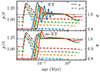 |
Fig. A.1. Period and mass-ratio evolution of the M1,init = 20 M⊙ models with qinit = 0.8 that experience RLOF at the ZAMS. The initial period of these models can be read off from the intersection with the left y-axis. All models interact before reaching their assumed initial period, meaning strong interaction on the PMS is expected. |
During the shrinking process, all models start MT before they reach their initial period again, signaling that significant interaction on the PMS could be important for very short-period binary systems. We note that, with or without ET, all models equalize to mass ratios close to unity within the first 0.1 Myr or so. The ET models show some oscillations because ET is actively regulating MT. In cases where the energy donor is the mass accretor, MT is invigorated, and this is generally the case in thermal-timescale MT events as the accretor gains significant luminosity as the accreted material thermally relaxes. Finally, it has not yet been unambiguously shown theoretically that homogeneous stellar models allow for a contact configuration with unequal masses. While Shu et al. (1979) argue for a thermally stable structure with a temperature inversion layer, Papaloizou & Pringle (1979) and Hazlehurst & Refsdal (1980) show this violates the second law of thermodynamics, and the discontinuity disappears within a thermal timescale. A model without such inconsistencies has not yet been presented. Since we chose to perform the tidal shrinking on the thermal timescale, preventing composition gradients from building, our (numerical) evolution models, with or without ET, indicate that a composition difference is needed to create stable contact binaries with mass ratios away from unity.
Despite some qualitative differences in their evolution, the ET and no-ET models show no significant difference in the mass-ratio distribution of contact binaries that experience RLOF at the ZAMS. From Figs. A.2 and A.3, we infer it is very unlikely to observe a contact binary that interacted on the PMS at mass ratios far from unity. From our models, there is only around a 1% chance a binary with a mass ratio more extreme than q = 0.8 will be observed. Conversely, over 95% of all PMS-interacting binaries should be observed with q > 0.95.
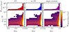 |
Fig. A.2. Probability density in (qobs, pobs) (lower panels) and qobs space (upper panels) for the models that experience RLOF at the ZAMS. The thin black lines are highest density intervals of the indicated percentiles, i.e., we expect to observe at most 3% of systems with a mass ratio significantly away from unity. |
Both observationally (Sana et al. 2017; Ramírez-Tannus et al. 2021, 2024) and theoretically (Tokovinin & Moe 2020), it has been suggested that hardening of binaries through disk migration is an ingredient in the formation of close binaries, such as contact-binary progenitors. Therefore, we think it fruitful to perform a population study of binaries with initial periods (on the PMS) of tens of days that harden over a Myr timescale.
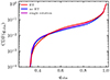 |
Fig. A.3. Cumulative probability distribution of the mass ratio of contact binaries that interact on the PMS. |
Appendix B: Width of the energy transfer layer
It was shown in Paper II that the thickness of the energy transferring layer might be underestimated at d = e − 2 RRL. Furthermore, in the low-mass contact binary regime, it is suggested that strong surface flows are the mechanism for energy transfer (e.g. Zhou & Leung 1990; Yakut & Eggleton 2005; Stȩpień 2009). It could thus be that in massive contact binaries, the energy flow likewise occurs across the entirety of the common layers.
For contact binaries evolving on the nuclear timescale, however, we note that the thermal timescale of the common layers is much shorter than the nuclear timescale of the stellar components. Therefore, the envelope has enough time to adjust to energy being transferred, and, to first order, it will not matter where precisely the energy is deposited, as long as the total amount is roughly the same. We show this in Fig. B.1, where we computed an equivalent model of Case II (Fig. 3), but we changed only the region of energy deposition to
 (B.1)
(B.1)
R being the (total) radius of the components, as opposed to 0.99RRL ≤ RET ≤ 1.01RRL in the default grid above. We see that, despite changing slightly the time at which nuclear timescale contact is engaged, the overall behavior of the model is unchanged, and we expect little difference in the population properties when using this ET prescription across the model grid. The slight time difference results from the fast MT phase, where contact is engaged in a thermal evolution regime, for which, by the same timescale argument, it does matter where energy is deposited.
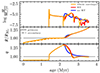 |
Fig. B.1. Evolution of the binary model with M1, init = 30 M⊙, pinit = 1.52 d, qinit = 0.9 (similar to Case II in Fig. 3), where we added the “whole envelope” model, which has ET occurring through the entirety of the common layers of the contact binary. |
Appendix C: Low-mass contact binary model
In this appendix we perform a computation of a low-mass, W UMa type contact binary, using the same modeling setup as presented in Sect. 2. To represent the solar-type stars and their interactions, the following modifications are made:
-
We model saturated magnetic braking as prescribed by Sills et al. (2000), with an envelope mass scaling following Podsiadlowski et al. (2002).
-
The amount of ET in convective envelopes is (nearly) independent of the local effective gravity (Lucy 1967; Anderson & Shu 1977), hence the luminosity of component 1 just above the RL is
 (C.1)
(C.1)with S the surface area of the RL of either component (cf. Eq. 8 of Paper II).
-
We turn off the step overshooting appropriate for convective cores of massive stars.
All other input physics, such as the microphysics, MT and rotation are the same.
In Fig. C.1, we show the MT rate, relative RL radii and the mass-evolution of the low-mass binary with initial parameters M1,init = 1.0 M⊙, pinit = 0.8 M⊙, qinit = 0.6. We see that over a Gyr timescale, the primary fills its RL as a result of angular momentum loss by magnetic braking. This initiates a Case A MT phase, which is interrupted when the secondary grows to its RL size, and the MT direction reverses. Then three thermal oscillation occur, where the system sequentially goes through detached and contact configurations. From the fourth oscillation on, there seems to be a marginally stable configuration at shallow overflow of (R − RRL/RRL ≈ 0.02), where the system evolves on the nuclear timescale of the primary. However, we expect the stability here to be sensitive to the precise implementation of ET, in particular its effective region (here modeled as 1% around the RL size, to stay similar to Sect. 2; see also Appendix B), and potential numerical smoothing (here 0.5, as in Paper II).
In the third right-hand panel of Fig. C.1, we see the mass ratio of the ET model evolving toward more extreme values. The black line shows the thermal timescale running average of the mass ratio
 (C.2)
(C.2)
with τKH ≈ 63 Myr, an estimation of the thermal timescale of the primary. We note also that without ET, no inflation and its associated inverse MT occurs, and the period of the system keeps decreasing until the model merges at mass ratio near unity. The contact phase in this case lasted less than 0.3 Gyr.
Our ET model calculated here behaves similarly to those of Li et al. (2004, 2005) and Yakut & Eggleton (2005). The late-time evolution of such models, as well as their properties at the onset of the merger, are yet unknown, but the Darwin instability (Darwin 1879; Rasio 1995; Li & Zhang 2006) or runaway MT by overflow of the L2 point (e.g. Pejcha 2014) are the primary mechanisms being considered.
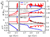 |
Fig. C.1. MT rate, radius, mass-ratio and period evolution of a low-mass contact binary model with and without ET. The right hand panels zoom in on the contact evolution, where thermal oscillations are present in the ET model. The no-ET model instead within 0.3 Gyr after first contact. The black line in the third right-hand panel shows the averaged mass ratio of the ET model, defined in Eq. (C.2). |
In future work, we will apply this modeling approach to a wider grid of low-mass contact binary systems, and investigate the impact of numerics, angular momentum loss prescriptions and ET prescriptions.
Appendix D: Observed systems
In this section we present the parameters from observed massive (near-)contact binaries in the Milky way and M31 (Table D.1) and the Magellanic Clouds (Table D.2). We took the period, mass ratio, masses, radii and temperatures from the indicated references, and computed R/RRL according to the approximation of Eggleton (1983) and Kepler’s third law. We note that in the Tables of Menon et al. (2021), some of their values, in particular on R/RRL, are misquoted.
Parameters of observed, massive (near-)contact systems in the Milky Way and M31.
Parameters of observed, massive (near-)contact systems in the Magellanic Clouds.
All Tables
Parameters of observed, massive (near-)contact systems in the Milky Way and M31.
Parameters of observed, massive (near-)contact systems in the Magellanic Clouds.
All Figures
|
Fig. 1. Termination conditions of 26 M⊙ and 62.5 M⊙ models that use ET as function of the initial mass ratio qinit = M2,init/M1,init and initial period pinit. In color we indicate the models that experience L2OF at the ZAMS (light blue), those that experience L2OF during the main sequence (orange, “mergers”) or experience a MT rate above 10−1 M⊙ yr−1 (dark blue), those that survive the main sequence without experiencing L2OF (yellow), and those terminate with a numerical error (red). Forward-hatched models experience contact during their main-sequence evolution, while backward-hatched models overflow their RL at the ZAMS. Outlined in white are five classes (“Class 0-IV”) of systems determined by their qualitative evolution (see Sect. 3.1). |
| In the text | |
|
Fig. 2. Evolution of a Class I system with initial parameters |
| In the text | |
|
Fig. 3. Evolution of a Class II system with initial parameters |
| In the text | |
|
Fig. 4. Evolution of a Class IV system with initial parameters |
| In the text | |
|
Fig. 5. Probability density of massive contact binaries in (qobs, pobs) (lower panels) and qobs space (upper panels) for our three model grids. The thin black lines are HDIs of the indicated percentiles. The parameters of observed systems from the Milky Way (MW) and Magellanic Clouds (MC) are listed in Tables D.1 and D.2. |
| In the text | |
|
Fig. 6. Cumulative distributions as function of observed mass ratio for the full synthetic populations (full lines), the populations considering only masses above 20 M⊙ (dashed lines), and the observed sample of Tables D.1 and D.2 (gray line). |
| In the text | |
|
Fig. 7. Probability densities in observed mass- and luminosity-ratio space. L2/L1 means the ratio of the luminosity of the less massive star to that of the more massive star. We observe a clear difference in the model distributions when ET is applied. |
| In the text | |
|
Fig. 8. Probability density distribution in (qobs, pobs) space for population with pcut = 1.26 d. With this period cut, we cannot predict the contact binaries with periods of p ≲ 1.2 d. |
| In the text | |
|
Fig. 9. KS-test p values when comparing empirical CDF of observed sample of massive contact binaries (Tables D.1 and D.2) against Öpik initial period distributions with a low-period cutoff pcut. |
| In the text | |
|
Fig. 10. CDFs of population as function of observed mass ratio using the low-period cutoff pcut = 1.26 d. From the KS statistic (Fig. 9), the observed sample is most likely drawn from the birth distribution with this value for pcut. |
| In the text | |
|
Fig. A.1. Period and mass-ratio evolution of the M1,init = 20 M⊙ models with qinit = 0.8 that experience RLOF at the ZAMS. The initial period of these models can be read off from the intersection with the left y-axis. All models interact before reaching their assumed initial period, meaning strong interaction on the PMS is expected. |
| In the text | |
|
Fig. A.2. Probability density in (qobs, pobs) (lower panels) and qobs space (upper panels) for the models that experience RLOF at the ZAMS. The thin black lines are highest density intervals of the indicated percentiles, i.e., we expect to observe at most 3% of systems with a mass ratio significantly away from unity. |
| In the text | |
|
Fig. A.3. Cumulative probability distribution of the mass ratio of contact binaries that interact on the PMS. |
| In the text | |
|
Fig. B.1. Evolution of the binary model with M1, init = 30 M⊙, pinit = 1.52 d, qinit = 0.9 (similar to Case II in Fig. 3), where we added the “whole envelope” model, which has ET occurring through the entirety of the common layers of the contact binary. |
| In the text | |
|
Fig. C.1. MT rate, radius, mass-ratio and period evolution of a low-mass contact binary model with and without ET. The right hand panels zoom in on the contact evolution, where thermal oscillations are present in the ET model. The no-ET model instead within 0.3 Gyr after first contact. The black line in the third right-hand panel shows the averaged mass ratio of the ET model, defined in Eq. (C.2). |
| In the text | |
Current usage metrics show cumulative count of Article Views (full-text article views including HTML views, PDF and ePub downloads, according to the available data) and Abstracts Views on Vision4Press platform.
Data correspond to usage on the plateform after 2015. The current usage metrics is available 48-96 hours after online publication and is updated daily on week days.
Initial download of the metrics may take a while.