| Issue |
A&A
Volume 695, March 2025
|
|
|---|---|---|
| Article Number | A143 | |
| Number of page(s) | 11 | |
| Section | Astrophysical processes | |
| DOI | https://doi.org/10.1051/0004-6361/202452114 | |
| Published online | 14 March 2025 | |
Continuum reverberation mapping of accretion disks depending on the vertical structures in active galactic nuclei
1
Key Laboratory for Particle Astrophysics, Institute of High Energy Physics, Chinese Academy of Sciences, 19B Yuquan Road, Beijing 100049, China
2
School of Physics, University of Chinese Academy of Sciences, 19A Yuquan Road, Beijing 100049, China
3
School of Astronomy and Space Sciences, University of Chinese Academy of Sciences, 19A Yuquan road, Beijing 100049, China
4
National Astronomical Observatory of China, 20A Datun Road, Beijing 100020, China
⋆ Corresponding author; This email address is being protected from spambots. You need JavaScript enabled to view it.
Received:
5
September
2024
Accepted:
23
January
2025
Abstract
Reverberation mapping (RM) of accretion disks is a powerful tool for probing the radial structures of active galactic nuclei (AGNs). Recent RM campaigns involving a dozen AGNs have revealed that the measured sizes of the accretion disks are 2–3 times larger than those predicted by the Shakura-Sunyaev disk model. In this study, we present a self-consistent model that accounts for the vertical structures and radiation transfer of accretion disks across multiple radii, which produces photons that are not fully thermalized. Our findings demonstrate that the observed discrepancies between the predictions of the Shakura-Sunyaev model and the RM-measured radii can be explained well by the present model. The results indicate that the derived effective radii are sensitive to the dimensionless accretion rates, less influenced by the black hole masses and independent of the inclination. Combining black hole masses and accretion rates measured from RM of broad-lines and continuum respectively, inclination angles of accretion disks can be obtained by fitting the spectral energy distributions (SEDs) of AGNs avoiding high degeneracy of the three parameters. We apply the present model to the mapped AGNs and find some AGNs are explained very well but others are not well for SEDs likely due to inaccurate estimation of black hole masses with large uncertainties of virial factor f, model applicability, SED contamination and mismatches between the SED and continuum RM observation periods.
Key words: accretion / accretion disks / galaxies: active / quasars: supermassive black holes
© The Authors 2025
 Open Access article, published by EDP Sciences, under the terms of the Creative Commons Attribution License (https://creativecommons.org/licenses/by/4.0), which permits unrestricted use, distribution, and reproduction in any medium, provided the original work is properly cited.
This article is published in open access under the Subscribe to Open model. This email address is being protected from spambots. You need JavaScript enabled to view it. to support open access publication.
1. Introduction
It is believed that the optical/ultraviolet (optical/UV) continuum emission from an active galactic nucleus (AGN) originates from a geometrically thin and optically thick accretion disk, where matter is accreted onto the central super-massive black hole (SMBH, e.g., Rees 1984). The standard thin disk model (Shakura & Sunyaev 1973, hereafter SS73) is widely used to characterize the emergent spectra of such accretion disks. In this model, the accretion disk is considered to emit blackbody radiation locally at an effective temperature, Teff, which varies with radius, R, as Teff ∝ R−3/4, thereby giving rise to a radius-wavelength scaling relation as R ∝ λ4/3. Although the sizes of accretion disks are too compact to be resolved spatially, disk reverberation mapping (RM) of AGNs serves as a powerful tool to test the radius-wavelength scaling relation through various monitoring campaigns conducted in recent years (e.g. Cackett et al. 2007; Shappee et al. 2014; Edelson et al. 2015; Graham et al. 2019). A simple scenario of the variability is that a variable source positioned above the center of the disk irradiates the accretion disk (the lamp-post model) with fluctuating radiation. Photons from the lamp-post illuminate the accretion disk and are reprocessed into infrared, optical, and UV emission. The inner region of the disk responds to the variation ahead of the outer parts, therefore, variation of emission at shorter wavelength responds earlier than that at longer wavelength. Using RM measurements, it is possible to measure delays between different wavelengths and subsequently obtain information on the temperature distribution and accretion disk size. Results from RM campaigns challenge the standard accretion disk model (see a brief summary in Table 1) as the measured accretion disk sizes are systematically two to three times larger than the sizes predicted by the standard accretion disk model. This aspect remains puzzling in the context of the AGN disk model.
Comparison with observations.
To understand this puzzle, it is imperative to scrutinize the nature of the measurements obtained through RM and the emergent spectra of the AGN disk. This issue was originally realized by Czerny & Elvis (1987) and Laor & Netzer (1989) that the emergent spectra could be modified by the electron scattering effect. For a simple estimation, emergent spectra with log(ν/Hz)≳15.0 is expected to be modified by the scattering for typical parameters of accretion disks (e.g., Czerny & Elvis 1987). Consequently, the measured radii of accretion disks from RM campaigns do not directly reflect the canonical blackbody relation of Teff ∝ λ−1. Instead, the measured radius corresponding to the flux-weighted wavelength-dependent time lag, or the effective radius, is1
 (1)
(1)
where Fν(R) is the emergent spectral flux for frequency ν at radius R, c is the speed of light and teff, λ is the lags of wavelength λ. Here, the effective radius is the radius measured by the RM campaign which evidently depends on accretion rates and SMBH masses. Similar methods are applied to define the effective radius in blackbody cases (see Equation (9)). The influence of electron scattering on the discrepancy between the RM measurements and the standard disk model was recognized by Hall et al. (2018), who introduced an atmosphere above the cold disk for electron scattering with the density distribution of this atmosphere remaining an open parameter. Recent work by Kammoun et al. (2019, 2023), Salvesen (2022) considered the lamp-post model and the reflection from the cold disk but the self-consistent vertical structures are less studied. It is evident that Fν(R) should be self-consistently obtained from the vertical structures of disks.
In this paper, we applied a self-consistent vertical structure model developed by Shimura & Takahara (1993) (hereafter, ST93) to describe the accretion disks that are assumed to be fully ionized and calculated the spectral energy distribution (SED) as well as wavelength-dependent time lags, utilizing specific parameters of SMBH masses, accretion rates, and the viscous parameter, α. Within the current model, we considered free-free absorption and electron scattering as the primary sources of optical depth. The bound-free and bound-bound absorption are not included in this analysis and will be discussed in detail in future works. Our approach offers a means to fully decouple black hole masses, dimensionless accretion rates and disk inclinations. We demonstrate that the size discrepancies between the observational data and predictions by the standard accretion disk model can be alleviated. We have drawn the conclusion that RM campaigns measure the flux-weighted radii consistent with the vertical-structure considered disk model.
2. Vertical structures: The model
2.1. Basic equations
The current model is based on the fundamental equations governing the vertical structure of accretion disks, as described by ST93. We considered an axis-symmetric accretion disk with dimensionless accretion rate,  , around a Schwarzschild SMBH with mass, M•, assuming the disk is geometrically thin and consists of fully ionized hydrogen. Here, we define the dimensionless accretion rate as
  , where Ṁ is the accretion rate and ṀEdd ≡ 4πGM∙mp/σTc is the Eddington accretion rate, with G as the gravitational constant, mp as the proton mass and σT as the Thomson scattering cross-section. It should be noted that the disk around a SMBH with M• ≳ 106 M⊙ will become relatively cold at larger radii, the temperature approaching disk surface will follow T ≲ 104 K, under which circumstances the hydrogen atoms are not fully ionized. Here, we constrain the applicability of the current model to accretion disks with relatively high accretion rates, the criteria accretion rate is set to be
  with M8 = M•/108 M⊙ in which cases there is ≳90% of the total radiation that is contributed by the fully ionized part. However, we still offer results for disks with low accretion rates as a reference.
In the current model, the state equation of the disk gas is given by Pgas = kBNpTp + kBNeTe, where kB is the Boltzmann constant, Pgas is the gas pressure, Te is the electron temperature, and Tp is the proton temperature. Since the disk consists of fully ionized hydrogen, the number density of protons equals the number density of electrons, namely, Np = Ne. For convenience, we provide a summary of the main equations below. We used Equations (1)–(18) from ST93 and condensed them into Equations (2)–(7) here. At a radius, R, the hydrostatic equilibrium in the vertical direction is given by
 (2)
(2)
where z denotes the vertical coordinate. The Thomson scattering optical depth τ measured from the mid-plane and the vertical coordinate are related by dτ/dz = NeσT. In most cases, the photon mean free path is far shorter than the disk height; therefore, the diffusion approximation can be safely applied for radiation pressure. Therefore, the specific flux of radiation at a certain frequency, ν, is denoted by Fν = −(cλν/3)∂ϵν/∂z, where ϵν is the specific radiation energy density at frequency ν and the specific mean free path, λν, of a photon with frequency ν is given by  , where
  is the free-free absorption cross-section.
We go on to consider energy balance in the vertical direction. Energy is released from accretion through viscous processes and then transferred from protons to electrons through Coulomb heating process. Assuming that the local heating rate is proportional to the electron number density, namely, Q+ ∝ Ne, then we express it as
 (3)
(3)
where Σ0 is the surface density at radius R, Ṁ is the black hole accretion rate, and Rin is the inner boundary of the disk. With the balance between heating rate and energy transfer rate, we have
 (4)
(4)
where the right-hand side is the energy transfer rate, Ėtrans, as defined by Guilbert & Stepney (1985). Here Tp* and T* are defined by Tp* = kBTp/mec2, T* = kBTe/mec2, respectively. For the Coulomb logarithm lnΛ, we adopt the value used in Guilbert & Stepney (1985) as lnΛ = 20. Regarding the energy dissipation process, there is the balance between heating rate and radiation cooling rate,
 (5)
(5)
The right-hand side is the radiation cooling rate, Ėrad, and  denotes the bremsstrahlung emissivity per unit volume per unit frequency per unit solid angle, and
  is the Compton cooling rate per unit volume per unit frequency per unit solid angle which is described by Kompaneets equation (Kompaneets 1957). Here, we take the specific expressions of
  ,
,  and
and  the same with ST93. For convenience of readers, we express
  as
as
 (6)
(6)
with the Gaunt factor assumed to be 1.
Finally, considering radiation transfer in vertical direction, with  the free-free absorption coefficient, we have
![Mathematical equation: $$ \begin{aligned} \frac{\partial F_{\nu }}{\partial z} = \alpha _{\nu }^\mathrm{ff}\left[ -c \epsilon _{\nu } + B_{\nu }(T_e) \right] + \Lambda _{\nu }^\mathrm{Comp}. \end{aligned} $$](/articles/aa/full_html/2025/03/aa52114-24/aa52114-24-eq23.gif) (7)
(7)
In our consideration, disks exhibit mirror symmetry about the mid-plane, at the mid-plane where z = 0 and τ = 0, there is Fν = 0. At the surface of the disk where τ0 − τ = 10−2, the electron number density is efficiently low, Ne ∼ 0, and Pgas ∼ 0. We ignore the incident radiation and apply two stream approximation, the radiation flux and the energy density can then be related by  . For frequency boundaries, ν = νmax and ν = νmin, where photons are considered in thermal equilibrium with electrons, we impose x4(T*∂nν/∂x + nν + nν2) = 0 with x = hν/mec2, T* = kBTe/mec2 and nν = c3ϵν/8πhν3.
2.2. Reverberation mapping of accretion disks
There are five input parameters in the current model for SEDs and time delays, which are M•,  , α, the inner boundary, Rin, and the outer boundary, Rout, of the disk. We solved the basic equations along the R direction in SS73 and obtain Σ0(R), after which we apply τ0(R) = σTΣ0(R)/mp to determine the total scattering optical depth at different radii. The spectral fluxes of the entire disk, measured at luminosity distance2DL, and inclination, i, can be obtained via
 (8)
(8)
For effective radii in blackbody cases, we can replace Fν(R) with Bν[Teff(R)] in Equation (1), yielding
![Mathematical equation: $$ \begin{aligned} {R_{\mathrm{BB},\lambda }} = \frac{\int _{{R_{\rm in}}}^{{R_{\rm out}}}B_{\nu }\left[T_{\rm eff}(R)\right] R^2 \mathrm{d}R}{\int _{{R_{\rm in}}}^{{R_{\rm out}}} B_{\nu }\left[T_{\rm eff}(R)\right]R\mathrm{d}R} = c {t_{\mathrm{BB},\lambda }}, \end{aligned} $$](/articles/aa/full_html/2025/03/aa52114-24/aa52114-24-eq27.gif) (9)
(9)
where tBB, λ is the lags at wavelength λ in the blackbody approximation. As we can see from the above equation, the radius is independent of inclinations of accretion disks as well as the effective radii defined by Equation (1). In the approximation of perfect blackbody radiation,  . We introduce a new parameter as follows:
 (10)
(10)
which quantifies the deviation from the blackbody approximation. As demonstrated below, it can be regarded as one observable of AGN disks and is expected to serve as a proxy of dimensionless accretion rates.
We predicted properties of SEDs for different accretion rates, the results are briefly summarized in the next section. Additionally, we predicted wavelength-dependent time delays for both blackbody and non-blackbody disks using Equations (1) and (9), we then compared the two results and found that time lags for non-blackbody cases are systematically larger than those of blackbody cases. We calculated ℛ under various parameters, with the results given in Figure 1.
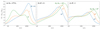 |
Fig. 1. Calculated effective radius ratio, ℛ, taking α = 0.1, Rin = 3RS and Rout = 5000RS. In panel (a), we show ℛ with a given value of M• but varying accretion rates. In panels (b) and (c), we fix |

3. Results
3.1. Vertical structure and emergent spectra
In this section, we present numerical results of vertical structure of the disk first, which can provide insights into the origin of the deviation between a self-consistent model and the blackbody disk model. Subsequently, we provide the SEDs and time lags predicted by the current model. We will compare these predictions with observational results and discuss the factors that influence them. Throughout this paper, we adopt RS = 2GM•/c2 as the Schwarzschild radius.
To numerically solve the above equations, we apply a finite difference method. We set two independent variables, ξ = log(τ0 − τ) and X = log(hν/mec2). We applied Nξ = 20 grids evenly spaced from ξmax = log τ0 to ξmin = −2 in the ξ space, and NX = 40 grids evenly spaced from Xmin = −8 to Xmax in the X space. To avoid cut-off errors, the determination of Xmax varies with R. The finite difference scheme for Kompaneets equation follows the same treatment as Chang & Cooper (1970). Since the above equations contain non-linear terms, we applied a Newton-Raphson method to solve the equations. To calculate the SED of the entire disk, we need to calculate the total Thomson scattering optical depth τ0(R) first. Once again, we applied the Newton-Raphson method to the equations of SS73 to solve for τ0(R). All the results presented in ST93 have been replicated in our study.
Here, we take an example of vertical structures at R = 5.16RS with log(M•/M⊙) = 8 and α = 0.1. By solving the equations outlined in Section 2.1, we obtain a self-consistent solution for the vertical structure of the accretion disk. Near the mid-plane of the disk, where  , electrons are in adequate contact with photons, we have
 (11)
(11)
where a is the radiation constant. The electron number density, Ne, can be obtained from derivative of Equation (2) with respect to τ, which gives
 (12)
(12)
with Prad = ∫dνϵν/3 being the radiation pressure. This indicates that Ne is determined by the second-order derivatives of gas and radiation pressure. It is obvious that the overall density falls towards the disk surface. Notably, when  , radiation pressure dominates over gas pressure at the mid-plane of the disk. Numerical calculation shows that the second-order derivative of radiation pressure is larger than that of gas pressure. With the second-order derivative of radiation pressure being constant at the mid-plane, Ne remains nearly constant towards the outer surface.
As the second-order derivative of gas pressure continuously increases and Te gradually deviates from Equation (11), Ne begins to decrease outward rapidly. In the present example, Ne decreases as Ne ∝ τ−2/3 while Te decreases as Te ∝ τ−1/4. With a rapid decrease of Ne, the free-free absorption becomes less significant outward and even becomes transparent for photons with hν/kBTe ≳ 7.85Te−7/4Ne1/2 (Czerny & Elvis 1987). Consequently, the radiation field begins to deviate from the blackbody spectrum at high frequency range. For photons with even higher frequencies, absorption is already transparent deep inside the disk at an optical depth τlast, where  , which is sufficient for photons to be Comptonized at such a high temperature. The outgoing spectrum above such frequency exhibits a Wein tail at around (2 ∼ 3)kBTe (Czerny & Elvis 1987; Ross et al. 1992).
Near the disk surface where τ0 − τ ≲ 1, as the density decreases, Compton cooling surpasses free-free cooling, and the temperature rises to balance disk heating; therefore, the temperature inversion shows up at the disk surface (see Figure 1 of ST93). Although temperature inversion occurs, photons cannot be thermalized to such high temperatures since the temperature inversion layer is optically thin for scattering. As a result, radiation at higher frequencies contains photons generated at deeper layers with higher temperatures, causing the emergent radiation from the disk surface peaks at higher frequencies than the blackbody spectrum, which results in that the emission at a specific wavelength emerges at larger radius in non-blackbody disks than in blackbody cases. In the present example with  , the canonical blackbody radiation at R = 5.16RS peaks at 721 Å while the present non-blackbody model yields a result of Reff, λ = 12.9Rs at the same wavelength, which is 2.5 times larger than the blackbody case.
We made an overall comparison of non-blackbody SEDs, with the blackbody cases under different M• and  , finding that the overall SEDs of non-blackbody disks also peak at higher frequencies and generally have a shallower slope than the blackbody cases. For a non-blackbody disk, changing
  can significantly affect the shape of the SED (see Figure A.1); with smaller
  , the SED slope becomes flatter at 103 ∼ 104 Å. The masses of the black holes have a clear influence on the intensity of flux, but have little influence on the overall shape of SEDs.
3.2. Effective radius
Figure 1 shows the dependence of ℛ on M• and  . It can be seen that the overall time lag teff, λ is approximately 1.2 − 2.6 times larger than in the blackbody case. Figure 1 (a) shows ℛ versus
  for a given M•. A single peak at longer wavelength bands is observed when the accretion rate is small with
  . As
. As  increases, the peak at longer wavelengths shifts towards shorter wavelengths and gradually diminishes while a peak at even shorter wavelengths gradually forms. Panels (b) and (c) in Figure 1 show predicted ℛ versus M• for given accretion rates of
  , respectively. It can be seen that M• affects ℛ weakly; instead, it changes the overall magnitude of ℛ and the position of its peaks. As M• increases, peaks of the ℛ shift to longer wavelengths with increases of their magnitudes. We fit Reff, λ at UV/optical wavelengths and found a relation via
  , yielding a relation of
  . It can be seen from the fitting that the ℛ is weakly correlated to M•, but more sensitive to
  .
.
The dependence of ℛ on M• and  can be explained according to the relative changes of the free-free absorption and electron scattering. As
  increases, the electron number density at inner region of the disk decreases as
  , while the electron temperature distribution at the mid-plane keeps unchanged according to SS73. Consequently, the σff is more likely to drop below the σT at inner regions, where the disk mainly radiates at higher frequencies. This leads the emergent spectrum to a greater deviation from blackbody spectrum at high frequencies. Therefore, ℛ gradually forms a peak at shorter wavelength range when increasing
  . According to SS73, we have transition radius in units of RS from the inner region to the outer region as
 (13)
(13)
where α0.1 = α/0.1 and M7 = M•/107 M⊙. Within the inner region, the electron temperature at mid-plane Tc decreases towards larger radii as Tc ∝ R−3/4, whereas Ne increases outwards as Ne ∝ R3/2. Consequently, the free-free absorption effect becomes more and more significant towards outer radii and therefore, with higher  , the ℛ drops towards smaller frequencies at ν ∼ 1016Hz. For a disk with smaller
  , a relatively smaller inner region is expected, which is inadequate for free-free absorption to increase to a sufficiently high level before it reaches the middle region of the disk; in this middel region, according to SS73, Ne decreases more rapidly outward than the Tc (with Ne ∝ R−33/20 and Tc ∝ R−9/10). This results in a decrease in σff toward the outer radius. Consequently, the ℛ increases towards longer wavelength continuously at relatively lower accretion rates.
To explain the behavior of ℛ with given  . We consider the rab and the overall temperature of the disk. The boundary of inner and middle regions rab is insensitive to M• (see Equation 13). Therefore, the M• cannot significantly affect the overall shape of ℛ. At shorter wavelengths, ℛ with smaller M• are generally larger than that of greater cases. This is because that a larger M• results in a relatively colder disk, where the absorption effects are more significant, as a result, the emergent spectrum from disks with higher M• deviates less from blackbody than that from disks with smaller M• at a certain frequency.
4. Comparison to observations
To make a suitable compareison of the current model with observations, we collected all the mapped AGNs listed in Table 1, along with their properties. Their M• values have been measured by the RM of broad emission lines, utilizing M• = fΔV2RBLR/G, where ΔV is the velocity width of the broad emission line, RBLR is the radius of the broad line region, and f is the virial factor or f-factor (see Du & Wang 2019 for more details). For simplicity, we take α = 0.1 for all cases described in this paper. We fixed the inner boundary at innermost stable circular orbit (ISCO) and the outer boundary at 5000RS. Since ℛ is found to be independent of inclinations and is primarily sensitive to  , we determined
  by fitting observations of ℛ − λ and Reff, λ − λ via minimization of χ2:
 (14)
(14)
where Robs, λi is the RM-measured radius at wavelength, λ, and σi is the error bar of  . Once
  is determined, we can estimate the inclination angle of disks by comparing the predicted SEDs with observational data. It is worthy to note that the above process offers a way to decouple the inclinations from accretion rates and black hole masses, which can be briefly summarized in three steps: (i) we first determine M• from RM of BLR; (ii) we then find the best-fit
  from ℛ − λ and teff, λ − λ relation, and (iii) we finally determine the inclination from SED fitting. During the ℛ − λ fittings, we excluded data from Swift/U and ground-based u-bands due to contamination by Balmer continuum emission. Solving the above equations for the entire accretion disk is time-consuming; therefore, we preset several
  values and find the ones with minimum χ2. The results are shown in Figure 2 and Appendix B. The left panels shown in figures display the effective radii, where the red lines represent time lags predicted by the current model, dashed lines represent the time lags in blackbody cases, and dots with error bars represent the observational data. The middle panels show results of ℛ, with red lines representing the predicted ℛ, and the error bars representing the observed ℛ. The right panels show the comparison of SEDs, where the red lines represent the SEDs predicted by the current model, dashed lines represent the SEDs of blackbody disk and the error bars or points show the observational data.
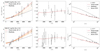 |
Fig. 2. Effective radii, effective radius ratios and SEDs for mapped AGNs. Left panels show Reff as a function of wavelength predicted by the current model for different preset accretion rates, in orange, while the red lines correspond to the best-fit |


It can be seen from the results that the predicted Reff, λ is able to aptly describe the observation in most cases. For most Seyfert 1 galaxies in our sample, a decreasing or a flattening tendency of ℛ has been seen at longer wavelengths, which is in good agreement with the model prediction. 50% of the targets have good SED fittings, for example, Fairall 9, Mrk 817, Mrk 110, NGC 4151, NGC 7469, and NGC 5548, with most of them above  . Also, 50% of the targets have a bad SED fit and most of them exhibit
  , for example, NGC 4593, Mrk 509, NGC 2617, MCG+08-11-011, and Ark 120. The bad SED fittings may be due to the non-simultaneous observation between SED and continuum RM, since it is not always feasible to fit the SED observed at one time epoch using the parameters obtained at another time epoch. Also, the M• values of these objects may be inaccurately estimated by applying the inaccurate f-factor, which will influence the Reff, λ and SED fitting. Moreover, the contamination of torus and host galaxies may contribute extra flux at longer wavelength and change the slope of SEDs, which will cause difficulty when fitting our predictions to the observational data points.
We also provide a comparison of the  fitted by the current model and previously obtained
  (see Table 2). The fitting results for Ark 120, MCG + 08-11-011, NGC 2617, Mrk 110. NGC 4593, Mrk 509 are in relatively good agreement with the results measured by Du & Wang (2019). While there are also 50% of the
  that are in good agreement with the measurement by other methods. The discrepancies may be due to different models applied when calculating
  . The previous research used the canonical blackbody model to measure the
  , whereas we chose to apply a non-blackbody one. Furthermore, the mismatch between observation epochs can also introduce discrepancies among the various measurement results. It should be noted that for Mrk 817, Kara et al. (2021) obtained the accretion rate by fitting effective radius τ, which is similar to the method presented here. Their result is in agreement with the
  fitted by the current model. We provide comments on fitting result for each source below.
Comparison of fitted  with other research studies.
Fairall 9: The current model outperforms the blackbody model in both RM data fitting and in SED fitting. The inclination angle estimated from SED fitting is relatively moderate for Seyfert 1 galaxies, but it is smaller than the result of  degree measured by Walton et al. (2013), this discrepancy may be attributed to the mismatch between epochs of RM campaign and SED observation.
Mrk 817: The RM data are well-fitted for time lags at λ > 2000 Å. The exclusion of U-band data affects the fitting only slightly. The current model fits the observational data better than the blackbody case in both RM data and SED. However, the inclination angle determined from the SED fitting is still relatively high compared to the result of < 40° obtained from Kara et al. (2021), possibly due to differences in the epochs of RM campaign and SED observation.
NGC 4593: The RM data are well-fitted for time lags with λ > 2000 Å and are better than the blackbody case for  . The observational data of ℛ exhibit a decreasing tendency at longer wavelengths, which is aptly predicted by the current model. However, the model predicted SED does not match the observational data, which may be due to host contamination or a mismatch between epochs of RM campaign and SED observation.
Mrk 110: The RM data are well-fitted and better than the blackbody case. The current model well predicts the decreasing tendency of ℛ at longer wavelengths. However, the model-predicted SED does not match the observational data. This discrepancy may be due to the underestimation of black hole mass or the super-Eddington nature of Mrk 110, which cannot be properly described by the current model. The mismatch of SED leaves the inclination undetermined. We note that the inclination measured by Walton et al. (2013) from Fe Kα is  degree.
NGC 4151: The current model shows significant improvement in fitting the RM lag and SED compared to the blackbody case. The inclination is comparatively large for the result of i < 20° determined by Keck et al. (2015) from the Fe Kα measurement; this is possibly due to host contamination or SED observation time mismatching the RM campaign epoch.
Mrk 509: The current model can fits the observation well, excluding U-band observational data. The predicted SED does not match the observational data, however, the slope favors the current model. This discrepancy may result from possible underestimation of the black hole mass or variability of the source. Determining the inclination requires better observational data and further studies of the model, the up-to-date measurement from the Fe Kα line by Walton et al. (2013) gave a result of < 18°.
NGC 7469: The RM data fit the current model well with λ > 1900 Å. Both the RM data and SED favor the current model over the blackbody one. The inclination determined from SED is in good agreement with result of < 54° measured by Walton et al. (2013).
NGC 2617: The current model is not a strong fit to the observations, but is still an improvement over the blackbody case. The changing-look nature of NGC 2617 makes fitting the time lag difficult. Due to the huge variability of NGC 2617, possible contamination of host galaxies, the SED is poorly fitted for λ > 4000 Å.
NGC 5548: Although the dimensionless accretion rate fitted is less than the criteria of  , both the RM data and SED are fitted very well. The present SED model is much better fit than the blackbody model. Its inclination is quite high compared to the results of 30° determined from Fe Kα line by Liu et al. (2010). A simultaneous SED observation with disk RM is necessary for a better fitting of inclination angle.
MCG +08-11-011: The current model is a better fit to the RM data than the blackbody case. The current model predicts a decreasing tendency of ℛ at longer wavelengths, which is in good agreement with observational data. The predicted SED by the current model does not match the observational data. However, it can be seen that the slope of it better follows the observational data than the blackbody case. The mismatch between SEDs is possibly due to the underestimated black hole mass or a mismatch in the epochs of the RM campaign and SED observation.
Ark 120: The quality of Disk-RM data are quite poor, but the data reveals some very unusual properties. It has been suggested that it contains a close binary of SMBHs (Li et al. 2019). If there are two accretion disks, the continuum reverberations will be complicated. A new campaign on this object is expected. Anyway, we provide inclination determined from Fe Kα measurement carried out by Walton et al. (2013) with a value of  degree.
Mrk 335: The current model is not a good fit to both the RM time lag and the SED. Mrk 335 is a super-Eddington AGN, with an accretion rate of  , which is beyond the descriptive capability of the current model. As discussed above, accretion disks with such a high accretion rate will become extremely slim; thus, they cannot be described by the thin disk model. Further studies are needed to determine the inclination; nevertheless, we suggest a reference result measured by Parker et al. (2014) of 65 ± 1 degree.
5. Conclusions and discussions
We applied a self-consistent model of the vertical structures of the Shakura-Sunyev disk (Shimura & Takahara 1993) to explain the sizes measured by disk reverberation mapping. The model considers the effects of electron scattering, resulting in a non-blackbody radiation profile with the peak shifting to higher frequencies than blackbody cases. We have drawn the following conclusions
-
The wavelength-dependent time lags, teff, λ, effective radius ratio, ℛ, and, finally, the SEDs of non-blackbody disks are predicted by the current model.
-
The well-known tension between the mapped radii and the blackbody radii can be self-consistently alleviated by the effects of radiation transfer along the vertical structure of accretion disks. The mapped radii, which are a few times of the blackbody approximation, are consistent with the present predictions.
-
It is found that teff, λ and ℛ are sensitive to
 and less so to M•, allowing us to determine
  from Reff, λ after BLR RM for M•. This completely disentangles the degeneracy of inclinations of accretion disks from
  when fitting the continuum.We can use the mapped radii to obtain the inclinations, SMBH masses and accretion rates of AGN central engines independently.
 -
Generally, disk effective radii, Reff, λ, can be fitted quite well but a few AGNs are poorly explained for the given M•. We find that 50% of the targets are good SED fits and the discrepancies may be due to contamination of host or torus and the non-simultaneous data collection of SEDs with the continuum RM. The inaccurate estimations of the f factor and SMBH masses may affect the whole fitting process.
To improve the fit of the accretion rate and inclination angle of an accretion disk, the estimation of black hole mass needs to be improved. A better way is the dynamical modeling of RM of broad Hβ line, which will provide much more reliable M• result (Pancoast et al. 2011; Li et al. 2018); in particular, M• can be measured with higher accuracy by the analysis SpectroAstrometry and RM (SARM, see Wang et al. 2020; GRAVITY Collaboration 2021, for the first and second applications to 3C 273 and NGC 3783, respectively). In addition, the SED should be obtained simultaneously with the continuum RM observation.
In the current model, we have not included the hot corona and its irradiation effects. In the lamp-post model, the hot corona above the central black hole irradiates the entire disk in X-ray, which can affect the vertical structures of accretion disks in surface temperature distribution, enhance the ionization of hydrogen atoms, finally, it may affect density distributions in vertical direction. We did not take general relativity effects into our consideration either, which have a clear influence on the disk structure and can influence time lags of radiation. The above effect will be modeled and discussed in the future work.
Additionally, we did not account for radiation transfer in radial direction and heavy element abundance. As mentioned in the basic assumption, we did not consider the detailed ionization of disks or bound-free and bound-bound absorption effects. The opacity of gas at the disk surface will be contributed mainly by bound-bound absorption and bound-free absorption for accretion disks with high masses and low accretion rates, where the temperature is relatively low. This effect can cause discrepancy between the current model prediction and observation if  . The detailed ionization, bound-bound, and bound-free absorption details will be taken into consideration in the forthcoming paper.
Moreover, the current model only applies to sub-Eddington moderately super-Eddington accretion disks. It is known that some AGNs are undergoing super-Eddington accretion (Du et al. 2014); for instance, the mapped Mrk 335 and Mrk 421 ( found in Li et al. 2018) have super-Eddington accretion rates (Hu et al. 2015; Cackett et al. 2018), namely, they are so high that the code meant to solve the vertical structure functions does not converge. In the context of super-Eddington accretion, the vertical structure of slim disks (Abramowicz et al. 1988; Wang & Zhou 1999) should be calculated (Wang et al. 1999; Shimura & Manmoto 2003) for super-Eddington AGNs in a future paper.
Neglecting the geometric thickness of the disk and general relativistic effects of photon propagation, this effective radius is fully independent of inclinations of the disks. If the corona as a lamp-post is included, inclination effects should be considered in a future paper.
We take cosmological constants H0 = 70 km s−1 Mpc−1, ΩM = 0.27 and ΩΛ = 0.73 in this paper.
Acknowledgments
Drs. M.-Y. Sun, Y.-R. Li and P. Du are acknowledged for helpful discussions. J.-M.W. thanks the support by the National Key R&D Program of China through grants 2016YFA0400701 and 2020YFC2201400 by NSFC-11991050, -11991054 and -12333003. This work makes use of NUMPY (Harris et al. 2020), SCIPY (Virtanen et al. 2020), astropy (Astropy Collaboration 2022) and MATPLOTLIB (Hunter 2007).
References
- Abramowicz, M. A., Czerny, B., Lasota, J. P., & Szuszkiewicz, E. 1988, ApJ, 332, 646 [Google Scholar]
- Astropy Collaboration (Price-Whelan, A. M., et al.) 2022, ApJ, 935, 167 [NASA ADS] [CrossRef] [Google Scholar]
- Brown, M. J. I., Duncan, K. J., Landt, H., et al. 2019, MNRAS, 489, 3351 [Google Scholar]
- Cackett, E. M., Horne, K., & Winkler, H. 2007, MNRAS, 380, 669 [Google Scholar]
- Cackett, E. M., Chiang, C.-Y., McHardy, I., et al. 2018, ApJ, 857, 53 [NASA ADS] [CrossRef] [Google Scholar]
- Chang, J. S., & Cooper, G. 1970, J. Comput. Phys., 6, 1 [Google Scholar]
- Czerny, B., & Elvis, M. 1987, ApJ, 321, 305 [NASA ADS] [CrossRef] [Google Scholar]
- Du, P., & Wang, J.-M. 2019, ApJ, 886, 42 [NASA ADS] [CrossRef] [Google Scholar]
- Du, P., Hu, C., Lu, K.-X., et al. 2014, ApJ, 782, 45 [NASA ADS] [CrossRef] [Google Scholar]
- Edelson, R., Gelbord, J. M., Horne, K., et al. 2015, ApJ, 806, 129 [NASA ADS] [CrossRef] [Google Scholar]
- Edelson, R., Gelbord, J., Cackett, E., et al. 2017, ApJ, 840, 41 [NASA ADS] [CrossRef] [Google Scholar]
- Edelson, R., Gelbord, J., Cackett, E., et al. 2019, ApJ, 870, 123 [NASA ADS] [CrossRef] [Google Scholar]
- Fausnaugh, M. M., Denney, K. D., Barth, A. J., et al. 2016, ApJ, 821, 56 [Google Scholar]
- Fausnaugh, M. M., Starkey, D. A., Horne, K., et al. 2018, ApJ, 854, 107 [NASA ADS] [CrossRef] [Google Scholar]
- Fian, C., Chelouche, D., Kaspi, S., et al. 2023, A&A, 672, A132 [NASA ADS] [CrossRef] [EDP Sciences] [Google Scholar]
- Graham, M. J., Kulkarni, S. R., Bellm, E. C., et al. 2019, PASP, 131, 078001 [Google Scholar]
- GRAVITY Collaboration (Amorim, A., et al.) 2021, A&A, 654, A85 [NASA ADS] [CrossRef] [EDP Sciences] [Google Scholar]
- Grupe, D., Komossa, S., Leighly, K. M., & Page, K. L. 2010, ApJS, 187, 64 [NASA ADS] [CrossRef] [Google Scholar]
- Guilbert, P. W., & Stepney, S. 1985, MNRAS, 212, 523 [NASA ADS] [CrossRef] [Google Scholar]
- Hall, P. B., Sarrouh, G. T., & Horne, K. 2018, ApJ, 854, 93 [Google Scholar]
- Harris, C. R., Millman, K. J., van der Walt, S. J., et al. 2020, Nature, 585, 357 [NASA ADS] [CrossRef] [Google Scholar]
- Hernández Santisteban, J. V., Edelson, R., Horne, K., et al. 2020, MNRAS, 498, 5399 [CrossRef] [Google Scholar]
- Hu, C., Du, P., Lu, K.-X., et al. 2015, ApJ, 804, 138 [Google Scholar]
- Hunter, J. D. 2007, Comput. Sci. Eng., 9, 90 [NASA ADS] [CrossRef] [Google Scholar]
- Kaastra, J. S., Petrucci, P. O., Cappi, M., et al. 2011, A&A, 534, A36 [NASA ADS] [CrossRef] [EDP Sciences] [Google Scholar]
- Kammoun, E. S., Domček, V., Svoboda, J., Dovčiak, M., & Matt, G. 2019, MNRAS, 485, 239 [NASA ADS] [CrossRef] [Google Scholar]
- Kammoun, E. S., Robin, L., Papadakis, I. E., Dovčiak, M., & Panagiotou, C. 2023, MNRAS, 526, 138 [NASA ADS] [CrossRef] [Google Scholar]
- Kara, E., Mehdipour, M., Kriss, G. A., et al. 2021, ApJ, 922, 151 [NASA ADS] [CrossRef] [Google Scholar]
- Kara, E., Barth, A. J., Cackett, E. M., et al. 2023, ApJ, 947, 62 [NASA ADS] [CrossRef] [Google Scholar]
- Keck, M. L., Brenneman, L. W., Ballantyne, D. R., et al. 2015, ApJ, 806, 149 [NASA ADS] [CrossRef] [Google Scholar]
- Kompaneets, A. S. 1957, Sov. J. Exp. Theor. Phys., 4, 730 [Google Scholar]
- Laor, A., & Netzer, H. 1989, MNRAS, 238, 897 [NASA ADS] [CrossRef] [Google Scholar]
- Li, Y.-R., Songsheng, Y.-Y., Qiu, J., et al. 2018, ApJ, 869, 137 [CrossRef] [Google Scholar]
- Li, Y.-R., Wang, J.-M., Zhang, Z.-X., et al. 2019, ApJS, 241, 33 [Google Scholar]
- Liu, Y., Elvis, M., McHardy, I. M., et al. 2010, ApJ, 710, 1228 [NASA ADS] [CrossRef] [Google Scholar]
- Lobban, A. P., Zola, S., Pajdosz-Śmierciak, U., et al. 2020, MNRAS, 494, 1165 [NASA ADS] [CrossRef] [Google Scholar]
- McHardy, I. M., Connolly, S. D., Horne, K., et al. 2018, MNRAS, 480, 2881 [NASA ADS] [CrossRef] [Google Scholar]
- Meyer-Hofmeister, E., & Meyer, F. 2011, A&A, 527, A127 [NASA ADS] [CrossRef] [EDP Sciences] [Google Scholar]
- Pahari, M., McHardy, I. M., Vincentelli, F., et al. 2020, MNRAS, 494, 4057 [NASA ADS] [CrossRef] [Google Scholar]
- Pal, M., Dewangan, G. C., Connolly, S. D., & Misra, R. 2017, MNRAS, 466, 1777 [NASA ADS] [CrossRef] [Google Scholar]
- Pancoast, A., Brewer, B. J., & Treu, T. 2011, ApJ, 730, 139 [NASA ADS] [CrossRef] [Google Scholar]
- Parker, M. L., Wilkins, D. R., Fabian, A. C., et al. 2014, MNRAS, 443, 1723 [NASA ADS] [CrossRef] [Google Scholar]
- Porquet, D., Reeves, J. N., Matt, G., et al. 2018, A&A, 609, A42 [NASA ADS] [CrossRef] [EDP Sciences] [Google Scholar]
- Rees, M. J. 1984, ARA&A, 22, 471 [Google Scholar]
- Ross, R. R., Fabian, A. C., & Mineshige, S. 1992, MNRAS, 258, 189 [NASA ADS] [CrossRef] [Google Scholar]
- Salvesen, G. 2022, ApJ, 940, L22 [NASA ADS] [CrossRef] [Google Scholar]
- Shakura, N. I., & Sunyaev, R. A. 1973, A&A, 24, 337 [NASA ADS] [Google Scholar]
- Shappee, B. J., Prieto, J. L., Grupe, D., et al. 2014, ApJ, 788, 48 [Google Scholar]
- Shimura, T., & Manmoto, T. 2003, MNRAS, 338, 1013 [NASA ADS] [CrossRef] [Google Scholar]
- Shimura, T., & Takahara, F. 1993, ApJ, 419, 78 [NASA ADS] [CrossRef] [Google Scholar]
- Shimura, T., & Takahara, F. 1995, ApJ, 440, 610 [NASA ADS] [CrossRef] [Google Scholar]
- Tripathi, S., McGrath, K. M., Gallo, L. C., et al. 2020, MNRAS, 499, 1266 [NASA ADS] [CrossRef] [Google Scholar]
- Vincentelli, F. M., McHardy, I., Cackett, E. M., et al. 2021, MNRAS, 504, 4337 [CrossRef] [Google Scholar]
- Virtanen, P., Gommers, R., Oliphant, T. E., et al. 2020, Nat. Methods, 17, 261 [Google Scholar]
- Walton, D. J., Nardini, E., Fabian, A. C., Gallo, L. C., & Reis, R. C. 2013, MNRAS, 428, 2901 [NASA ADS] [CrossRef] [Google Scholar]
- Wang, J.-M., & Zhou, Y.-Y. 1999, ApJ, 516, 420 [NASA ADS] [CrossRef] [Google Scholar]
- Wang, J.-M., Szuszkiewicz, E., Lu, F.-J., & Zhou, Y.-Y. 1999, ApJ, 522, 839 [NASA ADS] [CrossRef] [Google Scholar]
- Wang, J.-M., Songsheng, Y.-Y., Li, Y.-R., Du, P., & Zhang, Z.-X. 2020, Nat. Astron., 4, 517 [NASA ADS] [CrossRef] [Google Scholar]
Appendix A: SED predicted by the present model
For reader’s convenience, we show how the SED changes with  . For more details, see Shimura & Takahara (1995).
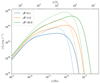 |
Fig. A.1. SEDs of accretion disks with M• = 108 M⊙. The solid lines are the SEDs predicted by the present model while the dashed lines are the SEDs for canonical blackbody models. The blue, orange, green lines represent the accretion disks with accretion rates of |
Appendix B: Fitting result of the present model
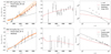 |
Fig. B.1. Effective radii, effective radius ratios and SEDs for mapped AGNs. Left panels show Reff as a function of wavelength predicted by the current model for different preset accretion rates, in orange, while the red lines correspond to the best-fit |


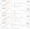 |
Fig. B.1. continued. |
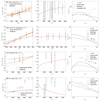 |
Fig. B.1. continued. Akn 120 and Mrk 335 are most poorly explained, see text for details. |
All Tables
All Figures
|
Fig. 1. Calculated effective radius ratio, ℛ, taking α = 0.1, Rin = 3RS and Rout = 5000RS. In panel (a), we show ℛ with a given value of M• but varying accretion rates. In panels (b) and (c), we fix |
| In the text | |
|
Fig. 2. Effective radii, effective radius ratios and SEDs for mapped AGNs. Left panels show Reff as a function of wavelength predicted by the current model for different preset accretion rates, in orange, while the red lines correspond to the best-fit |
| In the text | |
|
Fig. A.1. SEDs of accretion disks with M• = 108 M⊙. The solid lines are the SEDs predicted by the present model while the dashed lines are the SEDs for canonical blackbody models. The blue, orange, green lines represent the accretion disks with accretion rates of |
| In the text | |
|
Fig. B.1. Effective radii, effective radius ratios and SEDs for mapped AGNs. Left panels show Reff as a function of wavelength predicted by the current model for different preset accretion rates, in orange, while the red lines correspond to the best-fit |
| In the text | |
|
Fig. B.1. continued. |
| In the text | |
|
Fig. B.1. continued. Akn 120 and Mrk 335 are most poorly explained, see text for details. |
| In the text | |
Current usage metrics show cumulative count of Article Views (full-text article views including HTML views, PDF and ePub downloads, according to the available data) and Abstracts Views on Vision4Press platform.
Data correspond to usage on the plateform after 2015. The current usage metrics is available 48-96 hours after online publication and is updated daily on week days.
Initial download of the metrics may take a while.