| Issue |
A&A
Volume 695, March 2025
|
|
|---|---|---|
| Article Number | A282 | |
| Number of page(s) | 24 | |
| Section | Cosmology (including clusters of galaxies) | |
| DOI | https://doi.org/10.1051/0004-6361/202451347 | |
| Published online | 03 April 2025 | |
Euclid preparation
LXVI. Impact of line-of-sight projections on the covariance between galaxy cluster multi-wavelength observable properties: insights from hydrodynamic simulations
1
INAF-Osservatorio di Astrofisica e Scienza dello Spazio di Bologna, Via Piero Gobetti 93/3, 40129 Bologna, Italy
2
IFPU, Institute for Fundamental Physics of the Universe, Via Beirut 2, 34151 Trieste, Italy
3
Dipartimento di Fisica e Astronomia “Augusto Righi” – Alma Mater Studiorum Università di Bologna, Via Piero Gobetti 93/2, 40129 Bologna, Italy
4
ICSC – Centro Nazionale di Ricerca in High Performance Computing, Big Data e Quantum Computing, Via Magnanelli 2, Bologna, Italy
5
Dipartimento di Fisica – Sezione di Astronomia, Università di Trieste, Via Tiepolo 11, 34131 Trieste, Italy
6
INAF-Osservatorio Astronomico di Trieste, Via G. B. Tiepolo 11, 34143 Trieste, Italy
7
INFN, Sezione di Trieste, Via Valerio 2, 34127 Trieste, TS, Italy
8
INAF-Osservatorio Astronomico di Brera, Via Brera 28, 20122 Milano, Italy
9
Universitäts-Sternwarte München, Fakultät für Physik, Ludwig-Maximilians-Universität München, Scheinerstrasse 1, 81679 München, Germany
10
INFN-Bologna, Via Irnerio 46, 40126 Bologna, Italy
11
Istituto Nazionale di Fisica Nucleare, Sezione di Bologna, Via Irnerio 46, 40126 Bologna, Italy
12
Laboratoire Univers et Théorie, Observatoire de Paris, Université PSL, Université Paris Cité, CNRS, 92190 Meudon, France
13
Institut d’Astrophysique de Paris, 98 bis Boulevard Arago, 75014 Paris, France
14
Institut d’Astrophysique de Paris, UMR 7095, CNRS, and Sorbonne Université, 98 bis boulevard Arago, 75014 Paris, France
15
School of Physics, HH Wills Physics Laboratory, University of Bristol, Tyndall Avenue, Bristol BS8 1TL, UK
16
INFN-Sezione di Bologna, Viale Berti Pichat 6/2, 40127 Bologna, Italy
17
Universität Bonn, Argelander-Institut für Astronomie, Auf dem Hügel 71, 53121 Bonn, Germany
18
Université Paris-Saclay, Université Paris Cité, CEA, CNRS, AIM, 91191 Gif-sur-Yvette, France
19
Dipartimento di Fisica, Sapienza Università di Roma, Piazzale Aldo Moro 2, 00185 Roma, Italy
20
Department of Astronomy, University of Geneva, Ch. d’Ecogia 16, 1290 Versoix, Switzerland
21
Univ. Grenoble Alpes, CNRS, Grenoble INP, LPSC-IN2P3, 53, Avenue des Martyrs, 38000 Grenoble, France
22
Institut für Theoretische Physik, University of Heidelberg, Philosophenweg 16, 69120 Heidelberg, Germany
23
Zentrum für Astronomie, Universität Heidelberg, Philosophenweg 12, 69120 Heidelberg, Germany
24
School of Mathematics and Physics, University of Surrey, Guildford, Surrey GU2 7XH, UK
25
SISSA, International School for Advanced Studies, Via Bonomea 265, 34136 Trieste, TS, Italy
26
Dipartimento di Fisica e Astronomia, Università di Bologna, Via Gobetti 93/2, 40129 Bologna, Italy
27
INAF-Osservatorio Astrofisico di Torino, Via Osservatorio 20, 10025 Pino Torinese, (TO), Italy
28
Dipartimento di Fisica, Università di Genova, Via Dodecaneso 33, 16146 Genova, Italy
29
INFN-Sezione di Genova, Via Dodecaneso 33, 16146 Genova, Italy
30
Department of Physics “E. Pancini”, University Federico II, Via Cinthia 6, 80126 Napoli, Italy
31
INAF-Osservatorio Astronomico di Capodimonte, Via Moiariello 16, 80131 Napoli, Italy
32
INFN section of Naples, Via Cinthia 6, 80126 Napoli, Italy
33
Instituto de Astrofísica e Ciências do Espaço, Universidade do Porto, CAUP, Rua das Estrelas, PT4150-762 Porto, Portugal
34
Dipartimento di Fisica, Università degli Studi di Torino, Via P. Giuria 1, 10125 Torino, Italy
35
INFN-Sezione di Torino, Via P. Giuria 1, 10125 Torino, Italy
36
INAF-IASF Milano, Via Alfonso Corti 12, 20133 Milano, Italy
37
Centro de Investigaciones Energéticas, Medioambientales y Tecnológicas (CIEMAT), Avenida Complutense 40, 28040 Madrid, Spain
38
Port d’Informació Científica, Campus UAB, C. Albareda s/n, 08193 Bellaterra, (Barcelona), Spain
39
Institute for Theoretical Particle Physics and Cosmology (TTK), RWTH Aachen University, 52056 Aachen, Germany
40
INAF-Osservatorio Astronomico di Roma, Via Frascati 33, 00078 Monteporzio Catone, Italy
41
Dipartimento di Fisica e Astronomia “Augusto Righi” – Alma Mater Studiorum Università di Bologna, Viale Berti Pichat 6/2, 40127 Bologna, Italy
42
Instituto de Astrofísica de Canarias, Calle Vía Láctea s/n, 38204 San Cristóbal de La Laguna, Tenerife, Spain
43
Institute for Astronomy, University of Edinburgh, Royal Observatory, Blackford Hill, Edinburgh EH9 3HJ, UK
44
Jodrell Bank Centre for Astrophysics, Department of Physics and Astronomy, University of Manchester, Oxford Road, Manchester M13 9PL, UK
45
European Space Agency/ESRIN, Largo Galileo Galilei 1, 00044 Frascati, Roma, Italy
46
ESAC/ESA, Camino Bajo del Castillo, s/n, Urb. Villafranca del Castillo, 28692 Villanueva de la Cañada, Madrid, Spain
47
Université Claude Bernard Lyon 1, CNRS/IN2P3, IP2I Lyon, UMR 5822, Villeurbanne F-69100, France
48
Institute of Physics, Laboratory of Astrophysics, Ecole Polytechnique Fédérale de Lausanne (EPFL), Observatoire de Sauverny, 1290 Versoix, Switzerland
49
UCB Lyon 1, CNRS/IN2P3, IUF, IP2I Lyon, 4 Rue Enrico Fermi, 69622 Villeurbanne, France
50
Departamento de Física, Faculdade de Ciências, Universidade de Lisboa, Edifício C8, Campo Grande, PT1749-016 Lisboa, Portugal
51
Instituto de Astrofísica e Ciências do Espaço, Faculdade de Ciências, Universidade de Lisboa, Campo Grande, 1749-016 Lisboa, Portugal
52
INAF-Istituto di Astrofisica e Planetologia Spaziali, Via del Fosso del Cavaliere, 100, 00100 Roma, Italy
53
INAF-Osservatorio Astronomico di Padova, Via dell’Osservatorio 5, 35122 Padova, Italy
54
Max Planck Institute for Extraterrestrial Physics, Giessenbachstr. 1, 85748 Garching, Germany
55
Institute of Theoretical Astrophysics, University of Oslo, PO Box 1029 Blindern, 0315 Oslo, Norway
56
Jet Propulsion Laboratory, California Institute of Technology, 4800 Oak Grove Drive, Pasadena, CA 91109, USA
57
Department of Physics, Lancaster University, Lancaster LA1 4YB, UK
58
Felix Hormuth Engineering, Goethestr. 17, 69181 Leimen, Germany
59
Technical University of Denmark, Elektrovej 327, 2800 Kgs. Lyngby, Denmark
60
Cosmic Dawn Center (DAWN), Denmark
61
Max-Planck-Institut für Astronomie, Königstuhl 17, 69117 Heidelberg, Germany
62
Department of Physics and Helsinki Institute of Physics, Gustaf Hällströmin katu 2, 00014 University of Helsinki, Finland
63
Aix-Marseille Université, CNRS/IN2P3, CPPM, Marseille, France
64
Université de Genève, Département de Physique Théorique and Centre for Astroparticle Physics, 24 Quai Ernest-Ansermet, CH-1211 Genève 4, Switzerland
65
Department of Physics, PO Box 64 00014 University of Helsinki, Finland
66
Helsinki Institute of Physics, Gustaf Hällströmin katu 2, University of Helsinki, Helsinki, Finland
67
NOVA Optical Infrared Instrumentation Group at ASTRON, Oude Hoogeveensedijk 4, 7991 PD Dwingeloo, The Netherlands
68
Dipartimento di Fisica “Aldo Pontremoli”, Università degli Studi di Milano, Via Celoria 16, 20133 Milano, Italy
69
INFN-Sezione di Milano, Via Celoria 16, 20133 Milano, Italy
70
INFN-Sezione di Roma, Piazzale Aldo Moro, 2 – c/o Dipartimento di Fisica, Edificio G. Marconi, 00185 Roma, Italy
71
Aix-Marseille Université, CNRS, CNES, LAM, Marseille, France
72
Department of Physics, Institute for Computational Cosmology, Durham University, South Road, Durham DH1 3LE, UK
73
Université Côte d’Azur, Observatoire de la Côte d’Azur, CNRS, Laboratoire Lagrange, Bd de l’Observatoire, CS 34229, 06304 Nice Cedex 4, France
74
Université Paris Cité, CNRS, Astroparticule et Cosmologie, 75013 Paris, France
75
Institut de Física d’Altes Energies (IFAE), The Barcelona Institute of Science and Technology, Campus UAB, 08193 Bellaterra, (Barcelona), Spain
76
European Space Agency/ESTEC, Keplerlaan 1, 2201 AZ Noordwijk, The Netherlands
77
School of Mathematics, Statistics and Physics, Newcastle University, Herschel Building, Newcastle-upon-Tyne NE1 7RU, UK
78
Department of Physics and Astronomy, University of Aarhus, Ny Munkegade 120, DK-8000 Aarhus C, Denmark
79
Space Science Data Center, Italian Space Agency, Via del Politecnico snc, 00133 Roma, Italy
80
Centre National d’Etudes Spatiales – Centre spatial de Toulouse, 18 Avenue Edouard Belin, 31401 Toulouse Cedex 9, France
81
Institute of Space Science, Str. Atomistilor, Nr. 409 Măgurele, Ilfov 077125, Romania
82
Dipartimento di Fisica e Astronomia “G. Galilei”, Università di Padova, Via Marzolo 8, 35131 Padova, Italy
83
INFN-Padova, Via Marzolo 8, 35131 Padova, Italy
84
Institut de Recherche en Astrophysique et Planétologie (IRAP), Université de Toulouse, CNRS, UPS, CNES, 14 Av. Edouard Belin, 31400 Toulouse, France
85
Université St Joseph; Faculty of Sciences, Beirut, Lebanon
86
Departamento de Física, FCFM, Universidad de Chile, Blanco Encalada 2008, Santiago, Chile
87
Universität Innsbruck, Institut für Astro- und Teilchenphysik, Technikerstr. 25/8, 6020 Innsbruck, Austria
88
Institut d’Estudis Espacials de Catalunya (IEEC), Edifici RDIT, Campus UPC, 08860 Castelldefels, Barcelona, Spain
89
Institute of Space Sciences (ICE, CSIC), Campus UAB, Carrer de Can Magrans, s/n, 08193 Barcelona, Spain
90
Satlantis, University Science Park, Sede Bld 48940, Leioa-Bilbao, Spain
91
Instituto de Astrofísica e Ciências do Espaço, Faculdade de Ciências, Universidade de Lisboa, Tapada da Ajuda, 1349-018 Lisboa, Portugal
92
Universidad Politécnica de Cartagena, Departamento de Electrónica y Tecnología de Computadoras, Plaza del Hospital 1, 30202 Cartagena, Spain
93
Kapteyn Astronomical Institute, University of Groningen, PO Box 800 9700 AV Groningen, The Netherlands
94
Infrared Processing and Analysis Center, California Institute of Technology, Pasadena, CA 91125, USA
95
INAF, Istituto di Radioastronomia, Via Piero Gobetti 101, 40129 Bologna, Italy
96
Astronomical Observatory of the Autonomous Region of the Aosta Valley (OAVdA), Loc. Lignan 39, I-11020 Nus, (Aosta Valley), Italy
97
ICL, Junia, Université Catholique de Lille, LITL, 59000 Lille, France
98
Instituto de Física Teórica UAM-CSIC, Campus de Cantoblanco, 28049 Madrid, Spain
99
CERCA/ISO, Department of Physics, Case Western Reserve University, 10900 Euclid Avenue, Cleveland, OH 44106, USA
100
Dipartimento di Fisica e Scienze della Terra, Università degli Studi di Ferrara, Via Giuseppe Saragat 1, 44122 Ferrara, Italy
101
Istituto Nazionale di Fisica Nucleare, Sezione di Ferrara, Via Giuseppe Saragat 1, 44122 Ferrara, Italy
102
Kavli Institute for the Physics and Mathematics of the Universe (WPI), University of Tokyo, Kashiwa, Chiba 277-8583, Japan
103
Minnesota Institute for Astrophysics, University of Minnesota, 116 Church St SE, Minneapolis, MN 55455, USA
104
Institute Lorentz, Leiden University, Niels Bohrweg 2, 2333 CA, Leiden, The Netherlands
105
Institute for Astronomy, University of Hawaii, 2680 Woodlawn Drive, Honolulu, HI 96822, USA
106
Department of Physics & Astronomy, University of California Irvine, Irvine, CA 92697, USA
107
Department of Astronomy & Physics and Institute for Computational Astrophysics, Saint Mary’s University, 923 Robie Street, Halifax, Nova Scotia B3H 3C3, Canada
108
Departamento Física Aplicada, Universidad Politécnica de Cartagena, Campus Muralla del Mar, 30202 Cartagena, Murcia, Spain
109
Université Paris-Saclay, CNRS, Institut d’Astrophysique Spatiale, 91405 Orsay, France
110
Department of Physics, Oxford University, Keble Road, Oxford OX1 3RH, UK
111
Institute of Cosmology and Gravitation, University of Portsmouth, Portsmouth PO1 3FX, UK
112
Department of Computer Science, Aalto University, PO Box 15400 Espoo FI-00 076, Finland
113
Ruhr University Bochum, Faculty of Physics and Astronomy, Astronomical Institute (AIRUB), German Centre for Cosmological Lensing (GCCL), 44780 Bochum, Germany
114
DARK, Niels Bohr Institute, University of Copenhagen, Jagtvej 155, 2200 Copenhagen, Denmark
115
Department of Physics and Astronomy, Vesilinnantie 5, 20014 University of Turku, Finland
116
Serco for European Space Agency (ESA), Camino Bajo del Castillo s/n, Urbanizacion Villafranca del Castillo, Villanueva de la Cañada, 28692 Madrid, Spain
117
ARC Centre of Excellence for Dark Matter Particle Physics, Melbourne, Australia
118
Centre for Astrophysics & Supercomputing, Swinburne University of Technology, Hawthorn, Victoria 3122, Australia
119
School of Physics and Astronomy, Queen Mary University of London, Mile End Road, London E1 4NS, UK
120
Department of Physics and Astronomy, University of the Western Cape, Bellville, Cape Town 7535, South Africa
121
ICTP South American Institute for Fundamental Research, Instituto de Física Teórica, Universidade Estadual Paulista, São Paulo, Brazil
122
Oskar Klein Centre for Cosmoparticle Physics, Department of Physics, Stockholm University, Stockholm SE-106 91, Sweden
123
Astrophysics Group, Blackett Laboratory, Imperial College London, London SW7 2AZ, UK
124
INAF-Osservatorio Astrofisico di Arcetri, Largo E. Fermi 5, 50125 Firenze, Italy
125
Centro de Astrofísica da Universidade do Porto, Rua das Estrelas, 4150-762 Porto, Portugal
126
Institute of Astronomy, University of Cambridge, Madingley Road, Cambridge CB3 0HA, UK
127
Department of Astrophysics, University of Zurich, Winterthurerstrasse 190, 8057 Zurich, Switzerland
128
Dipartimento di Fisica, Università degli studi di Genova, and INFN-Sezione di Genova, Via Dodecaneso 33, 16146 Genova, Italy
129
Theoretical astrophysics, Department of Physics and Astronomy, Uppsala University, Box 515, 751 20 Uppsala, Sweden
130
Department of Physics, Royal Holloway, University of London, London TW20 0EX, UK
131
Mullard Space Science Laboratory, University College London, Holmbury St Mary, Dorking, Surrey RH5 6NT, UK
132
Department of Astrophysical Sciences, Peyton Hall, Princeton University, Princeton, NJ 08544, USA
133
Cosmic Dawn Center (DAWN)
134
Niels Bohr Institute, University of Copenhagen, Jagtvej 128, 2200 Copenhagen, Denmark
135
Center for Cosmology and Particle Physics, Department of Physics, New York University, New York, NY 10003, USA
136
Center for Computational Astrophysics, Flatiron Institute, 162 5th Avenue, 10010 New York, NY, USA
⋆ Corresponding author; antonio.ragagnin@unibo.it
Received:
2
July
2024
Accepted:
5
December
2024
Context. Cluster cosmology can benefit from combining multi-wavelength studies. In turn, these studies benefit from a characterisation of the correlation coefficients among different mass-observable relations.
Aims. In this work, we aim to provide information on the scatter, skewness, and covariance of various mass-observable relations in galaxy clusters in cosmological hydrodynamic simulations. This information will help future analyses improve the general approach to accretion histories and projection effects, as well as to model mass-observable relations for cosmology studies.
Methods. We identified galaxy clusters in Magneticum Box2b simulations with masses of M200c > 1014 M⊙ at redshifts of z = 0.24 and z = 0.90. Our analysis included Euclid-derived properties such as richness, stellar mass, lensing mass, and concentration. Additionally, we investigated complementary multi-wavelength data, including X-ray luminosity, integrated Compton-y parameter, gas mass, and temperature. We then examined the impact of projection effects on mass-observable residuals and correlations.
Results. We find that at intermediate redshift (z = 0.24), projection effects have the greatest impact of lensing concentration, richness, and gas mass in terms of the scatter and skewness of the log-residuals of scaling relations. The contribution of projection effects can be significant enough to boost a spurious hot- versus cold-baryon correlations and consequently hide underlying correlations due to halo accretion histories. At high redshift (z = 0.9), the richness has a much lower scatter (of log-residuals), while the quantity that is most impacted by projection effects is the lensing mass. The lensing concentration reconstruction, in particular, is affected by deviations of the reduced-shear profile shape from that derived using a Navarro-Frenk-White (NFW) profile; the amount of interlopers in the line of sight, on the other hand, is not as important.
Key words: methods: numerical / methods: statistical / galaxies: clusters: general / galaxies: clusters: intracluster medium / galaxies: halos
© The Authors 2025
 Open Access article, published by EDP Sciences, under the terms of the Creative Commons Attribution License (https://creativecommons.org/licenses/by/4.0), which permits unrestricted use, distribution, and reproduction in any medium, provided the original work is properly cited.
This article is published in open access under the Subscribe to Open model. Subscribe to A&A to support open access publication.
1. Introduction
Galaxy clusters are the largest gravitationally bound, collapsed, and virialised structures in our Universe. They represent unique laboratories for testing cosmological models, galaxy evolution, and thermodynamics of the intracluster medium (ICM, see Kravtsov & Borgani 2012, for a review on galaxy clusters). With respect galaxy cluster cosmology studies (see e.g. Rozo et al. 2010; Bocquet et al. 2019), an accurate characterisation of the selection function and of the mass-observable scaling relations requires a consideration of the dominant systematic uncertainties (see the review on the cluster mass scale in Pratt et al. 2019).
Cluster masses cannot be observed directly and their reconstruction requires both a number of assumptions and high-quality data (see e.g. Meneghetti et al. 2010). This means that precise estimates are rare (Okabe et al. 2010; Hoekstra et al. 2012; Melchior et al. 2015; van Uitert et al. 2016; Stern et al. 2019; Sugiyama et al. 2023; Bocquet et al. 2024). Once a set of highly accurate mass determinations are available, together with other mass proxies recovered from multi-band observations, well-calibrated mass-observable relations (for instance, the mass-richness relation or the mass-temperature relation) can be established and used to estimate galaxy cluster masses for larger samples with known observable properties. For this purpose, it is important to calibrate accurately the mass-observable relations (Giodini et al. 2013; Allen et al. 2011; Schrabback et al. 2021), including proper modelling of their associated scatter (Lima & Hu 2005; Bocquet et al. 2019).
This process is complicated by the fact that studies at different wavelengths are biased by various astrophysical processes and projection effects to various degrees. For instance, X-ray surveys tend to favour the selection of clusters with centrally peaked gas distributions (Pacaud et al. 2007; Hudson et al. 2010; Andreon & Moretti 2011; Andreon et al. 2016; Xu et al. 2018) and suffer from AGN contamination (see e.g. Bhargava et al. 2023); whereas projection effects are known to strongly impact weak lensing mass reconstructions (Meneghetti et al. 2014; Euclid Collaboration 2024) and richness evaluations (e.g. Castignani & Benoist 2016). This is particularly relevant for cluster cosmology studies, where the aim is to reduce uncertainty by combining constraints on different mass-observable relations. For Euclid (Euclid Collaboration 2025), this will include quantities such as richness, stellar mass, and the properties of stacked weak lensing signals (Pires et al. 2020) of the cluster samples detected using tools such as AMICO (Bellagamba et al. 2018; Maturi et al. 2019) or PZWav (Euclid Collaboration 2019). In addition, these data could be combined with other multi-wavelength observations Allen et al. (2011). Such properties are known to be biased by projection effects (Meneghetti et al. 2014), accretion histories (Ragagnin et al. 2022a), mis-centring (Sommer et al. 2022, 2024), and the fit procedure (Sereno et al. 2016). Projection effects, in particular, are expected to generate some covariance between the richness and weak lensing signal; their uncertainty may significantly affect the performance of the mission for cluster population analyses. This effect is one the major sources of systematics for current optical cluster surveys (Costanzi et al. 2019; Abbott et al. 2020) and, thus, it is expected to play an even more critical role for the Euclid cluster sample.
Numerical simulations are thus a critical tool to mitigate the impact of the aforementioned biases on cosmological cluster studies. Indeed, the power of observations to constrain them is limited, thus increasing the final uncertainty budget. However, scatter and covariance parameters are also prime sources of uncertainty when aiming to combine information originating from different wavelengths. For instance, various observational works hint towards different directions for the hot- versus cold-baryon covariance (Farahi et al. 2019; Puddu & Andreon 2022; Ragagnin et al. 2022a), as different formation times are related with satellite accretion history (Giocoli et al. 2008).
In this context, numerical simulations have proven to be a very powerful tool for helping observational studies in modelling mass-observable relations, which are strongly affected by galaxy cluster accretion histories (Ludlow et al. 2012; Bose et al. 2019; Davies et al. 2020; Anbajagane et al. 2020; Ragagnin et al. 2022a), projection effects (Meneghetti et al. 2014), and deviations (see e.g. Ragagnin et al. 2021) from the Navarro-Frenk-White density profile (NFW, Navarro et al. 1997), which is often adopted in weak lensing studies. Thus, simulations can suggest the most suitable functional forms of scaling relations for cosmological studies (as in the works of Costanzi et al. 2019; Bocquet et al. 2016, 2019; Ghirardini et al. 2024). They can provide informative priors on their correlation coefficients, which are among the most difficult parameters to be constrained directly from observed quantities, guiding the forward modelling setup of cluster cosmology studies.
There are various works in the literature that study how simulations can help disentangle physical models (see e.g. Cui et al. 2022; Angelinelli et al. 2023), cosmological models (see e.g. Bocquet et al. 2020; Angulo et al. 2021; Villaescusa-Navarro et al. 2022), or dark matter types (see e.g. Ragagnin et al. 2024; Fischer et al. 2024; Contreras-Santos et al. 2024), and also study observable cross-correlations (see e.g. Stanek et al. 2010; Anbajagane et al. 2020).
In this work, besides focussing on correlations between observable properties of interests for multi-wave length studies, we also study the impact of projection effects. The impact of uncorrelated large-scale structure on the covariance between observable properties can be modelled analytically (Hoekstra 2003; McClintock et al. 2019; Costanzi et al. 2019), but the covariance of different observable properties below a few tens of Mpc requires dedicated simulations.
At these scales, numerical hydrodynamic simulations, with their self-consistent depiction of the ICM, emerge as an ideal tool for exploring multi-wavelength observable properties since they incorporate the effects of large-scale structures within which clusters are situated. Indeed, baryon feedback influences the ICM not only within cluster virial radii, but also beyond (see e.g. Angelinelli et al. 2022, 2023).
While it is true that cosmological simulations are influenced by the underlying sub-grid prescriptions, and it is also true that these simulations may diverge on small scales, they generally exhibit agreement on quantities integrated up to the sizes of galaxy groups and clusters (see e.g. Anbajagane et al. 2020). At the same time, different cosmological parameters can affect galaxy cluster properties, such as their masses (Ragagnin et al. 2021), satellite abundance (van den Bosch et al. 2005), and mass-observable relations (Singh et al. 2020). On the other hand, the qualitative significance of covariances and projection effects on observable properties is not expected to significantly hinge on cosmological parameters (Bocquet et al. 2019); thus, possible deviations from this expectation could be estimated using emulators (see e.g. Bocquet et al. 2020; Ragagnin et al. 2021, 2023; Angulo et al. 2021).
We study the impact of projection effects using hydrodynamic simulations to gain insight into which fraction of the scatter and skewness of scaling relations originates from projection effects (i.e., alignment with filaments and objects) or different accretion histories.
In Sect. 2, we present how we set up our Euclid-like observable properties and data coming from other wavelengths. In Sect. 3, we study how projection effects impact the scatter and skewness of log-residuals of scaling relations and discuss the impact of projection effects on observable covariance. In Sect. 4, we focus on the mass-concentration relation and how it is affected by projection effects and deviations from the functional form of profiles and the radial ranges of the fits. In Sect. 5, we focus on the covariance between observable properties and study how different accretion histories and projection effects impact them. Finally, we present our conclusions in Sect. 6.
2. Numerical setup
We conducted our study by analysing clusters obtained from the Magneticum1 hydrodynamic cosmological simulations (Biffi et al. 2013; Saro et al. 2014; Steinborn et al. 2015, 2016; Dolag et al. 2016, 2015; Teklu et al. 2015; Bocquet et al. 2016; Ragagnin et al. 2019). They are based on the N-body code Gadget3, which is built upon Gadget2 (Springel et al. 2005a; Springel 2005; Boylan-Kolchin et al. 2009) with an improved smoothed particle hydrodynamics (SPH) solver from Beck et al. (2016). Magneticum initial conditions are generated using a standard ΛCDM cosmology with Wilkinson Microwave Anisotropy Probe 7 (Komatsu et al. 2011) cosmological parameters. The large-scale structure evolution in Magneticum simulations includes a treatment of radiative cooling, heating from a uniform redshift-dependent ultraviolet (UV) background, star formation, and stellar feedback processes as in Springel et al. (2005b). The stellar feedback is then connected to a detailed chemical evolution and enrichment model as in Tornatore et al. (2007), which follows 11 chemical elements (H, He, C, N, O, Ne, Mg, Si, S, Ca, and Fe, with cooling tables from Wiersma et al. 2009) which are produced with the CLOUDY photo-ionisation code (Ferland et al. 1998). Fabjan et al. (2010) and Hirschmann et al. (2014) described prescriptions for black hole growth and feedback from AGNs. Halos that host galaxy clusters and groups are identified using the friends-of-friends halo finder (Davis et al. 1985), while subhalos, together with their associated galaxies, are identified with an improved version of SUBFIND (Springel et al. 2001), which takes into account the presence of baryons (Dolag et al. 2009).
We defined rΔc as the radius that encloses an average density of Δc ρcr, where ρcr is the critical density of the Universe at a given redshift,
Throughout this paper, when we omit Δc from masses and radii, we imply the usage of Δc = 200 (i.e., M = M200c).
To disentangle the scatter of the mass-observable relation from projection effects, we computed quantities within a sphere of radius, r200c, and integrated into a cylinder. Projected quantities will be denoted with the superscript 2D (for instance, the total mass inside the cylinder is denoted as M2D). We opted to employ a random projection plane for each cluster. Additionally, we set an integration depth of 20 comoving h−1 Mpc, corresponding to approximately 23 Mpc at z = 0.24 and 15 Mpc at z = 0.9 (with h = 0.704). This cylinder depth is smaller than Euclid’s galaxy cluster photo-z equivalent uncertainty (Euclid Collaboration 2020b) and, while we excluded some uncorrelated projection effects, they are known not to play an important role (Sunayama et al. 2020; Wu et al. 2022). Thus, we ensured that we did not overestimate any projection effect that could be mitigated using photo-z. Consequently, all projection effects examined in this paper hold relevance with respect to interpreting forthcoming Euclid-based catalogues.
This study is based on the results from Box2b/hr (Hirschmann et al. 2014) Magneticum simulation, which covers a length of 900 comoving Mpc, with dark matter particle masses mDM = 9.8 × 10⁸ M⊙, gas initial particle masses of mgas = 2 × 10⁸ M⊙, and a gravitational softening of both gas and dark matter of ϵ = 3.75 comoving kpc. Euclid is expected to detect clusters with masses M > 1014 M⊙ up to a redshift of approximately z ≈ 2 (Sartoris et al. 2016; Euclid Collaboration 2019), where the bulk of the cluster population which will be used for mass-calibration will lie below redshift z ≈ 1. Furthermore, the number of halos contained in this Magneticum simulation drops significantly beyond the same redshift value. Therefore, we decided to extract halos at two representative redshift slices: at an intermediate redshift of approximately z ≈ 0.24, yielding 4300 objects, and at a higher redshift of approximately z ≈ 0.9, yielding 1300 objects. These extractions were performed using the web portal2 introduced in Ragagnin et al. (2017). We focussed most of the analyses on the qualitative effect of projection effects at our intermediate redshift slice because of the larger statistics of clusters to help us determine projection effects. We stress that this mass threshold is high enough so that all of our galaxy clusters have at least 104 particles and, therefore, they can be considered to be well-resolved in terms of their density profile fitting (Navarro et al. 1997).
2.1. Observable properties
We go on to discuss the properties that we compute for each cluster and report a summary in Table 1. We compute the total stellar masses M⋆ and M⋆2D as the sum of all stellar particles within the respective volumes. We compute the richness n with a cut of satellites of log10(M⋆/M⊙) > 10.65, and the projected version n2D that includes Euclid-like corrections for projection effects, similarly to the procedure in Andreon et al. (2016). In particular, we computed the average projected richness between 3.5 and 8 Mpc radii from the cluster centre, divided the annulus in 8 slices of equal angles, excluded the two least dense and most dense slices, and removed the average projected number density of the 4 remaining octants from the projected richness within r200c3; We compute the X-ray luminosities LX, and  , in the [0.5, 2] keV energy band computed using the APEC model (Smith et al. 2001), using SPH particle temperatures together with the XSPEC package4 (Arnaud 1996), which considers the emission of a collisionally ionised, chemically enriched plasma implemented with metallicity values taken from the simulated particles5. We computed the temperature T and T2D as weighted by the X-ray emissivity of gas particles. We computed the hot gas mass Mg and
  , computed as the sum of the mass of SPH particles with a cold gas fraction greater than 0.1 and T > 3 × 10⁴ K to filter out cold gas.
We note that the projected gas mass is not to be confused with the one inferred from X-ray observations, as X-ray observational works typically include a de-projection of the surface brightness, ∝ne2, which provides a gas-mass estimate that is closer to the spherical Mg, with the addition of some possible alignment effects coming from the central region of clusters. Moreover, observational works have the capability to mask possible bright substructures, thus minimising the presence of interlopers. Consequently, we can conceptualise the observed projected gas mass as an intermediate value between our Mg and  .
.
We estimate the integrated Compton-y parameter produced by thermal Sunyaev–Zeldovich (SZ, Sunyaev & Zeldovich 1972). The Compton-y parameter is defined as
where T is the temperature, ne the number density of the electrons, kB the Boltzmann constant, σT the Thomson cross-section, c the speed of light, and me the electron rest mass. We compute the integrated Compton-y parameter Y = ∫y dΩ, both within the volume of sphere of (Y) and a cylinder (Y2D). We estimate the integral in Eq. (2) as
where the sum runs over all SPH particles, mi is the i-th SPH particle mass, Ti its temperature and fe, i is its electron fraction, expressed as local electron number density normalised to the hydrogen number density, and mp is the proton mass.
For each halo, we also perform fits of the NFW profile ρNFW, defined as
where free parameters span the scaling density, ρ0, and the scale radius, rs (i.e. the radius where the density log-slope equals −2). We performed this fit on the total matter density profile on 100 log-spaced radial bins between 75 ckpc (which corresponds to 60 kpc at z = 0.24, and to 40 kpc at z = 0.9; as it is enough to exclude the deep central potential of baryons) and r200c, and define the corresponding NFW masses and concentration parameters as MNFW and cNFW, respectively, and the concentration as cNFW = rNFW/rs, where rNFW is obtained from MNFW via the Eq. (1).
The projected version of the mass and concentrations are obtained by mimicking a lensing reconstruction procedure by fitting the corresponding reduced shear. We defined the derived masses and concentrations as  and
and  , where
  , where
  is obtained from
  via the Eq. (1). We note that here, ‘2D’, as for the other quantities, indicates that the quantity is computed in projection; however, a correct fit of the mass from reduced shear NFW profile (i.e. our
  ) should provide an estimate of the same NFW halo mass MNFW that would otherwise be recovered from a 3D fit.
The fit was computed within the cylinder described above, with a projected radial range of [300, 3000] kpc at z = 0.2. We performed the analyses at z = 0.9 by rescaling that range with H−2/3(z), where H(z) is the Hubble parameter, in order to retain the same fractional distances from the virial radius (at fixed mass), which resulted in a range of [234, 2300] kpc. We note that in this work, we are not interested in estimating the contribution of the uncorrelated large-scale structure in the reduced shear reconstruction; therefore, we limited our density projection to a cylinder of the depth of 20 cMpc, (see e.g. Euclid Collaboration 2024; Becker & Kravtsov 2011).
The signal from the source-averaged excess surface mass density, ΔΣgt, averaged over circular radii, R, and a population of sources distributed in redshift, can be written as
Here, Σ denotes the surface mass density. The symbol ⟨…⟩ denotes an average over radial bins and redshift lens sources, where we used a redshift distribution as proposed in Euclid Collaboration (2023), and Euclid Collaboration (2024).
The quantity ⟨ΔΣt⟩ is the excess of surface mass density, averaged over polar coordinates, and defined as
The symbol Σcr in Eq. (5) is the critical surface mass density; for a given redshift and source, this is equal to
where G the universal gravity constant, Ds the angular diameter distance to the source, Dd the angular distance to the lens, and Dds the angular distance between the source and the lens. Similarly to Euclid Collaboration (2024), we define the error associated with each radial bin of the profile in Eq. (5) as
where σϵ = 0.3 (Hoekstra et al. 2012; Euclid Collaboration 2020a) is the dispersion of the total intrinsic ellipticity ϵ = (1 − q)/(1 + q), where q is the axis ratio, R1 and R2 represent the inner and outer radius of a bin, and ng is the number density of galaxies. For our redshift source distribution (we assume the same as in Euclid Collaboration 2024), we find that ng ≈ 28 arcmin−2 for lenses at redshift z = 0.24 and ng ≈ 14 arcmin−2 for lenses at redshift z = 0.9.
2.2. Scaling relations
In Fig. 1, we show the observable properties versus true mass, M, of clusters, derived from Magneticum Box2b/hr simulation for properties that could be derived using Euclid-like catalogues, such as the lensing concentration (first row from top), lensing mass (second row), projected richness (third row), and projected stellar mass (last row), as presented in Sect. 2.1. For each property, we fit a scaling relation performed using a linear regression in the log-log space. We utilised a log-log linear regression because a single power law proves to be effective in modelling our scaling relations.
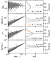 |
Fig. 1. Magneticum mass-observable relation for Euclid-like derived quantities. The left column shows scaling relations, relative fit (solid grey line), and a corridor corresponding to one standard deviation (dashed grey line). The right column shows the residual PDF and scatter of log-residuals σln. We report the following properties: lensing concentration |


In the right panel of Fig. 1, we show the log-residual distribution for both low-mass halos (M < 2 × 10¹⁴ M⊙), high-mass halos (M > 2 × 10¹⁴ M⊙), and for the complete sample of the log-residuals, σln, i, defined as the logarithmic ratio between the i-th cluster property and the corresponding scaling relation value at its mass. In the second column, we also report the log-scatter σln defined here as the corresponding standard deviation of the log-residual, namely,
![$$ \begin{aligned} \sigma _{\rm ln} = \mathrm{E}\left[\left(\sigma _{\mathrm{ln},i} - \mathrm{E}\left[\sigma _{\mathrm{ln},i}\right]\right)^2\right]^{1/2}, \end{aligned} $$](/articles/aa/full_html/2025/03/aa51347-24/aa51347-24-eq20.gif)
where E is the expectation operator that averages over our catalogue data. We note that the concentration has a scatter of 0.45, which is higher than theoretical expectations (see e.g. Child et al. 2018). Throughout this paper, we aim to show that this is due to projection effects; in fact, the 3D concentration has a scatter of ≈0.33.
We note that our scatter in temperature exceeds that reported in the theoretical work published by Truong et al. (2018). We verified that if we compute mass-weighted temperature, which is known to behave very well in a power-law scaling relation, reveals a log scatter of 0.07. This is in agreement with their work. The additional scatter that we see may be due to different X-ray temperature computations (the cited authors used core-excised temperature, whereas we have taken the contribution of the core into account).
In Fig. 2, we show the mass-observable relations of quantities that could potentially be obtained from various multi-wavelength observations that could enrich studies based on Euclid-like data products: the integrated Compton-y parameter, gas mass, Mg, 500c, X-ray luminosity,  converted in the soft band of [0.5, 2] keV, and the temperature, T500c. We decided to plot the X-ray luminosity, gas mass, and temperature within r500c because this radius is typically used in various X-ray observations (see e.g. Vikhlinin et al. 2006; Sun et al. 2009).
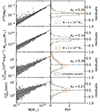 |
Fig. 2. Same as Fig. 1, but for the following multi-wavelength observable properties: Projected integrated Compton-y parameter Y2D (first row), the 3D gas mass Mg, 500c (second row), the projected X-ray luminosity in the soft band (in range [0.5, 2] keV) |


The typical Euclid cluster cosmology analysis will therefore rely on mass-observable relations calibrated within r200c (e.g. richness, weak-lensing mass), and follow-up observations calibrated within r500c (e.g. X-ray and SZ mass-proxies). Thus, we must consider the covariance between observable properties extracted at different radii.
Finally, we note that generally, X-ray observations are expected to align more closely with the 3D mass rather than the projected one (Ettori et al. 2013), although several details adopted to analyse the X-ray observations (e.g. including masking of substructures, de-projection procedures, etc.) can significantly impact the final result. These choices critically depend on the quality of the observations themselves. Dedicated mocks will thus be required to properly consider all these effects and, thus, they are beyond the purpose of this work. For simplicity, in this work, we consider an X-ray-derived gas mass as close to Mg, while an SZ-derived gas mass closer to  .
.
3. Projection effects
The main objective of this work is to disentangle the amount of scatter and skewness in scaling relations that is purely due to projection effects. We note that the observational data are also affected by measurement errors that we have not tackled in this work (e.g. the Poisson error of the limited number of galaxies used to infer the richness). In this section, we discuss the scatter and skewness of mass-observable relation qualitatively and limit the discussion to the data at a redshift of z = 0.24. We made this choice because we have a larger sample of galaxy clusters and the results are qualitatively similar to the ones at z = 0.9. We stress that we leave the quantitative discussion of the scatter and correlation coefficients for both redshifts on Sect. 5.
To assess the role of projection effects, Fig. 3 reports the 3D and 2D scatter of our cluster properties. In the left panel of Fig. 3, we show the value of the scatter (see Eq. 9) of log-residuals σln for all our mass-observable relations. In the shaded region, we also report the values computed within r500c for the X-ray luminosity, gas mass, and temperature values because this is the characteristic overdensity used in X-ray analyses.
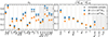 |
Fig. 3. Scatter of our mass-observable relations, paired with their projected version: concentration, integrated Compton-y parameter, gas mass, NFW mass, richness, stellar mass, X-ray luminosity, and temperature, within a radius of r200c; the grey band reports the gas mass, X-ray luminosity, and temperature within r500c. The left panel reports the fractional scatter of both 3D and 2D quantities. Each dotted vertical line separates the regions that report a given quantity and its 2D version. The right panel reports the contribution of projection effects. Points are coloured by their mass range as in Fig. 1, blue inverted triangles represent the low mass bin, orange up-triangles represent the high mass bin, and grey crosses represent the complete sample. Note: we lack the value of projection effects for LX, 500c (see discussion). Points are ordered according to the value of the second panel. Error bars are computed using the jackknife method. |
For each observable, we report (with different symbols) in Fig. 3 both the scatter of the complete sample as well as the one of two separate mass ranges of 1014 < M < 2 × 10¹⁴ M⊙ and M > 2 × 10¹⁴ M⊙ respectively. We note that the lower-mass bin (M < 2 × 10¹⁴ M⊙) is the one with the largest scatter because, for a given external object in the line-of-sight (LoS), the profile of a small cluster will be more perturbed with respect to a cluster.
In the left panel of Fig. 3, we see that some quantities have a low scatter in the 3D space and do gain a large amount of scatter once they are seen in projection. To better quantify what is the actual impact of projection effects, in the right panel of Fig. 3, we present the metric  . This metric shows that the quantities that are most affected by projection effects are the weak lensing concentration, integrated Compton-y parameter, gas mass, and NFW profile lensing mass. This is expected as all these observable properties (except for weak lensing concentration and X-ray luminosity) scale linearly with the respective observable mass. Further, we note that the scatter in the richness agrees to the theoretical predictions from Castignani & Benoist (2016).
We observe that X-ray luminosity and temperature are the least affected by projection effects. This is attributed to the fact that X-ray luminosity is contingent upon the square of gas density, thereby being primarily influenced by the most bright regions within an image. Similarly, the temperature is predominantly influenced by the innermost regions of a cluster. We note that we lack the value of projection effects for LX, 500c because the 2D scatter is slightly smaller than the 3D one. This happened because projection effects impact under-luminous halos more strongly than overly luminous halos (at a fixed mass bin), with the consequence of the projected X-ray luminosity having a higher normalisation and a lower scatter (see Fig. B.4).
Some mass-observable relations have a large skewness, to aid observational works in modelling these relations, we will estimate their skewness. Therefore, we also quantify deviations of residuals from a symmetrical distribution by means of the Fisher-Pearson coefficient of skewness, m3/m23/2, where mk is the sample kth central moment6. We report its dependency on projection effects in Fig. 4, showing that the properties whose skewness is most impacted by projection effects are the integrated Compton-y parameter, the gas mass, and the lensing NFW mass. We also notice that some scaling relation residuals move from having a negative skewness (for the NFW concentration, e.g. due to un-relaxed and merging clusters) to a positive one once projection effects are taken into account (i.e. from an asymmetry towards negative residuals towards an asymmetry towards positive residuals).
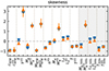 |
Fig. 4. Skewness parameters for our cluster properties. Data, line styles, and colours are as in Fig. 3. Error bars are computed using the jackknife method. |
To assess the impact of projection effects, we introduced a variable to quantify the amount of additional matter in the line of sight that can skew our observable properties. We define it as the ratio of the mass within the cylinder and the mass within a sphere, M2D/M, both of a radius of r200c, where the length of the cylinder is described in Sect. 2. We present the distribution of M2D/M in Fig. 5, where we can see that this quantity is strongly skewed and its median value is M2D/M ≈ 1.26 (note that for a NFW profile with c = 4, the corresponding analytical cylinder vs. spherical mass is 1.25). Although this quantity is not directly observable, we still use it to assess the contribution of LoS objects in the scatter of scaling relations. We note that besides objects in the LoS, different fitting procedures may impact the scatter of projection effects, as we will see in Sect. 4.
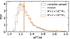 |
Fig. 5. Probability density distribution of M2D/M at different mass bins: for halos with M < 2 × 10¹⁴ M⊙ as a blue dotted line, for halos with M > 2 × 10¹⁴ M⊙ as a dashed orange line and for the complete sample as a grey solid line. For each mass bin, the vertical line represents the median values (note: the three lines are very close together). |
In Fig. 6, we show a random selection of clusters, ordered by decreasing M2D/M from left to right. Objects with high M2D/M (the objects in the left-most panels) include clusters that are merging, elongated, or in the LoS. In the rest of this paper, we refer to the objects with a M2D/M value greater than the median of the distribution 1.26 as having LoS excess.
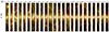 |
Fig. 6. Projected maps along a cylinder of length 23 Mpc, with radius r200c and centred on a random sample of our galaxy clusters, ordered by their M2D/M (over-plotted above each map) values decreasing from left to right. The pixel red, green, and blue channels are used as follows: the red channel maps the gas projected mass, the green channel maps the dark matter projected mass, and the blue channel maps the stellar projected mass. Columns widths are proportional to the cluster radii. |
To study the impact of projection effects in scaling relations, in Fig. 7, we show the scaling relations of the following projected quantities: richness, integrated Compton-y parameter, lensing mass, and concentrations, which are the ones that are most affected by projection effects. We colour-code these points by M2D/M and focus on a narrow mass range of M ∈ [1, 2]×1014 M⊙ to better visualise how LoS excess impacts these scaling relations. On the left column, we visually depict the fact that (with the exception of the concentration), they are strongly correlated with M2D/M, as the upper points of the scatter plot tend to have higher values of M2D/M.
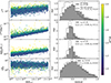 |
Fig. 7. Impact of LoS contamination in scaling relations. We show halo properties as a function of halo mass M in the left column, and colour-coded by the fractional amount of mass in a cylinder (M2D/M), and the residuals PDFs in the right column (grey shaded histogram). Rows correspond to richness, the integrated Compton-y parameter, lensing mass, and lensing concentration. We also show the residuals of a subset of halos with low LoS contamination (in particular M2D/M < 1.26, dashed line histogram). Each panel reports the scatter of the residuals σ and the mean μ of the low LoS residuals. |
We quantified this finding in the right column by comparing the residual distributions (of the power-law fit over the complete mass range presented in Sect. 2.2) of the complete sample with the distribution of objects with low LoS contamination only (we adopted the criteria of M2D/M < 1.26 as the median of the M2D/M distribution, shown in Fig. 5). We then reported the respective scatter, σ, and average value, μ, of the residual distributions (for the complete sample we have that μ = 0). Except for the concentration, residuals of halos with low M2D/M (see dashed histogram) significantly shift towards negative values of μ and σ. For instance, when we consider only objects with a low LoS excess, the scatter of Y2D decreases from 0.35 down to 0.11, while the  scatter goes from 0.23 to 0.9. The lensing mass is, in fact, generally known to be affected by projection effects (Meneghetti et al. 2014; Euclid Collaboration 2024).
In this paper, we refer to projection effects as all effects that take place when going from 3D to projection; they include both LoS effects and model uncertainties. This definition becomes relevant when dealing with concentration, which is impacted not only by LoS objects, but also by the NFW profile fitting procedure. We stress that in Fig. 3 we proved that our projected concentration is actually highly impacted by projection effects, yet only weakly affected by LoS effects. We show in the next section the reason for concentration being strongly affected by projection effects is that their reduced shear profile deviates strongly from the one produced by NFW profile (see, e.g. Ragagnin et al. 2021), which is used to reconstruct the reduced shear profile.
To conclude this part of the paper, we go on to study how correlations between cluster observable properties can be affected by projection effects. To this end, we take the case of a possible hot- versus cold-baryon correlation by studying the stellar mass versus integrated Compton-y parameter (as the latter should strongly correlate with the gas mass). In Fig. 8, we show the integrated Compton-y parameter scaling relation, colour-coded by stellar mass for the 3D quantities (top panel) and projected quantities (bottom panel).
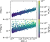 |
Fig. 8. Integrated Compton-y parameter vs halo mass, colour-coded by a stellar mass fraction. The top panel shows quantities computed within a sphere of radius r200c, while in the bottom panel, they are computed within a cylinder (of radius r200c and length 23 Mpc as already presented in Sect. 2). We limit the plot in the mass range M ∈ [1, 2]×1014 M⊙. |
Examining the correlations at a constant halo mass among the computed quantities within spheres (as depicted in the top panel of Fig. 8), we find no discernible weak anti-correlation between stellar mass and the integrated Compton-y parameter (which is defined in Sect. 5). Conversely, when investigating the properties in the projected space, a more pronounced correlation becomes evident. This implies that projection effects can strongly impact the correlation between observable properties. While this analysis is purely qualitative, we go on to quantify the impact of these projection effects in Sect. 5, where we compute the correlation coefficients for both 3D quantities and 2D quantities.
4. Projection effects on lensing concentration
As we found in the previous section, projection effects significantly increase the scatter and skewness in the scaling of lensing concentration with mass. However, this scatter increase is not related to external objects along the LoS. Next, we can assess if the high scatter of lensing concentration is due to deviations of the reduced shear profile from the one induced by an NFW profile.
In this work, we do not delve into the origin of this deviation as it falls beyond the scope of this paper. Such deviation may arise due to halo elongations, suggesting that alternative profiles such as truncated NFW profiles may better suit galaxy clusters (Oguri & Hamana 2011). Alternatively, it could stem from the expectation that the NFW profile is intended to describe stacked halos rather than individual objects. Our focus in this paper is to understand the impact of assuming an NFW profile for each of our halos. We emphasise that these NFW deviations only affect weak lensing signal reconstruction, as the NFW profile is highly effective in recovering halo mass in 3D.
To study deviations from the NFW profile of halos we fit a generalised NFW profile (Nagai et al. 2007); hereafter, gNFW, in spherical coordinates over the same radial range as our previous NFW profile (described in Sect. 2.1), where the density profile ρgNFW(r) is defined as
Here, γ and β are respectively the internal and external log-slopes of the total matter density profiles. The case γ = 1 and β = 3 produces the NFW profile as in Eq. (4). We note that the Nagai et al. (2007) gNFW profile also depends on the parameter α that we fixed to α = 1 in this work to explore internal and external log-slope variations only.
We present the PDF for the gNFW profile parameters γ and β in Fig. 9, where the fit was performed in 3D with a flat priors for γ ∈ [0, 3] and β ∈ [0, 6]. The data points are colour-coded according to the variable M, revealing no discernible strong trend with respect to the fitted parameters. For 19% of the objects, the resulting best-fit parameters hit the boundaries of hard-cut priors. Upon visual inspection, these objects are characterised by a very steep matter density profile at large cluster-centric distances, possibly suggesting that a truncated NFW profile might be a better model choice. As our objective is to examine the effects of deviations from the generalised NFW profile, we omitted these objects from the subsequent analysis in this section. Given the substantial deviation of these objects from NFW profile, they could potentially offer additional insights for our analyses. However, incorporating them would necessitate the use of a profile more general than Eq. (10). Therefore, we excluded them in order to make our analysis clearer.
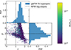 |
Fig. 9. Probability density distribution of the parameters γ (inner slope, upper panel) and β (outer slope, right panel) of Eq. (10) of the successful gNFW profile fits. The central panel shows the scatter plot between the two parameters colour-coded by M. The dotted lines show the NFW parameters γ = 1 and β = 3. |
We observe that the external logslope of Magneticum profiles appears to be slightly flatter than −3. While we emphasise that this discrepancy does not affect the accurate recovery of mass and concentration parameters in 3D NFW fits (such fits can still yield precise estimates of halo mass and concentrations). However, these deviations in the NFW profiles may affect the reduced shear fit, particularly when observed over large radii (noting that in this work, we use 3 Mpc).
Furthermore, we observe a degeneracy between the β and γ parameters, indicating that our profiles deviating from NFW profile tend to exhibit a flatter profile compared to NFW profile (as illustrated in Fig. A.1). However, investigating this discrepancy is beyond the scope of this paper, as the internal log slope of clusters is not currently captured by existing weak lensing studies.
In Fig. 10, we plot the values of concentration and mass obtained from reduced shear fit, divided by the corresponding 3D quantities and colour-coded by the external 3D gNFW slope β for our intermediate redshift halos. As we can see, halos with large values of β have a projected concentration that is significantly higher than the 3D one (see upper panel). In Appendix A, we report the example of a simulated halo with low LoS excess (see Fig. A.1) and an analytical one (see Fig. A.2), both with a flat external log-slope. We show how the under-estimation of the concentration is caused by the fact that the NFW profile fit on the reduced shear is disproportionately weighting the external part of the profile, which makes it deviate from an NFW profile.
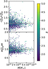 |
Fig. 10. Ratio between 2D NFW profile fit parameters and 3D parameters for halos with a successful 3D gNFW profile fit. Upper panel: Ratio between concentrations. Lower panel: Ratio between halo masses. Points are colour-coded by the external log-slope β of the 3D fit of gNFW. |
We show the concentration residual distribution in Fig. 11 and report their scatter. We note that the projected concentration scatter is not affected by external material along the LoS (where the dashed line and shaded histograms match). However, if we restrict our sample to objects having NFW-like profile log-slopes (we use the criteria of 2.8 < β < 3.2 and 0.8 < γ < 1.2), then the scatter distribution changes drastically. The concentration residuals decrease from 0.43 to 0.38, and the residuals shift towards higher values, suggesting that these objects are more relaxed. This effect is widely known, as studied, for instance, in Macciò et al. (2007).
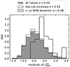 |
Fig. 11. Residuals of lensing concentrations with respect to the power-law fit. As in Fig. 7, the dashed line histogram indicates the residuals for objects with low LoS effects (low value of M2D/M). The solid line histogram contains the additional constraints of halos with β and γ parameters close to the ones of an NFW profile (2.8 < β < 3.2 and 0.8 < γ < 1.2). Each histogram label reports the scatter σ of the residuals. |
We also show how the external log-slope of the halo profile affects the lensing reconstruction by plotting the ratio between the projected and 3D concentration (i.e.  ) value versus the 3D log-slope β in the narrow mass bin of M ∈ [1, 2]×1014 M⊙ in Fig. 12. We find a positive correlation coefficient of ≈0.28, in agreement with a shift of residuals given in Fig. 11.
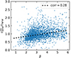 |
Fig. 12. Scatter plot of ratio between 2D concentration and 3D concentration against β, namely, the outer slope of Eq. (10), of good 3D gNFW profile fits in a narrow mass range of M ∈ [1, 2]×1014 M⊙. We also report the correlation coefficient. |
5. Correlations between properties
In the last sections of this paper, we describe our investigation of the origin of the impact of projection effects in the scatter and skewness of observable properties. We go on to quantify how projection effects impact the correlation between observable properties. To this end, we quantified the Pearson correlation coefficients between their log-residuals (as defined in Sect. 2.2). We adopted the standard error associated with the Pearson coefficient, ρ, as derived from two normal distributions, given by  (see Eqs. 12–93 in Pugh & Winslow 1966), where N represents the number of objects. This corresponds to a maximum error of 0.015 (for ρ = 0) for the sample size at z = 0.24 and a maximum error of 0.028 for the sample size at z = 0.90. It is worth noting that in the correlation coefficient matrices generated in subsequent analyses, we only coloured values with correlation coefficients of |ρ|> 0.3, with an aim to highlight strongly correlating properties. We defined a mild correlation as 0.2 < |ρ|< 0.3, as we chose to exercise caution. Correlation coefficients with |ρ|< 0.1 were disregarded.
5.1. Analysis at z = 0.24
In this section, we focus on the halos at intermediate redshift at z = 0.24. In Fig. B.1, we show the correlation coefficient matrix between log-residuals at fixed halo mass of our projected observable both from Euclid-like data (lensing concentration, lensing mass, richness, and stellar mass, respectively) and possible outcomes from multi-wavelength observations (integrated Compton-y parameter, gas mass, X-ray luminosity, and temperature) for intermediate-redshift objects.
In the lower triangle, we present scatter plots alongside the slope derived from the correlation coefficient. This visualisation allows for the identification of instances where the correlation coefficient slope accurately captures the trend of the residuals. Typically, this alignment occurs for quantities that exhibit strong correlation coefficients. For example, our data points show a robust correlation between certain hot baryon tracers ( and Y2D), some cold baryon components (n2D and M⋆2D), and weak lensing mass,
  . The underlying reason for these strong correlations lies in projection effects: the greater the amount of matter along the line of sight, the higher the observed values. We demonstrate this further in the subsequent section by presenting the correlation coefficient matrix for 3D quantities, where many of these correlations diminish. This can be anticipated by observing that Lx2D and
  do not exhibit this positive trend of correlations.
Notably, we observe that the correlation between richness and stellar mass (ρ = 0.48) is not exceptionally high. Moreover, the stellar mass appears to be more influenced by projection effects compared to richness (evident in their correlations with  , where they exhibit ρ = 0.69 and ρ = 0.42, respectively). We can speculate on two potential causes: firstly, unlike stellar mass, our richness computation incorporates some observationally-motivated background subtraction; alternatively, since stellar mass encompasses all stellar particles (while richness involves a luminosity-motivated galaxy stellar-mass cut), it is plausible that small subhalos are influencing the projected stellar mass.
We note that the concentration is anti-correlated with the gas-mass (and integrated Compton-y parameter). This is in agreement with recent analyses of simulations. In fact, richness at fixed mass is anti-correlated with concentration (Bose et al. 2019), while low concentration is an index of the system being perturbed (Ludlow et al. 2012) and un-relaxed systems tend to be gas-rich (Davies et al. 2020). We refer to Ragagnin et al. (2022a) for a more comprehensive study on low luminous groups. Moreover, at fixed halo mass, the lensing mass correlates strongly with total projected stellar mass (ρ = 0.69) and projected gas mass (ρ = 0.59), which may be due to the fact that both correlate strongly with LoS contamination. The same holds for the correlation among richness, gas mass, and stellar mass. This is due to projection effects, where LoS excess amplifies all these quantities, as discussed in Sect. 2.2. We note that the 2D lensing mass and projected X-ray luminosity have a slightly positive (ρ = 0.20) correlation, in agreement with the observational work of Sereno et al. (2020).
In Fig. B.2, we show the covariance matrix of non-projected quantities for intermediate redshift objects. We see that (as opposed to what is seen Fig. B.1), the 3D covariance matrix shows a mild yet negative covariance between gas mass and stellar mass (ρ = −0.24), along with a positive correlation between richness and gas mass (ρ = 0.23) because most of their correlations in the projection are due to the line of sight excess, which significantly increases the values of the gas mass, the richness, and the stellar mass. In Fig. B.3, we report the correlation matrix as in Fig. B.1 where we present X-ray luminosity, gas mass, and temperature, as computed within r500c, which shows an anti-correlation between the gas mass and the concentration residuals (ρ = −0.14), which is significantly lower than the one found in Figs. B.1 and B.2 (ρ is equal to −0.26 and −0.34, respectively). One possibility is that this change in sign of the correlation is caused by the fact that mixing overdensities (concentration is within Δc = 200 and gas-mass is within Δc = 500) does introduce an additional correlation with the sparsity (Balmès et al. 2014; Corasaniti et al. 2022), which itself is correlated with the concentration (see Appendix B).
For completeness, we report the correlation coefficient matrix and the scatter of log-residuals of all quantities in Table B.1. There, we also added the core-excised projected X-ray luminosity  , as it is typically used in X-ray-based observational studies. Thus, we can see that the scatter and most of the correlation coefficients are smaller than
  , while the correlations with the concentration and gas mass increase. We note that we have not reported the 3D NFW mass (MNFW) because it has an extremely low intrinsic scatter σln(MNFW)≈0.01 and its correlation coefficients are not meaningful.
5.2. Analysis at z = 0.9
In this section, we focus on observational property covariance matrixes of our halos at z = 0.9. At this redshift, we computed projected quantities within a cylinder depth of 35 Mpc to retain the same relative ratio as the photo-z uncertainty of the low-redshift analysis (it scales with 1 + z). With respect to the cylinder used to integrate ΔΣgt, we re-scaled so as to keep it constant in comoving units with the low-redshift analyses. We re-scaled the 3D NFW profile minimum radius to 40 kpc while we kept the maximum radius at r200c. With respect to the radial range of the lensing fit, we re-scaled it with H−2/3(z); thus, it was carried out in the range of [234, 2300] kpc.
We stress that we do not model observational uncertainty. Therefore, the decrease in background source count with redshift does not impact our best fits. However, it still impacts the fact that we weigh external radial bins more than the internal ones. We report the values of the scatter and the projection contribution at z = 0.9 in Fig. B.6, while we report the log-residuals and the skewness for each property in Fig. B.7.
In particular, the quantities most affected by projection effects are the lensing mass and concentration, whereas the temperature is the lowest. These results are qualitatively similar to the low redshift analyses, with the Compton-Y parameter and gas mass being slightly less affected by projection effects. We note that since the virial radius is smaller at higher redshift values, our radial range of the reduced shear is closer to the NFW scale radius; therefore, the weak lensing reconstruction is more effective in capturing the scale radius and more sensitive to deviations from an NFW profile. As a consequence, we found that the increase of scatter going from cNFW to  compared to the low redshift analyses.
We report the correlation coefficient matrix and the scatter log residuals of the quantities at z = 0.9 in Table B.2. We corroborate the tables with the scatter and skewness analyses at z − 0.9 in Figs. B.6 and B.7 respectively. As for the case at z = 0.24, we note that we do not report the 3D NFW mass (MNFW) because it has an extremely small intrinsic scatter of 0.01; thus, its correlation coefficients have no impact in our study.
6. Conclusions
In this work, we have analysed a number of galaxy clusters from Magneticum hydrodynamic simulation Box2b/hr. We carried out our study in a mass range, tailored for Euclid-like data products (see Sartoris et al. 2016; Euclid Collaboration 2019); namely, with a mass of M200c > 1014 M⊙. To this end, we computed properties that could come from Euclid catalogues of galaxy clusters, such as richness, stellar mass, and lensing masses and concentration, along with plausible properties coming from multi-wavelength studies, such as X-ray luminosity, integrated Compton-y parameter, gas mass, and temperature. All these properties were computed both within a sphere and within a cylinder (both with radius r200c) to account for projection effects. Our study considers the remarkable capabilities of Euclid photo-z measurements in identifying interlopers. However, their importance decreases significantly at scales as small as a few tens of Mpc. This depth is still enough to contain multiple halos along the LoS. Hence, we studied the projection effects on a scale that is significantly smaller than the Euclid photo-z uncertainty. We then studied how the scatter and skewness change when we are measuring quantities in 3D space or in projection. We summarise our findings below.
-
The properties that are most affected by projection effects are the mass and concentration from lensing, the integrated Compton-y parameter, and the gas mass. In contrast, the temperature and X-ray luminosity are the quantities least affected by projection effects.
-
In both redshift slices (z = 0.24 and z = 0.9), the influence of LoS effects is substantial and potentially leads to a spurious correlation between gas and stellar masses. These projection effects have the capacity to markedly enhance correlations between gas and stellar mass (they go from a negative value of −0.24 to a significantly high value of 0.57), effectively masking the intrinsic underlying correlation (e.g. one driven by distinct accretion histories).
-
The lensing concentration, on the other hand, is mainly affected by the fact that the profile outskirts of reduced shear deviate from the one coming from an NFW profile (which is the profile typically used in WL analyses). We found that deviations from an ideal NFW profile increase the skewness from 0.6 to 2.5 and increase the scatter of log-residuals from 0.33 (in agreement with theoretical works) up to 0.46.
The analysis presented here has been carried out using a single suite of hydrodynamic simulations. Regarding weak lensing masses and concentration, since in this work, we did not consider the profile noise due to the finite number of background galaxies. Future studies are needed to improve our estimations.
Some works have shown that both scatter and correlation coefficients vary between cosmological simulations with different cosmologies (Ragagnin et al. 2023), the presence of feedback schemes (Stanek et al. 2010), and different cosmological simulation suite in the market (see Fig. 7 in Anbajagane et al. 2020). So, while simulations can provide directions on how to model correlation coefficients, it is possible that when using simulated data, we need to allow for variation due to the different baryon physics. Further studies that assess the role of baryon physics may also help reduce recent tensions between simulations and observations (see e.g. Ragagnin et al. 2022b).
Furthermore, when striving for even more precise results, it is important to acknowledge that mass-observable relations are not exact power laws. Therefore, employing more generic fitting techniques, such as a running median, could yield improvements. Additionally, there is room for enhancement in how we compute correlation coefficients in future studies. One potential approach could involve simultaneously fitting both the mass-observable relation scatter and the correlation coefficients by maximising multi-variate likelihoods. We anticipate that future studies combining Euclid data with multi-wavelength observations may encounter challenges in shedding light on residual correlations, which are puzzling at present and primarily dominated by projection effects.
Data availability
Raw simulation data were generated at C2PAP/LRZ cosmology simulation web portal https://c2papcosmosim.uc.lrz.de/. Derived data supporting the findings of this study are available from the corresponding author AR on request.
Note that Euclid richness will be based on detection algorithms such as AMICO (Bellagamba et al. 2018) or PZWav, which may provide similar or different removal for projection effects. However, we do not have Magneticum Box2b light cones to feed to these algorithms. We stress that our richness computation anyway is very close to what is used in other observational works as Andreon et al. (2016).
We credit Biffi et al. (2017) and Truong et al. (2018) for the routines and cooling tables we used.
Acknowledgments
We thank the anonymous referee for the useful comments. The Magneticum Pathfinder simulations were partially performed at the Leibniz-Rechenzentrum with CPU time assigned to the Project ‘pr86re’. AR and LM acknowledge support from the grant PRIN-MIUR 2017 WSCC32 and acknowledges the usage of the INAF-OATs IT framework (Taffoni et al. 2020; Bertocco et al. 2020), and the space filling curve improvement on Gadget3 (Ragagnin et al. 2016). Antonio Ragagnin thanks Veronica Biffi and Elena Rasia for the X-ray computation routines and tables. KD acknowledges support by the COMPLEX project from the European Research Council (ERC) under the European Union’s Horizon 2020 research and innovation program grant agreement ERC-2019-AdG 882679. LM acknowledges the financial contribution from the grant PRIN-MUR 2022 20227RNLY3 “The concordance cosmological model: stress-tests with galaxy clusters” supported by Next Generation EU. CG and LM acknowledge support from the grant ASI n.2018-23-HH.0. AR and CG acknowledge funding from INAF theory Grant 2022: Illuminating Dark Matter using Weak Lensing by Cluster Satellites, PI: Carlo Giocoli. SB acknowledges partial financial support from the INFN InDark grant. AMCLB was supported by a fellowship of PSL University hosted by the Paris Observatory. We used the package colossus (see Diemer 2018) for computing Σ and ΔΣ as expected from NFW profiles. AR and FC acknowledge co-funding by the European Union – NextGenerationEU within PRIN 2022 project n.20229YBSAN – Globular clusters in cosmological simulations and in lensed fields: from their birth to the present epoch. The Euclid Consortium acknowledges the European Space Agency and a number of agencies and institutes that have supported the development of Euclid, in particular the Agenzia Spaziale Italiana, the Austrian Forschungsförderungsgesellschaft funded through BMK, the Belgian Science Policy, the Canadian Euclid Consortium, the Deutsches Zentrum für Luft-und Raumfahrt, the DTU Space and the Niels Bohr Institute in Denmark, the French Centre National d’Etudes Spatiales, the Fundação para a Ciência e a Tecnologia, the Hungarian Academy of Sciences, the Ministerio de Ciencia, Innovación y Universidades, the National Aeronautics and Space Administration, the National Astronomical Observatory of Japan, the Netherlandse Onderzoekschool 870 Voor Astronomie, the Norwegian Space Agency, the Research Council of Finland, the Romanian Space Agency, the State Secretariat for Education, Research, and Innovation (SERI) at the Swiss Space Office (SSO), and the United Kingdom Space Agency. A complete and detailed list is available on the Euclid website (www.euclid-ec.org).
References
- Abbott, T. M. C., Aguena, M., Alarcon, A., et al. 2020, Phys. Rev. D, 102, 023509 [Google Scholar]
- Allen, S. W., Evrard, A. E., & Mantz, A. B. 2011, ARA&A, 49, 409 [Google Scholar]
- Anbajagane, D., Evrard, A. E., Farahi, A., et al. 2020, MNRAS, 495, 686 [NASA ADS] [CrossRef] [Google Scholar]
- Andreon, S., & Moretti, A. 2011, A&A, 536, A37 [NASA ADS] [CrossRef] [EDP Sciences] [Google Scholar]
- Andreon, S., Dong, H., & Raichoor, A. 2016, A&A, 593, A2 [NASA ADS] [CrossRef] [EDP Sciences] [Google Scholar]
- Angelinelli, M., Ettori, S., Dolag, K., Vazza, F., & Ragagnin, A. 2022, A&A, 663, L6 [NASA ADS] [CrossRef] [EDP Sciences] [Google Scholar]
- Angelinelli, M., Ettori, S., Dolag, K., Vazza, F., & Ragagnin, A. 2023, A&A, 675, A188 [NASA ADS] [CrossRef] [EDP Sciences] [Google Scholar]
- Angulo, R. E., Zennaro, M., Contreras, S., et al. 2021, MNRAS, 507, 5869 [NASA ADS] [CrossRef] [Google Scholar]
- Arnaud, K. A. 1996, ASP Conf. Ser., 101, 17 [Google Scholar]
- Balmès, I., Rasera, Y., Corasaniti, P. S., & Alimi, J. M. 2014, MNRAS, 437, 2328 [CrossRef] [Google Scholar]
- Beck, A. M., Murante, G., Arth, A., et al. 2016, MNRAS, 455, 2110 [Google Scholar]
- Becker, M. R., & Kravtsov, A. V. 2011, ApJ, 740, 25 [NASA ADS] [CrossRef] [Google Scholar]
- Bellagamba, F., Roncarelli, M., Maturi, M., & Moscardini, L. 2018, MNRAS, 473, 5221 [NASA ADS] [CrossRef] [Google Scholar]
- Bertocco, S., Goz, D., Tornatore, L., et al. 2020, ASP Conf. Ser., 527, 303 [NASA ADS] [Google Scholar]
- Bhargava, S., Garrel, C., Koulouridis, E., et al. 2023, A&A, 673, A92 [NASA ADS] [CrossRef] [EDP Sciences] [Google Scholar]
- Biffi, V., Dolag, K., & Böhringer, H. 2013, MNRAS, 428, 1395 [Google Scholar]
- Biffi, V., Planelles, S., Borgani, S., et al. 2017, MNRAS, 468, 531 [Google Scholar]
- Bocquet, S., Saro, A., Dolag, K., & Mohr, J. J. 2016, MNRAS, 456, 2361 [Google Scholar]
- Bocquet, S., Dietrich, J. P., Schrabback, T., et al. 2019, ApJ, 878, 55 [Google Scholar]
- Bocquet, S., Heitmann, K., Habib, S., et al. 2020, ApJ, 901, 5 [Google Scholar]
- Bocquet, S., Grandis, S., Bleem, L. E., et al. 2024, Phys. Rev. D, 110, 083510 [NASA ADS] [CrossRef] [Google Scholar]
- Bose, S., Eisenstein, D. J., Hernquist, L., et al. 2019, MNRAS, 490, 5693 [CrossRef] [Google Scholar]
- Boylan-Kolchin, M., Springel, V., White, S. D. M., Jenkins, A., & Lemson, G. 2009, MNRAS, 398, 1150 [Google Scholar]
- Castignani, G., & Benoist, C. 2016, A&A, 595, A111 [NASA ADS] [CrossRef] [EDP Sciences] [Google Scholar]
- Child, H. L., Habib, S., Heitmann, K., et al. 2018, ApJ, 859, 55 [NASA ADS] [CrossRef] [Google Scholar]
- Contreras-Santos, A., Buitrago, F., Knebe, A., et al. 2024, A&A, 690, A109 [NASA ADS] [CrossRef] [EDP Sciences] [Google Scholar]
- Corasaniti, P. S., Le Brun, A. M. C., Richardson, T. R. G., et al. 2022, MNRAS, 516, 437 [NASA ADS] [CrossRef] [Google Scholar]
- Costanzi, M., Rozo, E., Simet, M., et al. 2019, MNRAS, 488, 4779 [NASA ADS] [CrossRef] [Google Scholar]
- Cui, W., Dave, R., Knebe, A., et al. 2022, MNRAS, 514, 977 [NASA ADS] [CrossRef] [Google Scholar]
- Davies, J. J., Crain, R. A., Oppenheimer, B. D., & Schaye, J. 2020, MNRAS, 491, 4462 [NASA ADS] [CrossRef] [Google Scholar]
- Davis, M., Efstathiou, G., Frenk, C. S., & White, S. D. M. 1985, ApJ, 292, 371 [Google Scholar]
- Diemer, B. 2018, ApJS, 239, 35 [NASA ADS] [CrossRef] [Google Scholar]
- Dolag, K., Borgani, S., Murante, G., & Springel, V. 2009, MNRAS, 399, 497 [Google Scholar]
- Dolag, K., Gaensler, B. M., Beck, A. M., & Beck, M. C. 2015, MNRAS, 451, 4277 [NASA ADS] [CrossRef] [Google Scholar]
- Dolag, K., Komatsu, E., & Sunyaev, R. 2016, MNRAS, 463, 1797 [Google Scholar]
- Ettori, S., Donnarumma, A., Pointecouteau, E., et al. 2013, Space Sci. Rev., 177, 119 [Google Scholar]
- Euclid Collaboration (Adam, R., et al.) 2019, A&A, 627, A23 [NASA ADS] [CrossRef] [EDP Sciences] [Google Scholar]
- Euclid Collaboration (Blanchard, A., et al.) 2020a, A&A, 642, A191 [NASA ADS] [CrossRef] [EDP Sciences] [Google Scholar]
- Euclid Collaboration (Desprez, G., et al.) 2020b, A&A, 644, A31 [EDP Sciences] [Google Scholar]
- Euclid Collaboration (Ajani, V., et al.) 2023, A&A, 675, A120 [NASA ADS] [CrossRef] [EDP Sciences] [Google Scholar]
- Euclid Collaboration (Giocoli, C., et al.) 2024, A&A, 681, A67 [NASA ADS] [CrossRef] [EDP Sciences] [Google Scholar]
- Euclid Collaboration (Mellier, Y., et al.) 2025, A&A, in press, https://doi.org/10.1051/0004-6361/202450810 [Google Scholar]
- Fabjan, D., Borgani, S., Tornatore, L., et al. 2010, MNRAS, 401, 1670 [Google Scholar]
- Farahi, A., Mulroy, S. L., Evrard, A. E., et al. 2019, Nat. Commun., 10, 2504 [NASA ADS] [CrossRef] [Google Scholar]
- Ferland, G. J., Korista, K. T., Verner, D. A., et al. 1998, PASP, 110, 761 [Google Scholar]
- Fischer, M. S., Kasselmann, L., Brüggen, M., et al. 2024, MNRAS, 529, 2327 [NASA ADS] [CrossRef] [Google Scholar]
- Ghirardini, V., Bulbul, E., Artis, E., et al. 2024, A&A, 689, A298 [NASA ADS] [CrossRef] [EDP Sciences] [Google Scholar]
- Giocoli, C., Tormen, G., & van den Bosch, F. C. 2008, MNRAS, 386, 2135 [NASA ADS] [CrossRef] [Google Scholar]
- Giodini, S., Lovisari, L., Pointecouteau, E., et al. 2013, Space Sci. Rev., 177, 247 [Google Scholar]
- Hirschmann, M., Dolag, K., Saro, A., et al. 2014, MNRAS, 442, 2304 [Google Scholar]
- Hoekstra, H. 2003, MNRAS, 339, 1155 [NASA ADS] [CrossRef] [Google Scholar]
- Hoekstra, H., Mahdavi, A., Babul, A., & Bildfell, C. 2012, MNRAS, 427, 1298 [NASA ADS] [CrossRef] [Google Scholar]
- Hudson, D. S., Mittal, R., Reiprich, T. H., et al. 2010, A&A, 513, A37 [NASA ADS] [CrossRef] [EDP Sciences] [Google Scholar]
- Komatsu, E., Smith, K. M., Dunkley, J., et al. 2011, ApJS, 192, 18 [Google Scholar]
- Kravtsov, A. V., & Borgani, S. 2012, ARA&A, 50, 353 [Google Scholar]
- Lima, M., & Hu, W. 2005, Phys. Rev. D, 72, 043006 [NASA ADS] [CrossRef] [Google Scholar]
- Ludlow, A. D., Navarro, J. F., Li, M., et al. 2012, MNRAS, 427, 1322 [NASA ADS] [CrossRef] [Google Scholar]
- Macciò, A. V., Dutton, A. A., van den Bosch, F. C., et al. 2007, MNRAS, 378, 55 [Google Scholar]
- Maturi, M., Bellagamba, F., Radovich, M., et al. 2019, MNRAS, 485, 498 [Google Scholar]
- McClintock, T., Varga, T. N., Gruen, D., et al. 2019, MNRAS, 482, 1352 [Google Scholar]
- Melchior, P., Suchyta, E., Huff, E., et al. 2015, MNRAS, 449, 2219 [NASA ADS] [CrossRef] [Google Scholar]
- Meneghetti, M., Rasia, E., Merten, J., et al. 2010, A&A, 514, A93 [NASA ADS] [CrossRef] [EDP Sciences] [Google Scholar]
- Meneghetti, M., Rasia, E., Vega, J., et al. 2014, ApJ, 797, 34 [Google Scholar]
- Nagai, D., Kravtsov, A. V., & Vikhlinin, A. 2007, ApJ, 668, 1 [Google Scholar]
- Navarro, J. F., Frenk, C. S., & White, S. D. M. 1997, ApJ, 490, 493 [Google Scholar]
- Oguri, M., & Hamana, T. 2011, MNRAS, 414, 1851 [NASA ADS] [CrossRef] [Google Scholar]
- Okabe, N., Zhang, Y. Y., Finoguenov, A., et al. 2010, ApJ, 721, 875 [NASA ADS] [CrossRef] [Google Scholar]
- Pacaud, F., Pierre, M., Adami, C., et al. 2007, MNRAS, 382, 1289 [Google Scholar]
- Pires, S., Vandenbussche, V., Kansal, V., et al. 2020, A&A, 638, A141 [NASA ADS] [CrossRef] [EDP Sciences] [Google Scholar]
- Pratt, G. W., Arnaud, M., Biviano, A., et al. 2019, Space Sci. Rev., 215, 25 [Google Scholar]
- Puddu, E., & Andreon, S. 2022, MNRAS, 511, 2968 [NASA ADS] [CrossRef] [Google Scholar]
- Pugh, E., & Winslow, G. 1966, The Analysis of Physical Measurements (Addison-Wesley) [Google Scholar]
- Ragagnin, A., Tchipev, N., Bader, M., Dolag, K., & Hammer, N. J. 2016, in Advances in Parallel Computing, Volume 27: Parallel Computing: On the Road to Exascale, eds. G. R. Joubert, H. Leather, M. Parsons, F. Peters, & M. Sawyer (IOP Ebook), 411 [Google Scholar]
- Ragagnin, A., Dolag, K., Biffi, V., et al. 2017, Astron. Comput., 20, 52 [Google Scholar]
- Ragagnin, A., Dolag, K., Moscardini, L., Biviano, A., & D’Onofrio, M. 2019, MNRAS, 486, 4001 [Google Scholar]
- Ragagnin, A., Saro, A., Singh, P., & Dolag, K. 2021, MNRAS, 500, 5056 [Google Scholar]
- Ragagnin, A., Andreon, S., & Puddu, E. 2022a, A&A, 666, A22 [NASA ADS] [CrossRef] [EDP Sciences] [Google Scholar]
- Ragagnin, A., Meneghetti, M., Bassini, L., et al. 2022b, A&A, 665, A16 [NASA ADS] [CrossRef] [EDP Sciences] [Google Scholar]
- Ragagnin, A., Fumagalli, A., Castro, T., et al. 2023, A&A, 675, A77 [NASA ADS] [CrossRef] [EDP Sciences] [Google Scholar]
- Ragagnin, A., Meneghetti, M., Calura, F., et al. 2024, A&A, 687, A270 [NASA ADS] [CrossRef] [EDP Sciences] [Google Scholar]
- Rozo, E., Wechsler, R. H., Rykoff, E. S., et al. 2010, ApJ, 708, 645 [Google Scholar]
- Saro, A., Liu, J., Mohr, J. J., et al. 2014, MNRAS, 440, 2610 [Google Scholar]
- Sartoris, B., Biviano, A., Fedeli, C., et al. 2016, MNRAS, 459, 1764 [Google Scholar]
- Schrabback, T., Bocquet, S., Sommer, M., et al. 2021, MNRAS, 505, 3923 [NASA ADS] [CrossRef] [Google Scholar]
- Sereno, M., Fedeli, C., & Moscardini, L. 2016, JCAP, 01, 042 [NASA ADS] [Google Scholar]
- Sereno, M., Umetsu, K., Ettori, S., et al. 2020, MNRAS, 492, 4528 [CrossRef] [Google Scholar]
- Singh, P., Saro, A., Costanzi, M., & Dolag, K. 2020, MNRAS, 494, 3728 [NASA ADS] [CrossRef] [Google Scholar]
- Smith, R. K., Brickhouse, N. S., Liedahl, D. A., & Raymond, J. C. 2001, ApJ, 556, L91 [Google Scholar]
- Sommer, M. W., Schrabback, T., Applegate, D. E., et al. 2022, MNRAS, 509, 1127 [Google Scholar]
- Sommer, M. W., Schrabback, T., Ragagnin, A., & Rockenfeller, R. 2024, MNRAS, 532, 3359 [NASA ADS] [CrossRef] [Google Scholar]
- Springel, V. 2005, MNRAS, 364, 1105 [Google Scholar]
- Springel, V., White, S. D. M., Jenkins, A., et al. 2005a, Nature, 435, 629 [Google Scholar]
- Springel, V., Di Matteo, T., & Hernquist, L. 2005b, MNRAS, 361, 776 [Google Scholar]
- Springel, V., White, S. D. M., Tormen, G., & Kauffmann, G. 2001, MNRAS, 328, 726 [Google Scholar]
- Stanek, R., Rasia, E., Evrard, A. E., Pearce, F., & Gazzola, L. 2010, ApJ, 715, 1508 [NASA ADS] [CrossRef] [Google Scholar]
- Steinborn, L. K., Dolag, K., Hirschmann, M., Prieto, M. A., & Remus, R.-S. 2015, MNRAS, 448, 1504 [Google Scholar]
- Steinborn, L. K., Dolag, K., Comerford, J. M., et al. 2016, MNRAS, 458, 1013 [Google Scholar]
- Stern, C., Dietrich, J. P., Bocquet, S., et al. 2019, MNRAS, 485, 69 [NASA ADS] [CrossRef] [Google Scholar]
- Sugiyama, S., Miyatake, H., More, S., et al. 2023, Phys. Rev. D, 108, 123521 [NASA ADS] [CrossRef] [Google Scholar]
- Sun, M., Voit, G. M., Donahue, M., et al. 2009, ApJ, 693, 1142 [NASA ADS] [CrossRef] [Google Scholar]
- Sunayama, T., Park, Y., Takada, M., et al. 2020, MNRAS, 496, 4468 [CrossRef] [Google Scholar]
- Sunyaev, R. A., & Zeldovich, Y. B. 1972, Comments Astrophys. Space Phys., 4, 173 [NASA ADS] [EDP Sciences] [Google Scholar]
- Taffoni, G., Becciani, U., Garilli, B., et al. 2020, ASP Conf. Ser., 527, 307 [NASA ADS] [Google Scholar]
- Teklu, A. F., Remus, R.-S., Dolag, K., et al. 2015, ApJ, 812, 29 [Google Scholar]
- Tornatore, L., Borgani, S., Dolag, K., & Matteucci, F. 2007, MNRAS, 382, 1050 [Google Scholar]
- Truong, N., Rasia, E., Mazzotta, P., et al. 2018, MNRAS, 474, 4089 [NASA ADS] [CrossRef] [Google Scholar]
- van den Bosch, F. C., Yang, X., Mo, H. J., & Norberg, P. 2005, MNRAS, 356, 1233 [CrossRef] [Google Scholar]
- van Uitert, E., Cacciato, M., Hoekstra, H., et al. 2016, MNRAS, 459, 3251 [Google Scholar]
- Vikhlinin, A., Kravtsov, A., Forman, W., et al. 2006, ApJ, 640, 691 [Google Scholar]
- Villaescusa-Navarro, F., Ding, J., Genel, S., et al. 2022, ApJ, 929, 132 [NASA ADS] [CrossRef] [Google Scholar]
- Wiersma, R. P. C., Schaye, J., Theuns, T., Dalla Vecchia, C., & Tornatore, L. 2009, MNRAS, 399, 574 [NASA ADS] [CrossRef] [Google Scholar]
- Wu, H.-Y., Costanzi, M., To, C.-H., et al. 2022, MNRAS, 515, 4471 [CrossRef] [Google Scholar]
- Xu, W., Ramos-Ceja, M. E., Pacaud, F., Reiprich, T. H., & Erben, T. 2018, A&A, 619, A162 [NASA ADS] [CrossRef] [EDP Sciences] [Google Scholar]
Appendix A: Fit of gNFW
In Fig. A.1, we present the density profile of a halo that deviates from the NFW profile and has no LoS contamination. In particular, it has β ≈ 1.8 and γ = 1.5. We show its NFW profile fit profile on the 3D density in the upper panel of Fig. A.1, where we can see that 3D NFW profile (performed on radial bins in a sphere) is capable of capturing the shape of the halo and to estimate its mass with high accuracy (within ≈5%). In the central panel, we show the reduced shear profile and best fits, where we can see that the fit performed on the reduced shear underestimated the concentration and is not able to capture the more internal part of the shear profile, as it is done by the profile that was fit in 3D.
We first exclude this mismatch as being due to projection effects by showing that both the reduced shear from the particle data (orange line) matches the one recovered by performing an analytical projection of the 3D profile (blue solid line). In particular we project the density profile ρ(r) and derive the surface mass density Σconv., as follows

What we find is that the shear obtained with the aid of an analytical projection Σconv. matches very well the real one (i.e., orange and blue lines do match). This hints that there are no strong LoS effects for this cluster.
To understand why the fit on the shear is not able to capture the concentration of the original halo, we zoom our fit in the bottom panel of Fig. A.1, where it looks like the fit is very good in capturing the final part of the profile and not able to capture the internal. It is crucial to emphasise that we did not include observational uncertainties in these analyses. Therefore, the uncertainty outlined in Eq. (8) affects the fit by assigning more weight to external radial bins compared to internal ones. It is worth noting that the proportionality factors in Eq. (8) will not affect our best fit.
To validate this point in Fig. A.2 we study the bias on fitting an NFW profile on a mock gNFW profile that has β = 1.8 and γ = 1.5, a mass of 3 × 10¹⁴ M⊙ and a concentration c = 2.4 (as the halo presented in Fig. A.1). We see that the 3D NFW profile is capable of estimating both its mass and its gNFW concentration with high accuracy (see top panel match between blue and dashed black lines). On the other hand the fit of the shear (we report in the bottom panel of Fig. A.2) has the same problems as the one on the cluster in Fig. A.1: it recovers a low concentration (with a value of 1.5). This may be because, at outer radii, the model fits the data. It is possible that the under-estimation of concentration at low radii is caused by the combination of two factors: the fit under-estimates the shear at lower radii (with the result of under-estimating the lensing concentration), or the fact that γ is different than 3 induces an NFW profile fit with a low concentration.
We then performed the experiment of fitting the analytical profile with constant (yet unrealistic) error bars. While the fit captured the profile’s shape, it recovered a concentration of 1.6, implying that there is indeed a degeneracy between the shear of low-concentrated NFW profiles and steeper-NFW profiles.
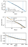 |
Fig. A.1. Density profiles of a simulated halo and the corresponding NFW profile fit. Upper panel: total matter density profile (blue solid line) and the respective NFW profile fit profile (black dashed line). Central panel: reduced shear from simulated particles (orange solid line), and from the analytical projection of the density profile Σconv. presented in Eq. (A.1) and performed in the radial range [60, 3000] kpc, in the blue solid line. The dashed vertical line indicates the minimum radius of the shear fit, and the fit profiles (black lines) are extrapolated down to 10 kpc to enhance the central densities predicted by the two fits. The bottom panel shows the same as the central panel but focuses on the radial range of the fit. The error bars indicate the uncertainty for each radial bin, as defined in Eq. (8). |
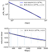 |
Fig. A.2. Density profiles of a mock halo that deviates from NFW and the corresponding NFW profile fit. The mock halo mass, concentration parameter and gNFW log-slopes are chosen to match the ones of the simulated halo presented in Fig. A.1. The upper panel reports the total matter density profile of the mock halo (solid blue line) and the profile from the corresponding NFW profile fit (dashed black line). The bottom panel shows the reduced shear and the profile from the corresponding NFW profile fit (dotted black line). The error bars indicate the uncertainty for each radial bin, as defined in Eq. (8). |
Appendix B: Correlation matrices
In this appendix, we report the correlation coefficient matrices between log-residuals of our mock observables. In Fig. B.2 we show the covariance matrix of non-projected quantities for intermediate redshift objects. In Fig. B.3, we report the correlation matrix as in Fig. B.1 where we present X-ray luminosity, gas mass, and temperature.
We now discuss the differences between scaling relation scatters and covariance values at different overdensities. First of all, we set out to address the fact that when we compute X-ray luminosity within r500c (instead of r200c), we find that the scatter of the scaling relation of the projected quantity is larger than the 3D one.
To investigate this feature, we will focus on the bolometric X-ray luminosity. We report the 3D and projected bolometric X-ray luminosity in Fig. B.4 (top panel), where it is visually clear that the projected X-ray luminosity is (as expected) always larger than the 3D one. One can also notice that the increase in X-ray luminosity depends on the fact that a halo is over-luminous or not: the increase of luminosity growing from the 3D to 2D is larger for under-luminous halos than for over-luminous halos. We prove this point in the bottom panel of Fig. B.4 where we show the ratio between the 2D and 3D luminosity as a function of their residual of the 3D scaling relation (the higher the value of the x axis, the more over-luminous is the object for its mass bin), where we can see a strong anti-correlation: overly luminous objects (for a given mass bin) are not going to be affected much by the fact that their luminosity is computed in 3D or 2D. The possible cause is that an interloper in the LoS will not affect much an overly luminous object.
For completeness, in Fig. B.5 we show the correlation coefficients between the gas mass and stellar mass computed within both r500c and r200c and the concentration. Here we can see a change of sign between M⋆,500c-Mg,500c correlations and M⋆,500c-Mg correlations and a change in the sign between cNFW-Mg correlations and cNFW-Mg,500c correlations.
Finally, in Fig. B.8 we report the scatter of observable properties at fixed mass for both Euclid-like quantities (lensing mass, richness, and projected stellar mass) and possible multi-wavelength properties (integrated Compton-y parameter, X-ray luminosity, and temperature), where we computed the X-ray luminosity and temperature within r500c, as they are typically derived within this overdensity. The upper panel of Fig. B.8 shows the residuals of the log-log linear regression where we see that in terms of 2D scatter, the properties with the lowest scatter are the stellar mass and the temperature. The bottom panel shows the data points used to perform the fit (in black). We used a visually-inspected cut on the halo mass values to ensure that mass values are complete for a given observable value.
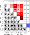 |
Fig. B.1. Correlation coefficients matrix (upper-right triangle) and scatter plot (bottom-left triangle) of power-law log-residuals of Euclid-data (lensing concentration, lensing mass, richness, and stellar mass, respectively) and possible outcomes from multi-wavelength observations (integrated Compton-y parameter, gas mass, X-ray luminosity, and temperature, respectively). Cell colouring goes from blue (negative correlation coefficients) to red (positive correlation coefficients) and is white in the interval [ − 0.35, 0.35] in order to enhance the visibility of the most significant coefficients. |
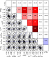 |
Fig. B.3. Same as Fig. B.1 but we show the projected X-ray luminosity, the projected gas mass, and the projected temperature computed within the overdensity of Δc = 500 instead of the respective quantities within Δc = 200. |
Scatter and correlation coefficient matrix between z = 0.24 log-residuals of scaling relations.
Scatter and correlation coefficient matrix between z = 0.9 log-residuals of scaling relations.
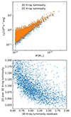 |
Fig. B.4. Comparison between 3D and projected X-ray luminosities. Top panel shows a scatter plot of the two mass-observable relations, while the bottom panel shows their ratio as a function of the 3D X-ray scaling relation residuals. |
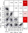 |
Fig. B.5. We report the correlation coefficient between the concentration, gas mass, and stellar mass computed at both r500c and r200c. |
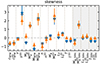 |
Fig. B.7. Same as Fig. 4 but for the data at z = 0.9. We do not report the value for the concentration because in our fit radial range the lensing one does not correlate with the 3D one. |
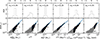 |
Fig. B.8. Halo masses at fixed observable properties. We report the lensing mass, lensing richness, projected stellar mass, projected integrated Compton-y, projected X-ray luminosity, and projected temperature in each column, respectively. The top panel shows residuals of the observable-mass relations and respective scatter of log-residuals σln, and its axes are on the upper part of the plot. The bottom panel shows the scaling relation fit (blue solid line); the data used to perform the fit (black data points) over-plotted on top of the total sample (grey data points) of the mass M as a function of the observable properties. |
All Tables
Scatter and correlation coefficient matrix between z = 0.24 log-residuals of scaling relations.
Scatter and correlation coefficient matrix between z = 0.9 log-residuals of scaling relations.
All Figures
|
Fig. 1. Magneticum mass-observable relation for Euclid-like derived quantities. The left column shows scaling relations, relative fit (solid grey line), and a corridor corresponding to one standard deviation (dashed grey line). The right column shows the residual PDF and scatter of log-residuals σln. We report the following properties: lensing concentration |
| In the text | |
|
Fig. 2. Same as Fig. 1, but for the following multi-wavelength observable properties: Projected integrated Compton-y parameter Y2D (first row), the 3D gas mass Mg, 500c (second row), the projected X-ray luminosity in the soft band (in range [0.5, 2] keV) |
| In the text | |
|
Fig. 3. Scatter of our mass-observable relations, paired with their projected version: concentration, integrated Compton-y parameter, gas mass, NFW mass, richness, stellar mass, X-ray luminosity, and temperature, within a radius of r200c; the grey band reports the gas mass, X-ray luminosity, and temperature within r500c. The left panel reports the fractional scatter of both 3D and 2D quantities. Each dotted vertical line separates the regions that report a given quantity and its 2D version. The right panel reports the contribution of projection effects. Points are coloured by their mass range as in Fig. 1, blue inverted triangles represent the low mass bin, orange up-triangles represent the high mass bin, and grey crosses represent the complete sample. Note: we lack the value of projection effects for LX, 500c (see discussion). Points are ordered according to the value of the second panel. Error bars are computed using the jackknife method. |
| In the text | |
|
Fig. 4. Skewness parameters for our cluster properties. Data, line styles, and colours are as in Fig. 3. Error bars are computed using the jackknife method. |
| In the text | |
|
Fig. 5. Probability density distribution of M2D/M at different mass bins: for halos with M < 2 × 10¹⁴ M⊙ as a blue dotted line, for halos with M > 2 × 10¹⁴ M⊙ as a dashed orange line and for the complete sample as a grey solid line. For each mass bin, the vertical line represents the median values (note: the three lines are very close together). |
| In the text | |
|
Fig. 6. Projected maps along a cylinder of length 23 Mpc, with radius r200c and centred on a random sample of our galaxy clusters, ordered by their M2D/M (over-plotted above each map) values decreasing from left to right. The pixel red, green, and blue channels are used as follows: the red channel maps the gas projected mass, the green channel maps the dark matter projected mass, and the blue channel maps the stellar projected mass. Columns widths are proportional to the cluster radii. |
| In the text | |
|
Fig. 7. Impact of LoS contamination in scaling relations. We show halo properties as a function of halo mass M in the left column, and colour-coded by the fractional amount of mass in a cylinder (M2D/M), and the residuals PDFs in the right column (grey shaded histogram). Rows correspond to richness, the integrated Compton-y parameter, lensing mass, and lensing concentration. We also show the residuals of a subset of halos with low LoS contamination (in particular M2D/M < 1.26, dashed line histogram). Each panel reports the scatter of the residuals σ and the mean μ of the low LoS residuals. |
| In the text | |
|
Fig. 8. Integrated Compton-y parameter vs halo mass, colour-coded by a stellar mass fraction. The top panel shows quantities computed within a sphere of radius r200c, while in the bottom panel, they are computed within a cylinder (of radius r200c and length 23 Mpc as already presented in Sect. 2). We limit the plot in the mass range M ∈ [1, 2]×1014 M⊙. |
| In the text | |
|
Fig. 9. Probability density distribution of the parameters γ (inner slope, upper panel) and β (outer slope, right panel) of Eq. (10) of the successful gNFW profile fits. The central panel shows the scatter plot between the two parameters colour-coded by M. The dotted lines show the NFW parameters γ = 1 and β = 3. |
| In the text | |
|
Fig. 10. Ratio between 2D NFW profile fit parameters and 3D parameters for halos with a successful 3D gNFW profile fit. Upper panel: Ratio between concentrations. Lower panel: Ratio between halo masses. Points are colour-coded by the external log-slope β of the 3D fit of gNFW. |
| In the text | |
|
Fig. 11. Residuals of lensing concentrations with respect to the power-law fit. As in Fig. 7, the dashed line histogram indicates the residuals for objects with low LoS effects (low value of M2D/M). The solid line histogram contains the additional constraints of halos with β and γ parameters close to the ones of an NFW profile (2.8 < β < 3.2 and 0.8 < γ < 1.2). Each histogram label reports the scatter σ of the residuals. |
| In the text | |
|
Fig. 12. Scatter plot of ratio between 2D concentration and 3D concentration against β, namely, the outer slope of Eq. (10), of good 3D gNFW profile fits in a narrow mass range of M ∈ [1, 2]×1014 M⊙. We also report the correlation coefficient. |
| In the text | |
|
Fig. A.1. Density profiles of a simulated halo and the corresponding NFW profile fit. Upper panel: total matter density profile (blue solid line) and the respective NFW profile fit profile (black dashed line). Central panel: reduced shear from simulated particles (orange solid line), and from the analytical projection of the density profile Σconv. presented in Eq. (A.1) and performed in the radial range [60, 3000] kpc, in the blue solid line. The dashed vertical line indicates the minimum radius of the shear fit, and the fit profiles (black lines) are extrapolated down to 10 kpc to enhance the central densities predicted by the two fits. The bottom panel shows the same as the central panel but focuses on the radial range of the fit. The error bars indicate the uncertainty for each radial bin, as defined in Eq. (8). |
| In the text | |
|
Fig. A.2. Density profiles of a mock halo that deviates from NFW and the corresponding NFW profile fit. The mock halo mass, concentration parameter and gNFW log-slopes are chosen to match the ones of the simulated halo presented in Fig. A.1. The upper panel reports the total matter density profile of the mock halo (solid blue line) and the profile from the corresponding NFW profile fit (dashed black line). The bottom panel shows the reduced shear and the profile from the corresponding NFW profile fit (dotted black line). The error bars indicate the uncertainty for each radial bin, as defined in Eq. (8). |
| In the text | |
|
Fig. B.1. Correlation coefficients matrix (upper-right triangle) and scatter plot (bottom-left triangle) of power-law log-residuals of Euclid-data (lensing concentration, lensing mass, richness, and stellar mass, respectively) and possible outcomes from multi-wavelength observations (integrated Compton-y parameter, gas mass, X-ray luminosity, and temperature, respectively). Cell colouring goes from blue (negative correlation coefficients) to red (positive correlation coefficients) and is white in the interval [ − 0.35, 0.35] in order to enhance the visibility of the most significant coefficients. |
| In the text | |
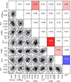 |
Fig. B.2. Same as Fig. B.1 but here we show the quantities computed in the 3D space. |
| In the text | |
|
Fig. B.3. Same as Fig. B.1 but we show the projected X-ray luminosity, the projected gas mass, and the projected temperature computed within the overdensity of Δc = 500 instead of the respective quantities within Δc = 200. |
| In the text | |
|
Fig. B.4. Comparison between 3D and projected X-ray luminosities. Top panel shows a scatter plot of the two mass-observable relations, while the bottom panel shows their ratio as a function of the 3D X-ray scaling relation residuals. |
| In the text | |
|
Fig. B.5. We report the correlation coefficient between the concentration, gas mass, and stellar mass computed at both r500c and r200c. |
| In the text | |
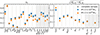 |
Fig. B.6. Same as Fig. 3 but for the data at z = 0.9. |
| In the text | |
|
Fig. B.7. Same as Fig. 4 but for the data at z = 0.9. We do not report the value for the concentration because in our fit radial range the lensing one does not correlate with the 3D one. |
| In the text | |
|
Fig. B.8. Halo masses at fixed observable properties. We report the lensing mass, lensing richness, projected stellar mass, projected integrated Compton-y, projected X-ray luminosity, and projected temperature in each column, respectively. The top panel shows residuals of the observable-mass relations and respective scatter of log-residuals σln, and its axes are on the upper part of the plot. The bottom panel shows the scaling relation fit (blue solid line); the data used to perform the fit (black data points) over-plotted on top of the total sample (grey data points) of the mass M as a function of the observable properties. |
| In the text | |
Current usage metrics show cumulative count of Article Views (full-text article views including HTML views, PDF and ePub downloads, according to the available data) and Abstracts Views on Vision4Press platform.
Data correspond to usage on the plateform after 2015. The current usage metrics is available 48-96 hours after online publication and is updated daily on week days.
Initial download of the metrics may take a while.