| Issue |
A&A
Volume 695, March 2025
|
|
|---|---|---|
| Article Number | A85 | |
| Number of page(s) | 13 | |
| Section | Astrophysical processes | |
| DOI | https://doi.org/10.1051/0004-6361/202451211 | |
| Published online | 11 March 2025 | |
Spectral properties of the neutron star low-mass X-ray binaries 4U 1636–53, XTE J1739–285, and MAXI J1816–195
1
Department of Physics, Xiangtan University, Xiangtan, Hunan 411105, China
2
Key Laboratory of Stars and Interstellar Medium, Xiangtan University, Xiangtan, Hunan 411105, China
3
Yunnan Observatories, Chinese Academy of Sciences (CAS), Kunming 650216, PR China
4
Key Laboratory for the Structure and Evolution of Celestial Objects, CAS, Kunming 650216, PR China
5
Instituto Argentino de Radioastronomía (CCT La Plata, CONICET; CICPBA; UNLP), C.C.5, (1894) Villa Elisa, Argentina
⋆ Corresponding author; This email address is being protected from spambots. You need JavaScript enabled to view it.
Received:
21
June
2024
Accepted:
15
January
2025
Abstract
We investigated simultaneous NICER plus NuSTAR observations of the three neutron star low-mass X-ray binaries 4U 1636–53, XTE J1739–285, and MAXI J1816–195 using the latest reflection models. The seed photons in our models that are fed into the corona originated from either the neutron star (NS) or the accretion disk. We found that for the sources in the hard spectral state, more than ∼50% of the NS photons enter the corona when the NS provides seed photons, while only ∼3–5% of the disk photons enter the corona when the seed photons come from the disk. This finding, together with the derived small height of the corona, favors a lamp-post geometry or a boundary layer scenario in which the corona is close to the central NS. Additionally, we found that the source of the seed photons has a strong influence on the significance of the NS radiation, especially for the soft spectral state. This result may help us to explain why the NS radiation in MAXI J1816–195 was weak in previous work. More importantly, for the first time, we explored the properties of the corona in the NS systems with the compactness (l − θ) diagram. We found that coronae in NS systems all lie on the left side of the pair-production forbidden region, away from the predicted pair-production lines. This finding indicates that either the corona in these NS systems is not pair dominated, possibly due to the additional cooling from NS photons, or the corona is composed of both thermal and nonthermal electrons.
Key words: accretion / accretion disks / binaries: spectroscopic / stars: neutron
© The Authors 2025
 Open Access article, published by EDP Sciences, under the terms of the Creative Commons Attribution License (https://creativecommons.org/licenses/by/4.0), which permits unrestricted use, distribution, and reproduction in any medium, provided the original work is properly cited.
This article is published in open access under the Subscribe to Open model. This email address is being protected from spambots. You need JavaScript enabled to view it. to support open access publication.
1. Introduction
X-ray binaries are systems that are composed of a compact object and a main-sequence or post-main-sequence companion star. When the mass of the companion star is lower than 1 M⊙, the system is classified as a low-mass X-ray binary (LMXB), which can be further divided into a black hole (BH) LMXB or a neutron star (NS) LMXB, according to the nature of the central compact object. In an LMXB, the compact object accretes matter from the companion via Roche-lobe overflow (Tauris & van den Heuvel 2006), and a vast amount of the gravitational potential energy is released in X-rays.
The two types of LMXBs are different. The most obvious difference is the physical surface in an NS LMXB, which can lead to significant observation features such as thermonuclear bursts or millihertz (mHz) quasi-periodic oscillations (QPOs) because of the nuclear burning of the accreted material that accumulated on the surface (e.g., Lewin et al. 1993; Revnivtsev et al. 2001; Strohmayer & Bildsten 2006; Heger et al. 2007; Lyu et al. 2015), a different behavior of the spectral evolution (Done & Gierliński 2003), or pulsation caused by the residual magnetic field (Done et al. 2007). An NS system also has a so-called boundary or spreading layer (Syunyaev & Shakura 1986; Inogamov & Sunyaev 1999) between the innermost part of the accretion disk and the surface of the neutron star. Infalling matter decelerates from the Keplerian velocity at the inner accretion flow to the surface rotation velocity of the NS in this region, and its kinetic energy is deposited.
The radiation scenario in an NS LMXB is more complicated than in a BH LMXB. LMXBs usually have multicolor thermal emission from the accretion disk and nonthermal power-law radiation from a corona that is composed of high-energy plasma. In addition, the power-law photons could illuminate the disk and hence generate a reflection component. Additional thermal radiation from the NS surface exists in an NS system, however, and this thermal emission could also illuminate and then be reflected off the accretion disk. Furthermore, the thermal photons from the NS surface could enter the corona and be upscattered as power-law photons.
Observationally, the spectral properties of the NS LMXBs have been widely investigated, but the role of the NS radiation is still unclear. On the one hand, the influence of the NS illumination on the disk is poorly understood. Only the scenario in which the disk is illuminated and ionized by the corona alone has been investigate in most works, while studies focusing on the NS illumination are rare (e.g., Cackett et al. 2010; Wilkins 2018; Ludlam et al. 2020, 2022; García et al. 2022; Lyu et al. 2023). On the other hand, due to possible degeneracy problems (e.g., Sanna et al. 2013; Lyu et al. 2014), the scenario in which the seed photons come from the NS surface for the Compton scattering is currently not fully explored.
In order to obtain more insight into the influence of the neutron star radiation, we investigated three NS LMXBs that were simultaneously observed by the Neutron Star Interior Composition Explorer (NICER) detector and the Nuclear Spectroscopic Telescope Array (NuSTAR) telescope. We briefly introduce these three sources below.
The source 4U 1636–53 harbors a millisecond pulsar with a spin frequency of 581 Hz (Zhang et al. 1997; Strohmayer & Markwardt 2002). Its orbital period is 3.8 h (van Paradijs et al. 1990) at a distance of 6.0 ± 0.5 kpc (Galloway et al. 2006). This source shows various observational features such as thermonuclear bursts, superbursts, mHz QPOs, kilohertz (kHz) QPOs, and time lags. In addition, 4U 1636–53 shows the evolution of all the spectra states (Belloni et al. 2007; Altamirano et al. 2008), with a regular state transition cycle of ∼40 days (Shih et al. 2005; Belloni et al. 2007).
For the source XTE J1739–285, Galloway et al. (2008) derived a distance shorter than 7.3 kpc based on the peak flux of photospheric radius-expansion (PRE) bursts. Bailer-Jones et al. (2018) estimated a distance of 4 kpc with parallaxes published in the Gaia data. The Fe Kα line and a Compton hump were detected in the spectrum of this source (Mondal et al. 2022). Kaaret et al. (2007) reported a 1122 Hz burst oscillation in XTE J1739–285, indicating that it may be the only discovered neutron star that rotates within a submillisecond period. Later studies did not detect this special burst oscillation, however (Galloway et al. 2008; Bilous & Watts 2019; Bult et al. 2021). Bult et al. (2021) found that a 386.5 Hz oscillation was the more prominent signal and hypothesized that the rotation period of XTE J1739–285 might not be a submillisecond period.
The source MAXI J1816–195 is a new accreting millisecond X-ray pulsar (AMXP) discovered by the Monitor of All-sky X-ray Image (MAXI) Gas Slit Camera (GSC) on June 7, 2022 (Negoro et al. 2022). Its circular orbital period is ∼4.8 hours (Bult et al. 2022a), and the spin frequency of MAXI J1816–195 is 528 Hz (Bult et al. 2022b). Chen et al. (2022) derived the upper limit of its distance to be 6.3 kpc from the peak flux of the brightest burst detected by the Hard X-ray Modulation Telescope (Insight-HXMT) from June 8 to 30, 2022. Bult et al. (2022a) obtained an upper limit of 8.6 kpc from the peak flux of bursts with NICER. Moreover, Li et al. (2023a) reported the detection of X-ray pulsations in this source up to ∼95 keV.
2. Observations and data reduction
We analyzed simultaneous NICER plus NuSTAR observations of 4U 1636–53, XTE J1739–285, and MAXI J1816–195. These observations (Table 1) were made from April 2019 to June 2022, and the total exposure time was ∼26.4 ks and ∼153 ks for the NICER and the NuSTAR observations, respectively. We used HEASOFT version 6.30.1 to reduce the data from the two satellites.
NICER/NuSTAR observations of the three NS LMXBs.
2.1. NICER observations
NICER is located on the International Space Station (ISS). The X-ray Timing Instrument (XTI) operates in the soft X-ray range of 0.2–12 keV (Gendreau et al. 2016). The energy resolution is ∼85 eV at 1 keV and ∼137 eV at 6 keV1. We performed the standard data reduction using the NICER Data Analysis Software and the latest calibration files, version 20240206. The clean XTI events were extracted using the command nicerl2, and we applied the standard calibration. Time intervals containing X-ray bursts were removed by the tool xselect. We obtained the background by running the tool nibackgen3C50 (Remillard et al. 2022), and we used the commands nicerrmf and nicerarf to produce the response matrix files (RMFs) and the ancillary response files (ARFs). Finally, we applied the command grppha to group the spectra to ensure a minimum of 100 counts per bin.
2.2. NuSTAR observations
NuSTAR has two independent detectors, FPMA and FPMB, which operate in a broad energy range of 3–79 keV, with a spectral energy resolution of 400 eV (FWHM) at 10 keV (Harrison et al. 2013). The data from the two detectors were calibrated and screened to obtain clean events with the pipeline tool nupipeline using the latest calibration files, version 20240916. We applied the script nuproducts to extract the source and background spectra using a circular region of radius 150 arcsec. The response and ancillary response files were produced simultaneously with this script. The spectra were rebinned with the default option grpmincounts = 100 in nuproducts.
As shown in Figure 1, there are 4 and 15 bursts in the NICER and the NuSTAR observation of 4U 1636–53. For MAXI J1816–195, there are 2 bursts in the NICER data and 4 bursts in the NuSTAR data. The number of bursts in the NICER and the NuSTAR observation of XTE J1739–285 is 0 and 2, respectively.
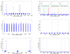 |
Fig. 1. NICER (left panel) and NuSTAR/FPMA (right panel) light curve of 4U 1636–53 (top), XTE J1739–285 (middle), and MAXI J1816–195 (bottom). We extracted NICER light curves in 0.5–10 keV at a time resolution of 1 second, and we derived the NuSTAR light curves in 3–79 keV using a time bin of 5 seconds. |
In order to study the spectral state of the sources, we further generated the hardness-intensity diagram (HID) (Figure 2) using the NICER observations. We first extracted light curves in the 0.5–4 keV, 4–10 keV, and 0.5–10 keV bands every 64 seconds. We then calculated the hardness as the count-rate ratio between 4–10 keV and 0.5–4 keV, and we defined the intensity as the count rate in 0.5–10 keV. We found that the spectra of 4U 1636–53 and XTE J1739–285 were in the hard spectral state, and MAXI J1816–195 was in a much softer state.
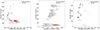 |
Fig. 2. Hardness-intensity diagram of NICER observations of 4U 1636–53 (left), XTE J1739–285 (middle), and MAXI J1816–195 (right). The hardness ratio is defined as the count ratio of the 4–10 and 0.5–4 keV, and the intensity is defined as the counts in 0.5–10 keV. Each datapoint in the plots corresponds to a 64-second NICER data segment, with the NICER observations analyzed in this work shown in red and other NICER observations marked in gray. |
3. Spectral analysis
We used XSPEC version 12.12.1 to simultaneously fit the NICER and the NuSTAR spectra. We first selected an energy range of 1.0–70 keV, with the NICER and the NuSTAR data covering 1.0–10.0 keV (e.g., Mondal et al. 2022) and 3.0–70 keV (e.g., Mondal et al. 2019; Kargaltsev et al. 2023; Dias et al. 2024), respectively. However, we found that residuals remained at the low energies of the NuSTAR spectra, similar to the residuals caused by a possible instrumental difference reported by Madsen et al. (2020). We thus ignored the NuSTAR data below 4 keV. For XTE J1739–285, we only used the energy up to 60 keV as the spectra became background dominated above this. During the fits, we selected the model tbabs to describe the interstellar absorption along the line of sight, using the solar abundance of Wilms et al. (2000) and the photon-ionization cross-section table of Verner et al. (1996). A constant component was added to describe the possible cross-calibration between different instruments.
We first tried a simple model bbodyrad + diskbb + cutoffpl to estimate the spectra shape. The bbodyrad component fits the thermal radiation from the neutron star surface, and the diskbb component (Mitsuda et al. 1984; Makishima et al. 1986) describes multicolor blackbody emission from the accretion disk. We also included a gauss component to fit the possible iron emission line in 6.4–6.97 keV. We found that the spectra were only poorly described, possibly due to the lack of a reflection continuum in the model. We then replaced the cutoffpl component with the physical model thcomp (Zdziarski et al. 2020). The thcomp is a convolution thermal-Comptonization model that is thought to represent the thermal Comptonization more accurately than the simple cutoffpl component because it takes the electron temperature kTe and the cover fraction parameter fcov into account. We selected either the bbodyrad component or the diskbb component as the source of the seed photons for the thcomp component. We also extended the energy by the command “energies 0.01 1000.0 1000 log” for the application of the thcomp.
We also replaced the gauss component with the more physical reflection model family relxill (García et al. 2014; Dauser et al. 2016). Based on the xillver reflection code (García & Kallman 2010; García et al. 2013) and the relline ray-tracing model (Dauser et al. 2010, 2013), the relxill models are able to calculate the reflection off the accretion disk at each emission angle. We applied the model relxillCp and the model relxilllpCp to fit the spectra of the three sources. The relxillCp model uses a nthcomp illuminating spectrum, and the relxilllpCp model assumes a lamp-post geometry where the corona is a point source located at a height above the central compact object. The parameters in the model relxillCp are the spin parameter, a, the inclination angle, incl, the inner and outer radii of the disk Rin and Rout, the emissivity index of the inner and outer disk, qin and qout, the breaking radius, Rbr, where the emissivity changes; the ionization parameter, ξ, the power-law index of primary source, Γ, the electron temperature, kTe, the disk density, log(N), the iron abundance, AFe, the reflection fraction, frefl, the redshift, z, and the normalization. For the relxilllpCp model, most of the parameters are the same as in relxillCp, but we replaced the emissivity index with two new parameters, the height of the corona, h, and the velocity of the primary source, β.
In the fits, we fixed the frefl parameter at –1 so that only the reflection component was returned. The emissivities were fixed at the typical value of 3, and the broken radius Rbr was set to be equal to the outer radius Rout, which was fixed at 1000 Rg. The redshift was set to zero, and the disk density, log(N), was fixed at 20. The spin parameter a was calculated according to the formula a = 0.47/Pms (Braje et al. 2000), where Pms is the spin period of the neutron star in milliseconds. The derived spins for 4U 1636–53, XTE J1739–285, and MAXI J1816–195 are 0.27, 0.18, and 0.25, calculated from a spin frequency of 581 Hz (Zhang et al. 1997; Strohmayer & Markwardt 2002), 386 Hz (Bult et al. 2021), and 528 Hz (Bult et al. 2022b), respectively. The primary source velocity, β, was set to zero since it is only poorly constrained in the fits.
For the MAXI J1816–195 data reported in the soft state (Mandal et al. 2023), we further applied another reflection model diskbb + compTT + relxillns to explore its properties when the disk is illuminated by the NS surface instead of the corona. The compTT model describes the thermal Comptonization component from the corona (Titarchuk 1994), and the parameters are the seed photon temperature, T0, the plasma temperature, kTe, the plasma optical depth, τ, the geometry switch, approx, and the normalization. We set the approx to 2 to select the sphere geometry and let T0 free to vary in the fit. The model relxillns (García et al. 2022) was developed to explain the reflection from the accretion disk illuminated by a blackbody component. In the relxillns model, the parameters are the same as in the relxillCp model, except that there is no kTe and Γ, but instead, a new parameter kTBB. The parameter log(ξ) was fixed to its maximum allowed value 19, and the emissivity index was set to its typical value of 3. In the fits of MAXI J1816–195, we found an edge-like residual near ∼1.8 keV, similar to the one reported by Li et al. (2023b). This residual was proposed to be caused by the NICER calibration systematics, and we therefore applied an additional edge model to fit it.
To summarize, we used the reflection models with different illumination sources for the spectra of the three sources (Table 2). For the spectra of MAXI J1816–195 reported in the soft state, we applied an additional model in which the disk is illuminated by the NS surface.
Reflection models applied to the spectra of the three NS LXMBs.
4. Results
In Table 3 we show the best-fitting results for 4U 1636–53 with the reflection model relxillCp and relxilllpCp. We found that the temperature of the neutron star is in the range of ∼1.3–1.8 keV, and the temperature of the accretion disk is ∼0.16–0.17 keV regardless of the type of seed thermal photons. The power-law index, Γ, is around 1.5–1.7, the derived inner radius of the disk exceeds ∼6.6 Rg, and with the normalization of the diskbb component is larger than 7.5 × 10⁴ in the all fits. These results are consistent with previous reports that the source was in the hard spectral state (Mondal et al. 2021). The ionization parameter log(ξ) is ∼3.6–4.0, indicating that the disk is highly ionized. The height of the corona in the lamp-post geometry is very low, ∼2.3–2.5 Rg. Interestingly, the cover fraction parameters (fcov) in the case of NS seed photons are ∼50–80%, while they are ∼5% when the seed photons come from the disk.
Best-fitting results for the fits to the X-ray spectra of 4U 1636–53 with the reflection model M1–M4.
In Table 4 we list the fitting results for XTE J1739–285. The derived disk temperature is ∼0.14–0.15 keV, and Ndbb is higher than 5.0 × 10⁴. The temperature of the blackbody thermal emission lies in the range of ∼0.9 keV to ∼1.5 keV. The derived corona height is  Rg and
  Rg in the NS seed photon case and the disk seed photon case, respectively. The cover fraction is larger than ∼80% in the NS seed photon case and smaller than ∼3% in the disk seed photon case. We show the corresponding spectra, individual components, and residuals of the fits for 4U 1636–53 and XTE J1739–285 in Figures 3 and 4.
Best-fitting results for the fits to the X-ray spectra of XTE J1739–285 with the reflection model M1–M4.
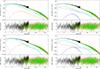 |
Fig. 3. Best-fitting results with different reflection models (M1 and M2 from left to right at the top; M3 and M4 at the bottom) for NICER/NuSTAR observations of 4U 1636–53. We show the fitted spectra and the individual model components (main panel), and the residuals in terms of sigmas (subpanel) in the plots. The components diskbb, blackbody, (thcomp × diskbb) or (thcomp × bb), and relxillCp or relxilllpCp are plotted with the dotted purple line, the dot-dashed deep blue line, the dashed orange line, and the solid light blue line, respectively. |
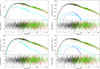 |
Fig. 4. Best-fitting results with different reflection models (M1 and M2 from left to right at the top; M3 and M4 at the bottom) for NICER/NuSTAR observations of XTE J1739–285. We show the fitted spectra and the individual model components (main panel), and the residuals in terms of sigmas (subpanel) in the plots. The components diskbb, blackbody, (thcomp × diskbb) or (thcomp × bb), and relxillCp or relxilllpCp are plotted with the dotted purple line, the dot-dashed deep blue line, the dashed orange line, and the solid light blue line, respectively. |
In Table 5 we show the fitting results of MAXI J1816–195 with the model relxillCp and relxilllpCp. The accretion disk is relative hot, ∼0.5–0.6 keV, and the normalization of the diskbb component is lower than ∼2100. The blackbody temperature is ∼1–1.1 keV and ∼1.3–1.4 keV in the case of NS seed photon and disk seed photon, respectively. The photon index Γ is ∼2, and the electron temperature kTe is ∼13–15 keV. The derived height of the corona is ∼3 Rg, and the disk is moderately ionized, with an ionization parameter log(ξ) ∼ 2.2. The derived cover fraction parameter is ∼0.8 in the NS seed photon case, and it is relative low, ∼0.3 in the disk seed photon case. Interestingly, in both models, we found that the normalization of the blackbody component changes significantly from ∼5 in the disk seed photon case to be higher than ∼62 in the NS seed photon case, indicating that the source of the seed photons probably greatly influences the neutron star radiation. The corresponding spectra, individual components, and residuals of the fits are shown in Figure 5.
Best-fitting results for the fits to the X-ray spectra of MAXI J1816–195 with reflection model M1–M4.
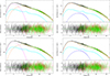 |
Fig. 5. Best-fitting results with different reflection models (M1 and M2 from left to right at the top; M3 and M4 at the bottom) for NICER/NuSTAR observation of MAXI J1816–195. We show the fitted spectra and the individual model components (main panel), and the residuals in terms of sigmas (subpanel) in the plots. The components diskbb, blackbody, (thcomp × diskbb) or (thcomp × bb), and relxillCp or relxilllpCp are plotted with the dotted purple line, the dot-dashed deep blue line, the dashed orange line, and the solid light blue line, respectively. |
In Table 6 we show the results of the fit of model M5. The fitted temperature of the bbodyrad and diskbb components is ∼2.32 keV and ∼0.60 keV, respectively. The temperature of the seed photons for the corona is 0.98 ± 0.04 keV, which is in between the one of the bbodyrad and the diskbb, suggesting that the seed photons are likely a mixture of the two components. The electron temperature kTe in the corona is  keV, with the optical depth being
  . The ionization parameter of the disk is similar to that in relxillCp and relxilllpCp, log(ξ) ∼ 2. The inner radius of the disk is smaller than ∼9.25 Rg, with the reflection fraction parameter in relxillns being ∼21. The corresponding spectra, individual components, and residuals of the fits are presented in Figure 6.
Best-fitting results for the fit to the X-ray spectra of MAXI J1816–195 with reflection model M5.
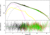 |
Fig. 6. Best-fitting results with the reflection model M5 for NICER/NuSTAR observation of MAXI J1816–195. We show the fitted spectra and the individual model components (main panel), and the residuals in terms of sigmas (subpanel) in the plots. The components diskbb, compTT, and relxillns are plotted with the dotted purple line, the dashed gray line, and the solid yellow line, respectively. |
5. Discussion
We investigated the three neutron star low-mass X-ray binaries with simultaneous NICER plus NuSTAR observations. We found that in the hard spectral state, when the seed photons come from the NS, more than ∼50% of the NS photons go into the corona. When the seed photons come from the accretion disk, however, only ∼3–5% of the disk photons move into the corona. Furthermore, the height of the corona is very small, ∼2–3 Rg from the central compact object. More importantly, we found that the seed photon type significantly affects the inferred neutron star radiation.
5.1. Boundary layer and magnetic field in 4U 1636–53 and XTE J1739–285
The derived inner disk radii of 4U 1636–53 and XTE J1739–285 are larger than the typical NS radius, suggesting that the disk may be truncated by a certain mechanism. We thus first estimated the radius of the boundary layer from the mass-accretion rate based on the formula below (Popham & Sunyaev 2001),
 (1)
(1)
with the mass-accretion rate, ṁ, calculated using the equation (Galloway et al. 2008; Giridharan et al. 2024)
 (2)
(2)
where Fbol is the total bolometric flux in units of 10−9 erg cm−2 s−1, z is the surface redshift, and D10 is the distance of the source in units of 10 kpc. We used a distance of 6 kpc (Galloway et al. 2006) and 4 kpc (Bailer-Jones et al. 2018) for 4U 1636–53 and XTE J1739–285, respectively. We took Fbol as the total unabsorbed flux in 0.1–100 keV in the fits, and calculated  (Thomas et al. 2023), where MNS = 1.4 M⊙ and RNS = 10 km. The derived maximum boundary layer radius is ∼6–7 Rg and ∼5 Rg for 4U 1636–53 and XTE J1739–285, respectively.
Assuming that the accretion disk is truncated by a magnetic field for 4U 1636–53 and XTE J1739–285 in hard state, we placed an upper limit on the strength of the field using the following equation (Cackett et al. 2009),  , where μ is the magnetic dipole moment, kA is the coefficient that depends on the conversion from spherical to disk accretion, x is given from Rin = xGM/c2 (Cackett et al. 2009), fang is the anisotropy correction factor, and η is the accretion efficiency.
We then calculated the magnetic field of the sources based on B = μ/R3 (Long et al. 2005), where R is the radius of the neutron star. During the calculation, we set kA = 1, fang = 1, η = 0.1, M = 1.4 M⊙, R = 10 km, and Fbol = F0.1 − 100 keV. We took Rin and Fbol from the fits with model M1 and obtained the polar magnetic field of 4U 1636–53 and XTE J1739–285 as B ≤ 1.9 × 10⁹ G and B ≤ 2.8 × 10⁹ G, respectively.
The calculated upper limit of the magnetic field in XTE J1739–285 slightly exceeds that (B ≤ 6.2 × 10⁸ G) reported by Mondal et al. (2022). For 4U 1636–53, Strohmayer (1999) proposed that there likely is a stronger magnetic field in this source than others because 4U 1636–53 alone shows significant pulsations at the subharmonic of the strongest oscillation frequency. Mondal et al. (2021) estimated a magnetic field strength of 4U 1636–53 at the poles of B < 2.0 × 10⁹ G, which is close to the value we derived here. The magnetic field measured in Mondal et al. (2021) and in this work lie in the typical range of 108 G to 109 G (e.g., Mukherjee et al. 2015; Ludlam et al. 2016, 2017; Mondal et al. 2019). This shows no clear indication that 4U 1636–53 has a stronger magnetic field than others.
5.2. Corona geometry
In the current stage, the physical and geometrical properties of the corona are still unclear. Three typical types of the corona model were proposed: (1) A static corona with different geometries (e.g., slab; Haardt et al. 1994), (2) the base of a jet (Markoff et al. 2001, 2005), and (3) a radiatively inefficient accretion flow (RIAF; Ferreira et al. 2006; Narayan & McClintock 2008). It was also proposed that the boundary layer likely plays the role of the corona in neutron star systems (e.g., Popham & Sunyaev 2001; D’Aì et al. 2010; Saavedra et al. 2023).
The cover fraction of the seed photons is important for understanding the position and geometry of the corona. The fraction derived in this work favors corona models in which the corona is close to the central compact object in the hard state: In this case, many photons from the NS might reach the nearby corona, and thus, the corresponding cover fraction is high (higher than ∼ 50% in our results). The disk is far from the neutron star in the hard state, however, so that the fraction of the disk photons that enter the corona is low (only ∼3–5% in our fits). This scenario is also supported by the derived small height of the corona in our fits.
These results support both the lamp-post geometry and the boundary layer scenario. In the well-known lamp-post case, the corona could be the base of a jet, or a moving hot plasma situated above the spin axis of the central compact object. When the height of the corona is small, a large fraction of the thermal photons from NS surface might reach the corona and be Compton scattered, consistent with the large cover fraction we derived. In the boundary layer, the infalling matter decelerates from its orbital velocity in the accretion disk to the rotation velocity of the neutron star surface (Syunyaev & Shakura 1986; Inogamov & Sunyaev 1999). Popham & Sunyaev (2001) found that the main part of the boundary layer is hot (≥108 K) and is vertically and radially extended. For LMXBs in the low-hard state, Comptonization in the hot boundary layer is able to generate a power-law spectrum with a cutoff energy of ∼20–30 keV. Observationally, Wang et al. (2017) derived a small height of the corona (∼2–3 Rg) in 4U 1636–53 with NuSTAR observations. They therefore proposed that the hard X-rays likely come from the boundary layer. Similarly, Thompson et al. (2005) applied two Comptonization components for the spectroscopy of the GS 1826–238, one of which was proposed to come from or from the vicinity of the boundary layer. Interestingly, the derived maximum boundary layer radius (∼5–7 Rg) in this work is close to the height of the corona (∼3 Rg). The boundary layer might therefore play the role of the corona in the two hard observations in this work.
One way to distinguish a moving corona or base of a jet from a boundary layer is to determine whether the corona has a high velocity. For a moving corona or jet base, they should have mildly relativistic velocities (Beloborodov 1999; King et al. 2017), while in the case of a boundary layer, Popham & Sunyaev (2001) showed that the radial velocity is well below the sound speed in their calculations. We were unable to constrain the velocity of the corona in the component relxilllpCp. Observations with long enough exposure times are required in the future to separate the lamp-post geometry and the boundary layer for the NS systems.
5.3. Corona compactness
We also studied the physics of the corona for NS systems with the so-called compactness (ℓ–θ) diagram (Figure 7). The ℓ–θ diagram was proved to be a useful tool for understanding the physics inside the corona (e.g., Fabian et al. 2015, 2017; Zdziarski et al. 2021; Kang & Wang 2022; Bertola et al. 2022; Kamraj et al. 2022; Tortosa et al. 2022; Hinkle & Mushotzky 2021; Kang et al. 2021; Reeves et al. 2021). In the ℓ–θ diagram, the dimensionless compactness parameter ℓ (Guilbert et al. 1983) represents the ratio of the corona luminosity to its size, and θ is proportional to the electron temperature. Physically, when power is fed into the corona, the electron temperature increases, and thus, the scattering of the soft seed photons generates more energetic power-law photons. As the power-law spectrum extends to a Wien tail above ∼2 mec2, the photon-photon collisions could create electron-positron pairs. In this case, a new injection of energy into the corona could not lead to the increase in the corona temperature, but instead results in an increase in the number of pairs. This means that there should be a pair-production limit in the ℓ–θ diagram if the corona is pair dominated.
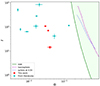 |
Fig. 7. Compactness–temperature (ℓ–θ) diagram for the NS LMXBs. We use different symbols to mark the samples in this work and in the literature (Table 7). |
Fabian et al. (2015) showed that the corona in AGNs is hot and radiatively compact, lying close to the pair run-away line in the ℓ–θ diagram. This finding suggests that the temperature of the corona in these AGNs might be regulated by pair production and annihilation. Later, Fabian et al. (2017) proposed that the corona lying well below the pair limit might also be pair dominated if the corona contains nonthermal electrons, which is able to decrease the pair-production threshold temperature.
Interestingly, a corona lying beyond the predicted pair runaway line was also reported in AGNs and black hole binary (BHB) systems. Kang & Wang (2022) recently found that a considerable fraction of AGNs lie beyond the boundaries of the forbidden areas due to runaway pair production. They proposed that the corona likely is more extended than 10 Rg in these systems. Furthermore, for the accreting black hole binary XTE J1752–223 in the hard state, Zdziarski et al. (2021) found that the compactness is much higher than the maximum allowed by pair equilibrium. The reason for this discrepancy is still unclear.
The compactness of the corona in neutron star binaries is studied far more rarely than those in black hole systems. For the first time, we show the ℓ–θ diagram for nine NS systems (including samples taken from literature as listed in Table 7) in Figure 7. The compactness is calculated as  (Fabian et al. 2015), where mp and me is the mass of proton and electron, and R and L is the corona radius and luminosity. In the calculation, corona size R is assumed to be 10 Rg (Fabian et al. 2015). The parameter θ is defined as θ = kTe/mec2, where kTe is estimated as kTe = Ecut/2 when the kTe is no available in the literature. For the three sources analyzed in this work, the corona luminosity L was derived from the corona flux in 0.1–100 keV, and the kTe was taken directly from the fits with the relxilllpCp model. In the figure, we also overplot the pair runaway lines for the three geometries (Stern et al. 1995) and show the runaway pair-production forbidden region (green area) for the slab geometry. Apparently, all the NS systems lie to the left side of the pair-production forbidden region, away from the slab pair line. This result suggests that the corona in these NS systems is likely not composed of electron-positron pairs, which could be explained by the additional cooling by the thermal seed photons from the neutron star surface. With this cooling process, the temperature of the electrons in the corona is relative low, and consequently, the power-law photons generated by Compton scattering would not be energetic enough to create electron-positron pairs in the following photon-photon collisions. The corona in the NS systems would therefore not be pair dominated. If the above scenario is true, then it again constitutes evidence that the seed photons from the NS surface are crucial for the physics of the neutron star systems.
However, we cannot rule out the possibility that the corona is a hybrid plasma that contains both thermal and nonthermal particles. In this case, a corona with cooler temperatures may still be regulated by the pair-production process since its threshold temperature is decreased by the nonthermal electrons, in the same way as described by Fabian et al. (2017).
5.4. Spectral properties of MAXI J1816–195
Li et al. (2023b) studied the NICER plus the NuSTAR observation of MAXI J1816–195 and found that the thermal radiation from the neutron star surface is not significant, with a blackbody temperature ∼2.05 keV and a normalization Nbb < 2. This scenario is consistent with the weak blackbody component in our fitting result when the seed photons come from the accretion disk (M2 and M4 in Table 5). However, the blackbody component is not weak when the seed photons are supplied by the neutron star surface (M1 and M3 in Table 5), indicating that the source of the seed photons could greatly influence the significance of the neutron star radiation. This is natural because in the latter case the neutron star needs to provide additional photons for the Compton scattering, so that a stronger blackbody component is required. Furthermore, the seed photon type also influences the derived radius of the emitting region on the NS surface, as the radius is directly linked to the parameter Nbb. Therefore, determining the source of the seed photons is a prerequisite for accurately estimating the emitting region on the neutron star surface.
Mandal et al. (2023) applied the model diskbb + nthcomp to the preburst spectra of MAXI J1816–195 from the same NICER and NuSTAR observation as we used. They found that the corresponding electron temperature was relatively low, ∼11 keV, and thus, they deduced that the source is in the soft spectra state. This result is interesting because most of the AMXPs are typically observed in hard spectral states, with SAX J1748.9–2021 (Pintore et al. 2016) and SAX J1808.4–3658 (Di Salvo et al. 2019) as perhaps the only two exceptions reported in the soft state. For AMXPs in the hard state, the electron temperature is generally high at some dozen keV (e.g., Gierliński & Poutanen 2005; Sanna et al. 2017, 2018; Rai & Paul 2019; Di Salvo & Sanna 2022), and the NS thermal emission is usually found with relatively low temperatures, that is, below 1 keV (e.g., Sanna et al. 2017, 2022; Rai & Paul 2019; Marino et al. 2022). We applied the latest reflection models and obtained a relative high blackbody temperature (∼1–1.4 keV) plus a low electron temperature ∼13–15 keV. More importantly, the derived inner radius of the disk from the reflection component is small, ∼RISCO, consistent with the previously measured radius, Rin = 1.04 − 1.23 RISCO by Li et al. (2023b). Thus, the relative high blackbody temperature, the low electron temperature, and the very small inner radius together suggest that MAXI J1816–195 in this observation is likely not in the hard state and is instead in the soft state or in a transitional state.
6. Conclusion
Benefiting by the wide energy range covered by the NICER detector and the NuSTAR satellite, we explored the spectral properties of three NS LMXBs with the latest reflection models. We selected different types of seed photons. The main conclusions in this work are briefly summarized below.
(1) We found that for the observation of 4U 1636–53 and XTE J1739–285 in this work, more than ∼50% of the neutron star photons enter the corona when the neutron star provides the seed photons. When the disk provides the photons, then only ∼3–5% of the disk photons reach the corona. The fraction for the observation of MAXI J1816–195 is slightly higher, ∼80% and ∼30% in the case of the NS seed photons and the disk seed photons, respectively. These results suggest that the corona is probably close to the central neutron star, and this favors the lamp-post geometry or the boundary layer scenario.
(2) The derived height of the corona in the lamp-post geometry is relatively low, ∼3 Rg, consistent with the scenario that the corona is in the vicinity of the neutron star.
(3) We found that the source of the seed photons strongly affects the significance of the neutron star radiation.
(4) The compactness diagram of the NS systems revealed that all NS systems investigated in this work reside on the left side of the forbidden pair line, indicating that either the corona is not pair dominated or that nonthermal electrons exist inside the corona.
(5) The derived parameters from the fits suggest that MAXI J1816–195 in this work is likely in a soft or transitional spectral state, rather than the typical hard state of the AMXPs.
Acknowledgments
We thank the anonymous referee for his/her careful reading of the manuscript and useful comments and suggestions. This research has made use of data obtained from the High Energy Astrophysics Science Archive Research Center (HEASARC), provided by NASA’s Goddard Space Flight Center. This research made use of NASA’s Astrophysics Data System. Z.Y.F. is grateful for the support from the Postgraduate Scientific Research Innovation Project of Hunan Province (grant No. CX20220662) and the Postgraduate Scientific Research Innovation Project of Xiangtan University (grant No. XDCX2022Y072). Lyu is supported by Hunan Education Department Foundation (grant No. 21A0096). GB acknowledges the science research grants from the China Manned Space Project. X. J. Yang is supported by the National Natural Science Foundation of China (NSFC 12122302 and 12333005). FG is a CONICET researcher. FG acknowledges support by PIBAA 1275 (CONICET). FG was also supported by grant PID2022-136828NB-C42 funded by the Spanish MCIN/AEI/ 10.13039/501100011033 and “ERDF A way of making Europe”.
References
- Altamirano, D., van der Klis, M., Méndez, M., et al. 2008, ApJ, 685, 436 [NASA ADS] [CrossRef] [Google Scholar]
- Bailer-Jones, C. A. L., Rybizki, J., Fouesneau, M., Mantelet, G., & Andrae, R. 2018, AJ, 156, 58 [Google Scholar]
- Belloni, T., Homan, J., Motta, S., Ratti, E., & Méndez, M. 2007, MNRAS, 379, 247 [NASA ADS] [CrossRef] [Google Scholar]
- Beloborodov, A. M. 1999, ApJ, 510, L123 [CrossRef] [Google Scholar]
- Bertola, E., Vignali, C., Lanzuisi, G., et al. 2022, A&A, 662, A98 [NASA ADS] [CrossRef] [EDP Sciences] [Google Scholar]
- Bilous, A. V., & Watts, A. L. 2019, ApJS, 245, 19 [NASA ADS] [CrossRef] [Google Scholar]
- Braje, T. M., Romani, R. W., & Rauch, K. P. 2000, ApJ, 531, 447 [Google Scholar]
- Bult, P., Altamirano, D., Arzoumanian, Z., et al. 2021, ApJ, 907, 79 [NASA ADS] [CrossRef] [Google Scholar]
- Bult, P., Altamirano, D., Arzoumanian, Z., et al. 2022a, ApJ, 935, L32 [NASA ADS] [CrossRef] [Google Scholar]
- Bult, P. M., Ng, M., Iwakiri, W., et al. 2022b, ATel, 15425, 1 [NASA ADS] [Google Scholar]
- Cackett, E. M., Altamirano, D., Patruno, A., et al. 2009, ApJ, 694, L21 [NASA ADS] [CrossRef] [Google Scholar]
- Cackett, E. M., Miller, J. M., Ballantyne, D. R., et al. 2010, ApJ, 720, 205 [Google Scholar]
- Chen, Y.-P., Zhang, S., Ji, L., et al. 2022, ApJ, 936, L21 [CrossRef] [Google Scholar]
- D’Aì, A., di Salvo, T., Ballantyne, D., et al. 2010, A&A, 516, A36 [CrossRef] [EDP Sciences] [Google Scholar]
- Dauser, T., Wilms, J., Reynolds, C. S., & Brenneman, L. W. 2010, MNRAS, 409, 1534 [Google Scholar]
- Dauser, T., Garcia, J., Wilms, J., et al. 2013, MNRAS, 430, 1694 [Google Scholar]
- Dauser, T., García, J., & Wilms, J. 2016, Astron. Nachr., 337, 362 [NASA ADS] [CrossRef] [Google Scholar]
- Dias, S. D., Vaughan, S., Lefkir, M., & Wynn, G. 2024, MNRAS, 529, 1752 [NASA ADS] [CrossRef] [Google Scholar]
- Di Salvo, T., & Sanna, A. 2022, in Astrophysics and Space Science Library, eds. S. Bhattacharyya, A. Papitto, & D. Bhattacharya, 465, 87 [NASA ADS] [CrossRef] [Google Scholar]
- Di Salvo, T., Sanna, A., Burderi, L., et al. 2019, MNRAS, 483, 767 [NASA ADS] [CrossRef] [Google Scholar]
- Done, C., & Gierliński, M. 2003, MNRAS, 342, 1041 [Google Scholar]
- Done, C., Gierliński, M., & Kubota, A. 2007, A&ARv, 15, 1 [Google Scholar]
- Fabian, A. C., Lohfink, A., Kara, E., et al. 2015, MNRAS, 451, 4375 [Google Scholar]
- Fabian, A. C., Lohfink, A., Belmont, R., Malzac, J., & Coppi, P. 2017, MNRAS, 467, 2566 [Google Scholar]
- Ferreira, J., Petrucci, P. O., Henri, G., Saugé, L., & Pelletier, G. 2006, A&A, 447, 813 [NASA ADS] [CrossRef] [EDP Sciences] [Google Scholar]
- Galloway, D. K., Psaltis, D., Chakrabarty, D., & Muno, M. P. 2003, ApJ, 590, 999 [NASA ADS] [CrossRef] [Google Scholar]
- Galloway, D. K., Psaltis, D., Muno, M. P., & Chakrabarty, D. 2006, ApJ, 639, 1033 [NASA ADS] [CrossRef] [Google Scholar]
- Galloway, D. K., Muno, M. P., Hartman, J. M., Psaltis, D., & Chakrabarty, D. 2008, ApJS, 179, 360 [NASA ADS] [CrossRef] [Google Scholar]
- García, J., & Kallman, T. R. 2010, ApJ, 718, 695 [CrossRef] [Google Scholar]
- García, J., Dauser, T., Reynolds, C. S., et al. 2013, ApJ, 768, 146 [Google Scholar]
- García, J., Dauser, T., Lohfink, A., et al. 2014, ApJ, 782, 76 [Google Scholar]
- García, J. A., Dauser, T., Ludlam, R., et al. 2022, ApJ, 926, 13 [CrossRef] [Google Scholar]
- Gendreau, K. C., Arzoumanian, Z., Adkins, P. W., et al. 2016, in Space Telescopes and Instrumentation 2016: Ultraviolet to Gamma Ray, eds. J. W. A. den Herder, T. Takahashi, & M. Bautz, Society of Photo-Optical Instrumentation Engineers (SPIE) Conference Series, 9905, 99051H [NASA ADS] [CrossRef] [Google Scholar]
- Gierliński, M., & Poutanen, J. 2005, MNRAS, 359, 1261 [Google Scholar]
- Giridharan, L., Thomas, N. T., Gudennavar, S. B., & Bubbly, S. G. 2024, MNRAS, 527, 11855 [Google Scholar]
- Guilbert, P. W., Fabian, A. C., & Rees, M. J. 1983, MNRAS, 205, 593 [NASA ADS] [CrossRef] [Google Scholar]
- Haardt, F., Maraschi, L., & Ghisellini, G. 1994, ApJ, 432, L95 [NASA ADS] [CrossRef] [Google Scholar]
- Harrison, F. A., Craig, W. W., Christensen, F. E., et al. 2013, ApJ, 770, 103 [Google Scholar]
- Heger, A., Cumming, A., & Woosley, S. E. 2007, ApJ, 665, 1311 [NASA ADS] [CrossRef] [Google Scholar]
- Hinkle, J. T., & Mushotzky, R. 2021, MNRAS, 506, 4960 [NASA ADS] [CrossRef] [Google Scholar]
- Inogamov, N. A., & Sunyaev, R. A. 1999, Astron. Lett., 25, 269 [NASA ADS] [Google Scholar]
- Kaaret, P., Prieskorn, Z., in ’t Zand, J. J. M., et al. 2007, ApJ, 657, L97 [NASA ADS] [CrossRef] [Google Scholar]
- Kamraj, N., Brightman, M., Harrison, F. A., et al. 2022, ApJ, 927, 42 [NASA ADS] [CrossRef] [Google Scholar]
- Kang, J.-L., & Wang, J.-X. 2022, ApJ, 929, 141 [NASA ADS] [CrossRef] [Google Scholar]
- Kang, J.-L., Wang, J.-X., & Kang, W.-Y. 2021, MNRAS, 502, 80 [NASA ADS] [CrossRef] [Google Scholar]
- Kargaltsev, O., Hare, J., Volkov, I., & Lange, A. 2023, ApJ, 958, 79 [NASA ADS] [CrossRef] [Google Scholar]
- King, A. L., Lohfink, A., & Kara, E. 2017, ApJ, 835, 226 [NASA ADS] [CrossRef] [Google Scholar]
- Lewin, W. H. G., van Paradijs, J., & Taam, R. E. 1993, Space Sci. Rev., 62, 223 [CrossRef] [Google Scholar]
- Li, Z., Kuiper, L., Ge, M., et al. 2023a, ApJ, 958, 177 [CrossRef] [Google Scholar]
- Li, P. P., Tao, L., Zhang, L., et al. 2023b, MNRAS, 525, 595 [NASA ADS] [CrossRef] [Google Scholar]
- Long, M., Romanova, M. M., & Lovelace, R. V. E. 2005, ApJ, 634, 1214 [Google Scholar]
- Ludlam, R. M., Miller, J. M., Cackett, E. M., et al. 2016, ApJ, 824, 37 [NASA ADS] [CrossRef] [Google Scholar]
- Ludlam, R. M., Miller, J. M., Degenaar, N., et al. 2017, ApJ, 847, 135 [NASA ADS] [CrossRef] [Google Scholar]
- Ludlam, R. M., Miller, J. M., Barret, D., et al. 2019, ApJ, 873, 99 [Google Scholar]
- Ludlam, R. M., Cackett, E. M., García, J. A., et al. 2020, ApJ, 895, 45 [NASA ADS] [CrossRef] [Google Scholar]
- Ludlam, R. M., Cackett, E. M., García, J. A., et al. 2022, ApJ, 927, 112 [NASA ADS] [CrossRef] [Google Scholar]
- Lyu, M., Méndez, M., Sanna, A., et al. 2014, MNRAS, 440, 1165 [CrossRef] [Google Scholar]
- Lyu, M., Méndez, M., Zhang, G., & Keek, L. 2015, MNRAS, 454, 541 [NASA ADS] [CrossRef] [Google Scholar]
- Lyu, M., Méndez, M., Zhang, J.-F., & Xiang, F.-Y. 2019, MNRAS, 484, 3434 [NASA ADS] [Google Scholar]
- Lyu, M., Zhang, G. B., Wang, H. G., & García, F. 2023, A&A, 677, A156 [NASA ADS] [CrossRef] [EDP Sciences] [Google Scholar]
- Madsen, K. K., Grefenstette, B. W., Pike, S., et al. 2020, arXiv e-prints [arXiv:2005.00569] [Google Scholar]
- Makishima, K., Maejima, Y., Mitsuda, K., et al. 1986, ApJ, 308, 635 [NASA ADS] [CrossRef] [Google Scholar]
- Mandal, M., Pal, S., Chauhan, J., Lohfink, A., & Bharali, P. 2023, MNRAS, 521, 881 [NASA ADS] [CrossRef] [Google Scholar]
- Marino, A., Anitra, A., Mazzola, S. M., et al. 2022, MNRAS, 515, 3838 [CrossRef] [Google Scholar]
- Markoff, S., Falcke, H., & Fender, R. 2001, A&A, 372, L25 [NASA ADS] [CrossRef] [EDP Sciences] [Google Scholar]
- Markoff, S., Nowak, M. A., & Wilms, J. 2005, ApJ, 635, 1203 [NASA ADS] [CrossRef] [Google Scholar]
- Mitsuda, K., Inoue, H., Koyama, K., et al. 1984, PASJ, 36, 741 [NASA ADS] [Google Scholar]
- Mondal, A. S., Dewangan, G. C., & Raychaudhuri, B. 2019, MNRAS, 487, 5441 [NASA ADS] [CrossRef] [Google Scholar]
- Mondal, A. S., Raychaudhuri, B., & Dewangan, G. C. 2021, MNRAS, 504, 1331 [NASA ADS] [CrossRef] [Google Scholar]
- Mondal, A. S., Raychaudhuri, B., Dewangan, G. C., & Beri, A. 2022, MNRAS, 516, 1256 [NASA ADS] [CrossRef] [Google Scholar]
- Mukherjee, D., Bult, P., van der Klis, M., & Bhattacharya, D. 2015, MNRAS, 452, 3994 [NASA ADS] [CrossRef] [Google Scholar]
- Narayan, R., & McClintock, J. E. 2008, New Astron. Rev., 51, 733 [CrossRef] [Google Scholar]
- Negoro, H., Serino, M., Iwakiri, W., et al. 2022, ATel, 15418, 1 [NASA ADS] [Google Scholar]
- Pintore, F., Sanna, A., Di Salvo, T., et al. 2016, MNRAS, 457, 2988 [NASA ADS] [CrossRef] [Google Scholar]
- Popham, R., & Sunyaev, R. 2001, ApJ, 547, 355 [NASA ADS] [CrossRef] [Google Scholar]
- Rai, B., & Paul, B. C. 2019, MNRAS, 489, 5858 [CrossRef] [Google Scholar]
- Reeves, J. N., Braito, V., Porquet, D., et al. 2021, MNRAS, 500, 1974 [Google Scholar]
- Remillard, R. A., Loewenstein, M., Steiner, J. F., et al. 2022, AJ, 163, 130 [NASA ADS] [CrossRef] [Google Scholar]
- Revnivtsev, M., Churazov, E., Gilfanov, M., & Sunyaev, R. 2001, A&A, 372, 138 [NASA ADS] [CrossRef] [EDP Sciences] [Google Scholar]
- Saavedra, E. A., García, F., Fogantini, F. A., et al. 2023, MNRAS, 522, 3367 [NASA ADS] [CrossRef] [Google Scholar]
- Sanna, A., Hiemstra, B., Méndez, M., et al. 2013, MNRAS, 432, 1144 [NASA ADS] [CrossRef] [Google Scholar]
- Sanna, A., Pintore, F., Bozzo, E., et al. 2017, MNRAS, 466, 2910 [NASA ADS] [CrossRef] [Google Scholar]
- Sanna, A., Pintore, F., Riggio, A., et al. 2018, MNRAS, 481, 1658 [NASA ADS] [CrossRef] [Google Scholar]
- Sanna, A., Bult, P., Ng, M., et al. 2022, MNRAS, 516, L76 [NASA ADS] [CrossRef] [Google Scholar]
- Sharma, P., Sharma, R., Jain, C., & Dutta, A. 2020, MNRAS, 496, 197 [NASA ADS] [CrossRef] [Google Scholar]
- Shih, I. C., Bird, A. J., Charles, P. A., Cornelisse, R., & Tiramani, D. 2005, MNRAS, 361, 602 [NASA ADS] [CrossRef] [Google Scholar]
- Stern, B. E., Poutanen, J., Svensson, R., Sikora, M., & Begelman, M. C. 1995, ApJ, 449, L13 [NASA ADS] [Google Scholar]
- Strohmayer, T. E. 1999, ApJ, 523, L51 [NASA ADS] [CrossRef] [Google Scholar]
- Strohmayer, T., & Bildsten, L. 2006, in Compact stellar X-ray sources, 39, 113 [NASA ADS] [CrossRef] [Google Scholar]
- Strohmayer, T. E., & Markwardt, C. B. 2002, ApJ, 577, 337 [NASA ADS] [CrossRef] [Google Scholar]
- Syunyaev, R. A., & Shakura, N. I. 1986, Soviet. Astron. Lett., 12, 117 [NASA ADS] [Google Scholar]
- Tauris, T. M., & van den Heuvel, E. P. J. 2006, in Compact stellar X-ray sources, 39, 623 [NASA ADS] [CrossRef] [Google Scholar]
- Thomas, N. T., Gudennavar, S. B., & Bubbly, S. G. 2023, MNRAS, 525, 2355 [NASA ADS] [CrossRef] [Google Scholar]
- Thompson, T. W. J., Rothschild, R. E., Tomsick, J. A., & Marshall, H. L. 2005, ApJ, 634, 1261 [NASA ADS] [CrossRef] [Google Scholar]
- Titarchuk, L. 1994, ApJ, 434, 570 [NASA ADS] [CrossRef] [Google Scholar]
- Tortosa, A., Ricci, C., Tombesi, F., et al. 2022, MNRAS, 509, 3599 [Google Scholar]
- van Paradijs, J., van der Klis, M., van Amerongen, S., et al. 1990, A&A, 234, 181 [NASA ADS] [Google Scholar]
- Verner, D. A., Ferland, G. J., Korista, K. T., & Yakovlev, D. G. 1996, ApJ, 465, 487 [Google Scholar]
- Vincentelli, F. M., Casella, P., Borghese, A., et al. 2023, MNRAS, 525, 2509 [NASA ADS] [CrossRef] [Google Scholar]
- Wang, Y., Méndez, M., Sanna, A., Altamirano, D., & Belloni, T. M. 2017, MNRAS, 468, 2256 [NASA ADS] [CrossRef] [Google Scholar]
- Wilkins, D. R. 2018, MNRAS, 475, 748 [NASA ADS] [CrossRef] [Google Scholar]
- Wilms, J., Allen, A., & McCray, R. 2000, ApJ, 542, 914 [Google Scholar]
- Zdziarski, A. A., Szanecki, M., Poutanen, J., Gierliński, M., & Biernacki, P. 2020, MNRAS, 492, 5234 [NASA ADS] [CrossRef] [Google Scholar]
- Zdziarski, A. A., De Marco, B., Szanecki, M., Niedźwiecki, A., & Markowitz, A. 2021, ApJ, 906, 69 [NASA ADS] [CrossRef] [Google Scholar]
- Zhang, W., Lapidus, I., Swank, J. H., White, N. E., & Titarchuk, L. 1997, IAU Circ., 6541, 1 [NASA ADS] [Google Scholar]
Appendix A: A comparison with the results from the kTBB-corrected model NTHRATIO
As relxill reflection models were originally built to model AGN spectra, where the temperature of the soft-photon source is expected to be rather low, both the relxill and relxillCp model variants are based on a power-law illuminating spectrum, with a fixed low-energy cut-off at 0.01 or 0.05 keV. Such energies are much lower than the temperature expected for a neutron star system, either if the source of soft-photons is originated in the accretion disk or in the neutron star surface. In order to check whether this inconsistency has significant influence in the conclusions of this work, we further applied two models A1 and A2: Tbabs × (diskbb + thcomp × bbodyrad + relconv × (xillvercp × nthratio)) and Tbabs × (bbodyrad + thcomp × diskbb + relconv × (xillvercp × nthratio)), where the nthratio2 multiplicative model was developed to apply a first-order correction to the soft-excess introduced by the low energy cutoff from the xillver-based models.
The parameters in the nthratio are the power-law index, Γ, the electron temperature, kTe; and the seed photon temperature, kTseed. We linked the Γ and the kTe to the ones in thcomp, and linked the kTseed to the temperature in either the bbodyrad component (in the case of A1) or the diskbb component (in the case of A2). Thus, by incorporating the nthratio correction, no additional free parameters are invoked. In the fits, we fixed the reflection fraction in xillverCp to -1 so that only the reflection is returned.
As shown in Table A.1, the fitted parameters with the model A1 and A2 are consistent with the ones with the model M1 and M2 in table 5. The cover fraction parameter fcov is ∼ 0.80 (M1) and ∼ 0.82 (A1) in the case of blackbody seed photons, and it is ∼ 0.30 (M2) and ∼ 0.31 (A2) in the disk seed photon case. The blackbody temperature in the model M1 and A1 is ∼ 1.05 keV and ∼ 1.03 keV, and the temperature is 1.31 keV in M2 and 1.32 keV in A2. And there is some difference between the inferred absorption column values, which decreases from ∼ 2.6 × 1022 cm−2 to a smaller value (∼ 2.42 × 1022 cm−2 or ∼ 2.54 × 1022 cm−2) when nthratio is used. This is of course expected as a consequence of the soft-excess correction introduced by this multiplicative model. The differences between the fits are very tiny and hence do not change the conclusions in this work. And this is similar to the situation in the work of Lyu et al. (2023), in which the influence of the low temperature seed photons in 4U 1636–53 has been studied, using nthratio too. They found that the parameters are approximately the same for the observations in the hard spectral state, and only limited difference is present in the soft observations.
Best-fitting results for the fit to the X-ray spectra of MAXI J1816–195 with the reflection model A1 and A2.
All Tables
Best-fitting results for the fits to the X-ray spectra of 4U 1636–53 with the reflection model M1–M4.
Best-fitting results for the fits to the X-ray spectra of XTE J1739–285 with the reflection model M1–M4.
Best-fitting results for the fits to the X-ray spectra of MAXI J1816–195 with reflection model M1–M4.
Best-fitting results for the fit to the X-ray spectra of MAXI J1816–195 with reflection model M5.
Best-fitting results for the fit to the X-ray spectra of MAXI J1816–195 with the reflection model A1 and A2.
All Figures
|
Fig. 1. NICER (left panel) and NuSTAR/FPMA (right panel) light curve of 4U 1636–53 (top), XTE J1739–285 (middle), and MAXI J1816–195 (bottom). We extracted NICER light curves in 0.5–10 keV at a time resolution of 1 second, and we derived the NuSTAR light curves in 3–79 keV using a time bin of 5 seconds. |
| In the text | |
|
Fig. 2. Hardness-intensity diagram of NICER observations of 4U 1636–53 (left), XTE J1739–285 (middle), and MAXI J1816–195 (right). The hardness ratio is defined as the count ratio of the 4–10 and 0.5–4 keV, and the intensity is defined as the counts in 0.5–10 keV. Each datapoint in the plots corresponds to a 64-second NICER data segment, with the NICER observations analyzed in this work shown in red and other NICER observations marked in gray. |
| In the text | |
|
Fig. 3. Best-fitting results with different reflection models (M1 and M2 from left to right at the top; M3 and M4 at the bottom) for NICER/NuSTAR observations of 4U 1636–53. We show the fitted spectra and the individual model components (main panel), and the residuals in terms of sigmas (subpanel) in the plots. The components diskbb, blackbody, (thcomp × diskbb) or (thcomp × bb), and relxillCp or relxilllpCp are plotted with the dotted purple line, the dot-dashed deep blue line, the dashed orange line, and the solid light blue line, respectively. |
| In the text | |
|
Fig. 4. Best-fitting results with different reflection models (M1 and M2 from left to right at the top; M3 and M4 at the bottom) for NICER/NuSTAR observations of XTE J1739–285. We show the fitted spectra and the individual model components (main panel), and the residuals in terms of sigmas (subpanel) in the plots. The components diskbb, blackbody, (thcomp × diskbb) or (thcomp × bb), and relxillCp or relxilllpCp are plotted with the dotted purple line, the dot-dashed deep blue line, the dashed orange line, and the solid light blue line, respectively. |
| In the text | |
|
Fig. 5. Best-fitting results with different reflection models (M1 and M2 from left to right at the top; M3 and M4 at the bottom) for NICER/NuSTAR observation of MAXI J1816–195. We show the fitted spectra and the individual model components (main panel), and the residuals in terms of sigmas (subpanel) in the plots. The components diskbb, blackbody, (thcomp × diskbb) or (thcomp × bb), and relxillCp or relxilllpCp are plotted with the dotted purple line, the dot-dashed deep blue line, the dashed orange line, and the solid light blue line, respectively. |
| In the text | |
|
Fig. 6. Best-fitting results with the reflection model M5 for NICER/NuSTAR observation of MAXI J1816–195. We show the fitted spectra and the individual model components (main panel), and the residuals in terms of sigmas (subpanel) in the plots. The components diskbb, compTT, and relxillns are plotted with the dotted purple line, the dashed gray line, and the solid yellow line, respectively. |
| In the text | |
|
Fig. 7. Compactness–temperature (ℓ–θ) diagram for the NS LMXBs. We use different symbols to mark the samples in this work and in the literature (Table 7). |
| In the text | |
Current usage metrics show cumulative count of Article Views (full-text article views including HTML views, PDF and ePub downloads, according to the available data) and Abstracts Views on Vision4Press platform.
Data correspond to usage on the plateform after 2015. The current usage metrics is available 48-96 hours after online publication and is updated daily on week days.
Initial download of the metrics may take a while.