| Issue |
A&A
Volume 695, March 2025
|
|
|---|---|---|
| Article Number | A64 | |
| Number of page(s) | 16 | |
| Section | The Sun and the Heliosphere | |
| DOI | https://doi.org/10.1051/0004-6361/202346874 | |
| Published online | 07 March 2025 | |
Constraints to the drag-based reverse modeling
1
Hvar Observatory, Faculty of Geodesy, University of Zagreb, Kačićeva 26, 10000 Zagreb, Croatia
2
Institute of Physics, University of Graz, Universitätsplatz 5, 8010 Graz, Austria
⋆ Corresponding author; jcalogovic@geof.hr
Received:
11
May
2023
Accepted:
15
December
2024
Context. One of the most widely used space weather forecast models to simulate the propagation of coronal mass ejections (CMEs) is the analytical drag-based model (DBM). It predicts the CME arrival time and speed at Earth or at a specific target (planets, spacecraft) in the Solar System. The corresponding drag-based ensemble model (DBEM) additionally takes into account the uncertainty of the input parameters by making n ensembles and provides the most probable arrival time and speed as well as their uncertainty intervals. An important input parameter for DBM and DBEM is the drag parameter γ, which depends on the CME cross-section and mass, as well as the solar-wind density.
Aims. The reverse-modeling technique applied to the DBM allows us to derive γ values that minimize transit time (TT) and arrival-speed (vtar) errors. The present study highlights the limitations and constraints of such a procedure.
Methods. We searched for optimal γ values that would yield the perfect TT within one hour of the actual observed CME transit time as well as perfect vtar within ±75 km s−1. This optimal window for vtar was found by increasing vtar from ±10 to ±100 km s−1, where the ±75 km s−1 window gave the perfect TT and vtar in the case of 87% of CMEs compared to the ±10 km s−1 window, which was used in some previous reverse-modeling studies and gave optimal results for only 45% of the events from our CME list. For our analysis, a 31 CME-ICME pair sample is used from the period spanning 1997–2018. The reverse-modeling method is applied using the DBEMv3 tool for different γ ranges from 0.01 to 10 × 10−7 km−1. We tested whether and how the obtained optimal γ depends on the chosen γ range.
Results. By increasing the γ range, we find that the optimal γ converges to a certain value for two thirds of the analyzed events. The highly constrained γ ranges resulted in shifted and skewed γ distributions. By using the largest γ range (0.01–10 × 10−7 km−1), the medians of the optimal γ distributions are obtained for two thirds of the events in the common operational DBEMv3 range of 0.01–0.5 × 10⁻⁷ km−1. We also found that the important quantity in determining the range of γ distribution and ability to find an optimal γ is the difference between the CME launch speed and the solar-wind speed (v0 − w), which together with γ define the drag acceleration in the DBM. For small v0 − w differences (e.g., < 200 km s−1), the reverse modeling may not be the appropriate method to find the optimal γ due to large divergence of γ values found, which may additionally be caused by larger input uncertainties and physical model limitations in turn leading to inappropriate γ values.
Key words: Sun: corona / Sun: coronal mass ejections (CMEs) / Sun: heliosphere / solar wind
© The Authors 2025
 Open Access article, published by EDP Sciences, under the terms of the Creative Commons Attribution License (https://creativecommons.org/licenses/by/4.0), which permits unrestricted use, distribution, and reproduction in any medium, provided the original work is properly cited.
This article is published in open access under the Subscribe to Open model. Subscribe to A&A to support open access publication.
1. Introduction
Understanding the propagation behavior of coronal mass ejections (CMEs) in the heliosphere is critical for a reliable space weather forecasting. To properly describe the propagation of a single CME in the heliosphere, one must know 1) the initial properties of the CME, 2) the properties of the heliosphere in which the CME propagates, and 3) the physics behind the CME propagation. One of the simpler models to describe the CME propagation is the analytical drag-based model (DBM) (Vršnak & Žic 2007; Vršnak et al. 2013), which can calculate the CME arrival time and speed by using the equation of motion determined by the magnetohydrodynamic (MHD) drag force of the background solar wind acting on the CME (Cargill et al. 1996; Gopalswamy et al. 2000; Owens & Cargill 2004). The DBM has been supported by numerous observational studies showing that CMEs slower than the solar wind accelerate and CMEs faster than the solar wind decelerate (Vršnak et al. 2004; Vršnak & Žic 2007; Temmer et al. 2011; Hess & Zhang 2014). There is a plethora of different CME propagation models available today, ranging from simple empirical and analytical to complex machine learning and numerical models (for an overview see, e.g., Temmer 2021; Zhang et al. 2021). However, a comparison of their performance shows that, regardless of their methodological differences, the forecast errors of different propagation models revolve around ±10 hours, with their standard deviations often exceeding 20 hours (for an overview see, e.g., Riley et al. 2018; Vourlidas et al. 2019). This is a clear indication that the main forecast constraints today are related to points 1) and 2), above.
Extracting and measuring the initial properties of CMEs from remote sensing data is not an easy task. Observing CMEs (which is usually done using white-light coronagraph imagery) is complicated by the fact that we observe features of an optically thin medium in a 2D projected plane (e.g., Burkepile et al. 2004). Multiple vantage points have greatly improved our remote observation of CMEs by providing a stereoscopic view and enabling 3D reconstruction of CMEs, but CME parameters obtained by modern observational methods are still far from ideal. It was recently shown by Verbeke et al. (2022) that one of the most widely used CME 3D reconstruction methods, the graduated cylindrical shell (GCS) model (Thernisien et al. 2006, 2009; Thernisien 2011), can indeed lead to significant input errors to CME propagation models, which are then passed on to the forecasting results. On the other hand, the properties of the heliosphere in which the CME propagates are another crucial input to the propagation models, which can also introduce significant errors into the forecast (e.g., Hinterreiter et al. 2019; Samara et al. 2021). For drag-based models, parameters describing CME properties tend to be more important than solar wind properties, where solar wind speed is found to be important for weak/slow CMEs and solar wind density for fast CMEs (see Kay et al. 2020). Furthermore, for average-strength CMEs in terms of size, speed, and mass (e.g., kinetic energy 1030, mass 1015 g, speed 425 km s−1, and half-width 27°), CME velocity appears to be the most important parameter for accurate CME arrival-time predictions, while for extremely strong CMEs (e.g., kinetic energy 1032.8, mass 5 × 10¹⁶ g, speed 1550 km s−1, and half-width 60°), the angular width appears to be more important (Kay et al. 2020). This can be explained by the fact that extremely strong CMEs have the largest speed difference to the background solar wind and the CME area, which determines the drag parameter, is roughly proportional to the square of the tangent of the angular width. It can slow down the CME very effectively if the tangent increases rapidly as the angular width approaches 90°, and the drag force depends on the square of it, causing the delays of 50 h for underestimated angular widths of 30° (Kay et al. 2020).
To better understand the inputs to space weather models and why the models have very large errors for certain events, it is useful to apply hindcasting and reverse modeling. By adjusting the parameters of the forecast model to obtain a “perfect forecast,” one can analyze and constrain the optimal model parameters. In this study, we used the drag-based ensemble model version 3 (DBEMv3, Čalogović et al. 2021) to perform reverse modeling and investigate the impact of the drag parameter γ on the CME transit time (TT) to be used for obtaining perfect results. DBEMv3 is the ensemble application of the analytical drag-based model (DBM, Vršnak et al. 2013) running on the ESA SSA portal1, which uses 2D cone geometry expanding non-self similarly (for geometry considerations and other DBM geometry realizations, see Dumbović et al. 2021; Sudar et al. 2022). In DBEMv3, the CME ensemble is generated by randomly selecting a value for each input parameter, assuming that it follows a normal distribution with the observation input value as the mean and the standard deviation derived from the uncertainty (for details, see Čalogović et al. 2021). Reverse modeling was previously performed with DBM to estimate optimal values for the solar-wind speed and drag parameter γ (Vršnak et al. 2013). Recently, Paouris et al. (2021) and Čalogović et al. (2021) used the reverse modeling with DBEMv3 to find the optimal γ parameter and solar-wind speed for a subset of CMEs. However, the allowed parameter space for γ in these studies was limited, possibly leading to missing or unoptimized solutions. Here, we present an improved method for applying reverse modeling with DBEM to obtain the optimal γ, and we analyze the results for an independent subset of CMEs spanning a longer period, from 1997 to 2018.
In Section 2, we give a description of the reverse-modeling method and employ the CME sample together with DBEM inputs that were used to find optimal γ with reverse modeling. We note that we used a carefully prepared sample of CME-ICME pairs (for details, see Martinić et al. 2023). In Section 3, the obtained optimal γ and the dependence of the optimal γ on different γ ranges are discussed. In Section 4, the summary and conclusions are presented.
2. Data and Method
2.1. Drag Parameter γ and reverse modeling with DBEM
The drag parameter γ is one of the important DBM input parameters and depends on the properties of both the CME and the solar wind; more precisely, it depends on the cross-sectional area of the CME perpendicular to its propagation direction, the mass of the CME, and the ambient solar wind density (see Equation (B.1) in Appendix B). These are physical parameters that are difficult to determine by direct measurements. Therefore, the user of the DBM model usually estimates the γ value based on statistical results as given by Vršnak et al. (2013), who found γ values in the range of 0.2–2 × 10⁻⁷ km−1. In complex heliospheric environments around the solar maximum, where the amount of solar wind disturbances increases, γ as well the solar wind speed (w), may not be a constant or may have more extreme values than assumed for normal/quiet heliospheric conditions, which may be why DBM fails to find physically realistic solutions and produces errors in the DBM transit-time predictions. During this time, the propagation of CMEs is also very often affected by the interaction of CMEs with high-speed streams or other CMEs (Temmer et al. 2011, 2012).
In recent studies by Paouris et al. (2021) and Čalogović et al. (2021), reverse modeling with DBEM was applied to investigate whether DBM transit-time prediction errors could be reduced by using optimized values for γ or w. In these studies, a CME-ICME sample from Dumbović et al. (2018a) and Mays et al. (2015) consisting of a total of 16 events was used. To find the optimal γ, the CME input was used as usual, w was constrained by real L1 measurements at the time of ICME arrival, and the selected γ range was set to 0.3 × 10⁻⁷ km−1 with uncertainty ±Δγ = 0.29 × 10⁻⁷ km−1. DBEMv3 was then run, and only solutions with so-called perfect TT were selected. Perfect TT was defined as TT matching within ±1 h of the actual observed transit time (TTOBS), such that the absolute error corresponds to |ΔTTerr|≤1 h. The analysis was then repeated for the perfect vtar, where the arrival speed vtar within ±10 km s−1 matches the actual observed arrival speed, vOBS (|Δverr|≤10 km s−1), and for both conditions combined: perfect TT and vtar. For such solutions, we created distributions of the corresponding γ values, taking the median of the distribution as the optimal γ. We note, however, that for some events the number of solutions found was extremely low (10 or 100 out of 50 000 runs) and the γ distributions were quite asymmetric, possibly due to the severely restricted or even inappropriate range of γ values chosen. This motivated us to extend the γ range and analyze how the selection of a γ range in this reverse-modeling scheme may affect the results for optimal γ.
2.2. CME sample and modeling input
We used an event list prepared by Martinić et al. (2023) that consists of 31 CMEs during the period from 1997 to 2018. The list consists of CME-ICME pairs with the same dominant inclination derived from remote and in situ data and the source location of each CME was determined from low coronal signatures (e.g., post-flare loops, coronal dimmings, sigmoids, flare ribbons, and filament eruptions). Full details of the methods used to obtain the CME-ICME list can be found in Martinić et al. (2023).
The CME input parameters used for DBEMv3 are given in Table 1. In addition, for all events, the angular half-width of the CME, λ, was set to 89°, which is the maximum value allowed by the model, because all events were halo/partial halo events as seen in the LASCO-C2 and LASCO-C3 field of view (FoV). For all events, the initial radial distance R0 was set to 20 RSUN. The CME start times (t0) and CME start speeds (v0) from Table 1 correspond to this distance. The CME launch speed, v0, is a second-order speed at 20 RSUN, as specified in the SOHO/LASCO CME catalog2 (Gopalswamy et al. 2009).
DBEM input parameters.
The CME launch time, t0, was calculated using a simple formula for constant acceleration: t0 − tmeas = a(V0 − Vmeas), where tmeas and Vmeas correspond to the time and speed at the last measurement point, and the CME acceleration a is determined by a second-order fit to the height-time measurements. The variables tmeas, Vmeas, and a are also given in the SOHO-LASCO CME catalog. The solar wind speed, w was obtained from in situ plasma measurements provided through the OMNI database (King & Papitashvili 2005). w was determined as the mean velocity of the solar wind over an undisturbed period of several hours before the arrival of the CME shock, sheath, or pile-up. The TTOBS was calculated as the time difference between the onset of the CME leading edge in the in situ data and the CME take-off time at 20 RSUN. The onset of the CME leading edge in the in situ data was determined as the start of the rotation in the magnetic obstacle (MO) part of the ICME (for details, see Martinić et al. 2023). The observed arrival time, vOBS, was calculated in two different ways: as the impact speed at the beginning of MO in the ICME (i.e., leading edge speed; peak vOBS) and as the mean speed within the MO part (mean vOBS).
The corresponding uncertainties for the DBEM input parameters were set as follows: CME start time, half-width, and longitude of the CME source position are set to zero for all events and input. This is due to the specificity of the sample used. Namely, the sample is restricted to CMEs that are presumably Earth-directed and hit the Earth with the apex (for details, see Martinić et al. 2023). The CME initial launch speed as well as the solar-wind speed were set to 10% of the initial value. The uncertainty of the drag parameter γ was defined by the analyzed γ range (see Section 2.3). An example of all input parameters with their uncertainties is shown in Figure 1. A detailed description of how DBEMv3 uncertainties are defined can be found in Čalogović et al. (2021).
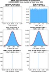 |
Fig. 1. Example of six DBEM input parameters with their corresponding uncertainties used in reverse modeling plotted in histograms (y-axis is density) as probability-density functions (PDFs) for the first event (January 8, 1997) from the analyzed CME list. The given uncertainties (99.7% confidence intervals or 3σ) are given above each plot (lower uncertainty < input value < upper uncertainty). The solid red line indicates the calculated normal distribution. Since the CME time, the angular half-width, and longitude of CME source position are set without the uncertainties, they are shown in the histograms as just a vertical line. In the reverse-modeling scheme, we allow all γ values with equal probability (no weight is applied); thus, the γ has continuous uniform distribution. |
2.3. Optimizing the reverse modeling
As described in Section 2.1, in order to find optimal γ, one searches for “perfect” DBEM solutions, i.e., a best match with the observed CME TT, for a predefined range of γ values. The optimal γ value is estimated as the median of the distribution of γ values leading to “perfect” DBEM solutions (where |ΔTTerr|≤1 h and |Δverr|≤75 km s−1). We hypothesize that the result for the optimal γ depends on the predefined range of γ values and that the true optimal γ can only be found if a suitable predefined range of γ values is used.
To test this hypothesis, we performed DBEMv3 reverse modeling on a sample of events described in Section 2.2 using different predefined ranges of γ values. More specifically, we varied the chosen γ ranges by 1) subsequently increasing the ranges of values (less computationally expensive, but operationally more complex) and 2) covering an extended range (more computationally expensive, but operationally simple). The γ ranges were chosen so that narrower ranges include larger γ ranges (e.g., the second range includes the entire first range etc.). The idea behind this was to understand how narrow γ ranges can influence the obtained γ values and their distributions compared to wider γ ranges. It would be expected that too-narrow γ ranges would not be able to find suitable γ values for certain events or would lead to shifted or skewed distributions compared to the wider ranges. In addition, one important goal was also to understand the trade-off between the range size and the resolution used, which is limited by the number of runs.
We define a total of four γ ranges, each of which is an extension of the previous one.
-
Range 1: 0.01–0.1 × 10⁻⁷ km−1, representing a very low drag, such as the one that occurs for, e.g., very fast CMEs and/or CMEs propagating in interplanetary space preconditioned by the passage of a high-speed stream or another CME (see, e.g., Temmer et al. 2017; Dumbović et al. 2019).
-
Range 2: 0.01–0.3 × 10⁻⁷ km−1, extending the previous range for typical drag experienced by CMEs (Vršnak et al. 2013).
-
Range 3: 0.01–1 × 10⁻⁷ km−1, extending the range for conditions with high drag, such as those encountered in, e.g., very slow CMEs (e.g., Dumbović et al. 2018b).
-
Range 4: 0.01–10 × 10−7 km−1, extending the range for extreme drag conditions, as in the tail of the drag parameter distribution for CMEs (see Vršnak et al. 2013).
The largest γ range, 4, was defined to cover all possible γ values that our sample can reach. According to Vršnak et al. 2013, statistical analysis, and some considerations, γ most often attains the values in the range of 0.2–2 × 10⁻⁷ km−1. In our case, we extended this range even further to 0.01–10 × 10−7 km−1. To substantiate the choice of this range, we performed an additional analysis, which is presented in Appendix B. Here, γ is calculated as a function of the mass of the CME, taking into account some assumptions about the cross-sectional area of the CME and the ambient solar-wind density. We show that the largest range used should be large enough to obtain all possible γ values for our sample of 31 events (see Figure B.1). For our sample, based on the CME mass values, the minimum γ value is 0.06 and the maximum γ value is 6.12 × 10⁻⁷ km−1. This is also supported by the analysis of Vršnak et al. 2008, where a much larger CME sample was used (several hundred CMEs) and the range of CME masses is similar to that of our CME sample. The inclusion of γ values over 10 × 10−7 km−1 would therefore possibly lead to physically infeasible γ values.
Although for the operational forecasting purposes it was shown that DBEM results converge quite rapidly after 10 000 DBM runs (Čalogović et al. 2021), for the purposes of reverse modeling, the number of runs was increased tenfold to 100 000 runs for all inputs to capture all possible random combinations for larger γ ranges. To test whether such a large number of runs is still sufficient, we also performed calculations with 500 000 runs to check the difference in results compared to the 100 000 runs with the same γ range (in this case, range 4 was used). For the purposes of reverse modeling, the γ ranges were represented by uniform distributions, as shown in Figure A.1 (upper right panel), instead of the commonly used normal (Gaussian) distributions for γ used in common operational DBEM mode (see Figure 1 in Čalogović et al. 2021).
2.4. Analysis of the applicability of the drag-based reverse modeling
The application of the reverse-modeling procedure using the four different γ ranges did not result in a solution for the optimal γ in seven out of 31 events (22%), even when the widest range of typical γ values (Vršnak et al. 2013) was used (range 4). We analyzed these events in more detail and found that for four events (events 1, 10, 29, and 31), the drag force was not the dominant force determining their propagation since these CMEs accelerate even at distances of 20 solar radii (RSUN). So, their propagation is not only determined by the drag force, which is the important assumption of the DBM that other forces such as acceleration can be neglected. To overcome this problem, the starting distance was increased by the trial-and-error method until a suitable starting distance was found that provided a perfect TT (similar to the method described in Sachdeva et al. 2015). Therefore, this distance was increased to 70 RSUN for events 1, 10, and 31 and to 50 RSUN for event 29. We also found that the initial CME speed v0 at 20 RSUN could be underestimated for events 26 and 27. This error could arise from the use of the second-order fit of the height-time measurements in the SOHO/LASCO CME catalogue (Gopalswamy et al. 2000), which shows very small deceleration in the LASCO FOV. In these cases, we used the value of the linear fit, which gave slightly different estimates of the CME speed. Accordingly, for events 26 and 27, the CME launch speed was changed, and the corresponding uncertainties were increased from 10% to 20%. However, even after these changes, the optimal γ was not found for events 13 and 27, indicating that these events might not be suitable for reverse modeling with the DBEM or DBM in general due to their complex dynamics (Temmer et al. 2011). Events 1, 10, 26, 27, 29, and 31, where the original input was changed, are marked with an asterisk in Table 1.
The results of reverse modeling and the search for the optimal γ parameter depend on the limitations of the DBM model, since the errors of other input parameters in the reverse modeling scheme are assumed to be constrained within predefined uncertainty intervals. Thus, γ values far away from the optimal value will result in highly overestimated or underestimated CME arrival times. Therefore, the calculation of the transit-time error (TTerr = TTDBEM − TTOBS) can serve as a metric for evaluating the applicability of the reverse modeling scheme, i.e., for whether or not a DBM solution for optimal γ can be found. We find that for a very large TTerr (TTerr > 30 h), the reverse modeling with the given uncertainties for five CME events (1, 26, 27, 29, 31) is not able to find the optimal γ parameter. For these events, the DBM is unable to capture the proper physics of CME propagation, or the input parameters are associated with large errors beyond assumed uncertainties. We were interested in how this lack of a physical result in DBEMv3 would be reflected in its “normal” operational mode, that is the kind of results the forecaster would obtain if it used the input for γ proposed by the DBEMv3 tool. For this purpose, we used the same inputs as in Table 1 for each event, except for the γ parameter. To estimate TTerr, γ was defined as a function of the speed of the CME, v0, as in the operational DBEMv3: for slow CMEs (v0 < 600 km s−1) γ = 0.5 × 10⁻⁷ km−1, for CMEs with regular speed (600 km s−1 ≥ v0≤ 1000 km s−1) γ = 0.2 × 10⁻⁷ km−1, and for fast CMEs (v0 > 1000 km s−1) γ = 0.1 × 10⁻⁷ km−1 with uncertainties ±Δγ of 0.1, 0.075, and 0.05 × 10⁻⁷ km−1, respectively. In this case, the distributions of the drag parameter defined by uncertainties were represented as normal distributions (as in the operational DBEMv3 mode and for all other input parameters). DBEMv3 was then run with 100 000 DBM ensemble members to obtain the median transit time (TTDBEM) and transit-time errors (TTerr) for each event.
The TTerr in operational DBEMv3 mode for all events in our CME sample are shown in Figure 2. Compared are the results for the TTerr with initial input (orange bars, input as in Table 1) and after changing the input for six events (blue bars, input marked with asterisk in Table 1), where a solution was then found. In all six cases where the optimal γ was not found in the initial input (events 1, 10, 26, 27, 29, and 31), the TTerr for the optimized input was massively reduced, as expected (e.g., up to 40 hours for event 1). It is important to note that in the operational mode DBEMv3 will always find some TT for a given γ, but this does not mean that reverse modeling would be able to provide a specific γ (i.e., converge) for a perfect TT. This depends on the difference between the initial CME speed and the solar-wind speed; the closer the two are, the more γ will diverge (see Section 3.3 or Vršnak et al. 2013). For all other events, the TTerr is the same, as expected (marked in dark green as overlapping results between the initial input marked in orange and the changed input marked in light blue).
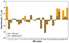 |
Fig. 2. Transit-time error (TTerr) in hours for the initial input (orange bars) and after changing input for specific events (light blue bars) for all 31 CMEs analyzed. Regions where TTerr overlaps for the two cases are marked in dark green (orange + blue = dark green). We note that for events where input was not changed, the overlap is 100%. |
2.5. Finding the optimal window for perfect arrival speed
Since DBM gives a prediction for two parameters – TT and vtar – to obtain a reliable optimal γ it is necessary to find the γ for both conditions together: perfect TT (where |ΔTTerr|≤1 h) and perfect vtar, where vtar matches the observed arrival speed vOBS within a given window. In previous studies – Paouris et al. (2021) and Čalogović et al. (2021) – this window was set to ±10 km s−1 (|vtar − vOBS|≤ 10 km s−1). However, this proved to be too narrow for our current sample of 31 CMEs, as no optimal γ was found for 17 of 31 events (∼55%). To find the optimal window for vtar, we used the largest γ range of 0.01–10 × 10−7 km−1 (range 4) and increased the window from 10 to 100 km s−1.
The results of the analysis to determine the optimal window for the perfect vtar are shown in Table 2. For comparison purposes, the first column (only TT) gives the optimal γ statistic for the perfect TT without any constraint in vtar. It is noted that despite the lack of constraint with perfect vtar, there are still two events (event 13 and 27) that did not result in an optimal γ for a perfect TT. All results for a perfect TT and vtar and different windows (±10, ±50, ±75, ±100) were also calculated separately for both observed arrival speeds: mean vOBS and peak vOBS (see Table 1). The second and third columns in Table 2 show the results for perfect TT and vtar with a window of ±10 km s−1, as used in the analyses of Paouris et al. (2021) and Čalogović et al. (2021). For this window, the number of events for which an optimal γ was found is small, and for 17 and 15 events, no optimal γ was found using mean vOBS and peak vOBS, respectively. The number of results found is also very small for mean vOBS (4749), compared to the number of all possible results under the condition of only perfect TT (75 988). However, in the case of peak vOBS, more results were found (31 309). The mean optimal γ is also much lower (e.g., 0.5 × 10⁻⁷ km−1 for the mean vOBS) than for other windows or only perfect TT (∼1.3 × 10⁻⁷ km−1). The next window with ±50 km s−1 (third and fourth columns in Table 2) obtained more results, with about 80% of events finding an optimal γ. As expected, the window with ±75 km s−1 (fifth and sixth columns in Table 2) obtained even more results, and in the case of mean vOBS, the optimal γ was not found in only four; moreover, the number of results found (73 129) was very close to the number of results with only perfect TT (75 988). Since the largest window of ±100 km s−1 (the last two columns in Table 2) did not yield a significant increase in the number of results or events with optimal γ, we selected the window of ±75 km s−1 as the most appropriate one. In addition, in this window, the mean vOBS yielded slightly more results than the peak vOBS, and there were fewer events where optimal γ was not found. Therefore, we chose the ±75 km s−1 window and the mean vOBS for the analysis in this study (indicated by bold values in the Table 2). This choice is also supported by the uncertainties used for the CME launch speed (v0), where the v0 mean for all events is 77 km s−1, comparable to the window for perfect vtar.
Statistics for found optimal γ.
Interestingly, the peak vOBS obtains more results with small windows (e.g., ±10 km s−1), and with larger windows (e.g., ±75 km s−1) the mean vOBS performs better in our sample. The difference is that the mean vOBS reflects better the CME propagation speed (this is under the assumption of self-similar expansion and assuming that the boundaries of the magnetic obstacle reflect it), and the peak vOBS accounts for both the propagation and expansion speed of the magnetic obstacle. This analysis also indicates that the window of only ±10 km s−1 for the perfect vtar used in previous studies (Paouris et al. 2021; Čalogović et al. 2021) may be set too low, and the results may be limited by this constraint.
3. Results
3.1. Analysis of different γ ranges
We first tested how limited γ ranges may affect the results of the optimal γ values found. As noted earlier, we are motivated by previous studies using DBM reverse modeling (Paouris et al. 2021; Čalogović et al. 2021), which used a constrained γ range of 0.01–0.59 × 10⁻⁷ km−1. For this purpose, DBEM results were restricted to those with a perfect TT and vtar, with a ±75 km s−1 window using the mean vOBS as the observed arrival speed (see Section 2.5).
The comparison of the calculated γ distributions and the optimal γ values depending on the four consecutively increasing ranges defined in Section 2.3 is shown in Figure A.1 for all events for which a solution to reverse modeling can be obtained. Additionally, to gain better insight into the γ distributions, skewness and kurtosis were also calculated (see Appendix C and Figure C.1).
As expected, by increasing the γ range, one increases the chance of finding the optimal γ for a given event. Thus, for the smallest γ range (0.01–0.1 × 10⁻⁷ km−1), the number of events in our CME sample for which the optimal γ was found was the lowest (ten events or 32.3%). For the next largest γ range (0.01–0.3 × 10⁻⁷ km−1), we found γ for a total of 20 events (64.5%). For an even larger range (0.01–1 × 10⁻⁷ km−1) we found γ for 26 events (83.9%), and for the largest range (0.01–10 × 10−7 km−1), γ was found for 27 events (87.1%). It may be possible to find γ for more events in our sample if the γ range were increased even further, however, there is a question of reliability of such a result, as it may not have the theoretical or observational support (see Appendix B and Vršnak et al. 2013).
In general, for about two thirds of the events we find a clear convergence of optimal γ (i.e., medians of γ distributions) to certain values by increasing the γ ranges (Figure A.1). The analysis of skewness (see Appendix C) also shows that by increasing the γ range we are more likely to capture the real optimal γ value with the median of the distribution. From Figure A.1 and skewness and kurtosis analysis (Figure C.1 in Appendix C), it can be concluded that limited γ ranges can produce skewed distributions that are shifted toward the direction of actual γ distribution, which is partially outside the analyzed γ range. On the other hand, very large γ ranges can produce γ distributions with very large tails (outliers).
Occasionally, using the correct γ range may yield more results than using the largest range due to the density of DBEM results produced in a given range. For example, in two cases (events 11 and 19), more results were found for optimal γ in range 2 (0.01–0.3 × 10⁻⁷ km−1) than in the largest range, 4 (0.01–10 × 10−7 km−1). In range 2, 97 and 22 optimal γ were found for events 11 and 19, respectively, while in range 4 only four and one optimal γ were found (Figure A.1). The reason for this is that the mean value for optimal γ fits range 2 very well, purely by chance (∼0.15 ×10⁻⁷ km−1). However, this was only observed for events where the number of γ found is very small.
3.2. The resolution’s impact on the optimal γ median values
As noted above, the limited number of DBEMv3 ensemble members or resolution may also affect the ability to find the optimal γ. Namely, once the distribution of possible γ values is found, the optimal γ is calculated as the median of the distribution. Therefore, the calculated optimal γ may depend on the number of γ values in the distribution (especially in asymmetric cases), which in turn depends on the number of ensemble members. To analyze this effect, we compared the results with the largest γ range (0.01–10 × 10−7 km−1) using 100 000 ensemble members per event with the results of calculations using 500 000 ensemble members (for the same input). By using the larger number of ensemble members (in this case, five times larger), we found no significant difference in the results. The mean absolute median difference in γ was 0.01 with a standard deviation of 0.018 × 10⁻⁷ km−1, which is a negligible difference compared to other model and input uncertainties. The obtained 95th percentile γ ranges did not change significantly either and had average differences of about 0.01, with standard deviations smaller than 0.03 × 10⁻⁷ km−1 and maximum differences in some cases as large as 0.08 × 10⁻⁷ km−1. Thus, we conclude that 100 000 ensemble members are fully sufficient to obtain the correct γ distributions in all analyzed γ ranges. Interestingly, the analysis using 500 000 ensemble members also yielded one optimal γ (0.22 × 10⁻⁷ km−1) for event 1, where analysis using 100 000 ensemble members found no results for an optimal γ. Therefore, the larger number of ensemble members may make a difference if just a few optimal γ results are found. This was also the case for events 11 and 19, where the calculations with 500 000 ensemble members yielded 11 and two more optimal γ, respectively, than in the case of 100 000 ensemble members. Since such results were only obtained at the extreme edge of the γ distributions constrained by perfect TT and vtar, such results may not be very reliable. On the other hand, we note that the overall statistics for our CME sample would not change significantly even if there were a slightly smaller number of ensemble members (e.g., with 50 000 ensemble members, as previously reported in Čalogović et al. 2021 and Paouris et al. 2021).
3.3. Analysis of optimal γ with largest γ range (0.01–10 × 10−7 km−1)
The results of finding the optimal γ for a perfect TT and vtar with a ±75 km s−1 window employing the mean vOBS and using the widest γ range 0.01–10 × 10−7 km−1 are shown as boxplots for all analyzed CMEs in Figure A.2. For better visibility, the entire γ range in Figure A.2 is divided into two subplots: the top one shows γ for 1–10 and the middle one shows γ for 0.01 − 1 × 10⁻⁷ km−1. The third subplot from the bottom with bars shows the number of γ solutions found for each event in our CME sample. In general, the number of γ solutions found was less than 1% for more than 70% of the events, relatively to the total number of ensemble members (100 000) calculated for each event.
For the majority of events analyzed (∼61%, or 19 total), the optimal γ was found to be in the range of 0.01–0.5 × 10⁻⁷ km−1, which is the common operational DBEMv3 range. Notably, for the previously used restricted γ range of 0.01–0.59 × 10⁻⁷ km−1 (Paouris et al. 2021; Čalogović et al. 2021), γ values were obtained for 25 events, or in 81% of analyzed events, and the median γ values (< 0.6 × 10⁻⁷ km−1) were found in this range for 19 events (61%). Compared to the largest γ range (0.01 − 10 × 10−7 km−1), which obtained γ values for 87% of events, this is a rather small increase of 6% (two events). However, the median optimal γ values found in the largest range were outside the previously restricted γ range for eight events (26%). Interestingly, event 24 (CME on 11.04.2013) was also used in the analysis of Paouris et al. (2021) and Čalogović et al. (2021) (as event 1). The reverse modeling analysis in Paouris et al. (2021) yielded an optimal γ median value of 0.38 × 10⁻⁷ km−1, while in this analysis for the same event and the largest γ range employed the median γ value is 1.12 × 10⁻⁷ km−1. However, the spread of γ for event 24 is quite large, with the minimum value being 0.58 × 10⁻⁷ km−1, which would also possibly be caught in the the Paouris et al. (2021) range. The reasons for the larger discrepancy could be due to the use of the different sized vtar window, with ±75 km s−1 and slightly different input parameters, as well as the slightly different methods and the fact that the calculations were performed with a newer and updated version of DBEM.
An important quantity governing the CME propagation in the DBM equations is the difference between the CME launch speed and the solar-wind speed (v0 − w), since the DBM CME kinematics is governed solely by the MHD aerodynamic drag force and the drag acceleration is given as ad = −γ(v − w)|v − w| (Cargill 2004; Vršnak et al. 2010, 2013). With this in mind, the difference v0 − w was calculated for each event from our sample and is shown in Figure 3. The difference v0 − w determines whether the CME is accelerated or decelerated, and it is responsible for the kinematic profile of the CME. Thus, with the given uncertainties, v0 − w determines the capability and the range in which optimal γ is found. For example, in the case of v0 − w ≈ 0, γ can in principle take on very large arbitrary values so that TTDBEM matches TTOBS.
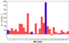 |
Fig. 3. Difference between CME launch speed and solar-wind speed (v0 − w) in km s−1. The blue bars denote events that did not find any optimal γ value. |
The blue bars in Figure 3 represent the events (CME 1, 13, 20, 27) that did not find an optimal γ in any range. For three events (1, 13, and 27), the v0 − w difference is quite small (v0 − w < 250 km s−1) and probably due to larger input and/or model uncertainties leading to larger TTerr, it was not possible to find the optimal γ with the reverse modeling. This is illustrated in Figure A.3, which shows TTerr for results constrained by perfect vtar with a ±75 km s−1 window. The TTerr intersecting the gray shaded area represents the results corresponding to the perfect TT, where the optimal γ was found for a given event (marked with blue boxes in Figure A.3). The events that do not overlap with the gray shaded area (indicated by yellow boxes) correspond to four CMEs for which no optimal γ was found. Event 20 is a very fast CME (v0 = 2265 km−1, see Table 1) and has one of the largest negative TTerrs (underestimation) and quite a low observed vtar compared to v0 (mean vOBS = 498 km s−1). This could indicate a possible larger overestimation of its launch speed that is not covered by the uncertainties used (10%). Similar examples of fast events were also found in Čalogović et al. (2021) when analyzing the larger Richardson & Cane 146 CME-ICME pair sample, where several faster events (e.g., Halloween solar storms in 2003) were also associated with very large errors in predicted vtar.
To further distinguish different types of events in our CME sample (Table 1), we divided them into five distinct groups based on the γ values obtained in the 0.01–10 × 10−7 range and some common characteristics (the numbers in parentheses correspond to the CME event number):
-
Group 1, γ found in the 0.01–0.3 × 10⁻⁷ km−1 range (events: 5, 9, 11, 15, 17, 19, 22, 26, 28, 29, 30, 31)
-
Group 2, γ found in the 0.3–0.6 × 10⁻⁷ km−1 range (events: 3, 4, 7, 8, 18, 21)
-
Group 3, γ found in the 1–10 × 10−7 km−1 range (events: 2, 23)
-
Group 4, γ found in the 0.01–10 × 10−7 km−1 range (events: 6, 10, 12, 14, 16, 24, 25)
-
Group 5, no optimal γ found (events: 1, 13, 20, 27)
We note that the five groups above are different from the increasing γ ranges defined in Section 2.3. The statistics for the five event groups listed above and for all events together (total) are shown in Table 3. It shows the median optimal γ and the v0 − w difference with the corresponding 95th percentile ranges. The TTerr obtained with DBEM using γ input ranges as in normal operating mode are also given in Table 3. Overall, the median optimal γ value is 1.33 × 10⁻⁷ km−1 and the TTerr is biased toward the negative values (underestimated TTDBEM) with a mean of −3.10 hours and a mean |TTerr| of 10.62 hours. All CMEs in our sample according to DBM are decelerated since v0 − w > 0, with v0 − w values ranging from a few hundred to about 2000 km s−1; the only exception was event 23, where v0 − w < 0 (v0 − w = −64 km s−1) and the corresponding CME is accelerated (see Figure 3).
A detailed analysis of the five different CME groups as defined above can be found in Appendix D. In comparison, the first group obtained γ values for 39% of events in low- and normal-drag ranges (0.01–0.3 × 10⁻⁷ km−1), with relatively small and mostly positive TTerrs (overestimated TT) of under ten hours and larger differences in v0 − w (mean 389 km s−1), while the second group with increased drag (0.3–0.6 × 10⁻⁷ km−1, 19% events) showed much larger negative TTerrs (underestimated TT, mean TTerr = −13.16 hours). The third group with extreme drag (1 − 10 × 10−7 km−1), which consists of only two events (6%), is characterized by the largest TTerr (mean TTerr = 22.12 hours) and a small v0 − w difference (mean 74 km s−1). The fourth group, in which the γ values were essentially found in the entire analyzed drag range (0.01–10 × 10−7 km−1, 22% events), is characterized by a small TTerr. The fifth group yielded no γ values in the analyzed range and, as expected, has a very large TTerr (mean |TTerr| = 21.77 hours).
Interestingly, out of the nine CMEs that obtained γ values in the range of the extreme γ values (1–10 × 10−7 km−1), for four CMEs (44%) the extreme γ values were also obtained as a function of their CME mass, which was low compared to other events (see Figure B.1 in Appendix B). However, due to the relatively small CME sample and the errors that may affect the γ values obtained with reverse modeling, it is difficult to say that this is a significant result.
The analysis in the largest γ range (0.01–10 × 10−7 km−1) was also repeated using the peak vOBS instead of the mean vOBS as the value for the observed arrival speed with the same window of ±75 km s−1 for perfect vtar (see Section 2.5). For a total of 18 events (58%), no difference was found in the results for optimal γ. For three events (CME 13, 20, and 27), optimal γ for a perfect TT and vtar was also not found, as was the case with the mean vOBS analysis. Interestingly, for event 1 the peak vOBS led to 231 results for optimal γ, with a mean γ value of 0.14 × 10⁻⁷ km−1, compared to zero with the mean vOBS. In contrast, an analysis with peak vOBS did not yield an optimal γ for events 7 and 11. For six events, the differences between the optimal γ found using the mean and the peak vOBS were very small (< 0.035 × 10⁻⁷ km−1), with three events having a difference less than 0.001 × 10⁻⁷ km−1. The larger difference was only observed in event six, where the peak vOBS found 3800 more results for an optimal γ, resulting in a median γ of 1.71 × 10⁻⁷ km−1 (−0.6 difference compared to the mean vOBS). To summarize, the overall differences in median and mean γ when using the mean or peak vOBS are quite small (see also Table 2), and the use of the peak instead of the mean vOBS would not significantly change the results of this study.
In summary, we find that the difference between the CME launch speed and the solar-wind speed, v0 − w, may affect the size of the optimal γ distributions and the ability to find an optimal γ with reverse modeling. To illustrate this, in Figure 4 we show the dependence of the obtained optimal γ with the largest γ range used (0.01–10 × 10−7 km−1) on the v0 − w difference. For v0 − w differences smaller than about 200 km s−1, the medians of the γ distributions (shown as red crosses in Figure 4) can take very large values (e.g., γ > 1 × 10⁻⁷ km−1), and the corresponding distributions are very long (shown as 95th percentile intervals with blue bars). This is in agreement with theoretical expectations, where in the case of constant drag and very small v0 − w we would expect the reverse-modeling method not to converge. This is evident for events 14 and 16, where despite very small v0 − w, an optimal γ was found with reverse modeling in all four increasing γ ranges. For these two events, the TTerr in operational DBEMv3 mode was very small (TTerr < 5 h), which made possible to find optimal γ values. However, the very small v0 − w caused the very large scatter of γ values in the analyzed range, reflecting the diverging aspect of the method. On the other hand, events 13 and 27, which also have a small v0 − w range, have a much larger TTerr in DBEMv3 operational mode. For these events, no suitable γ values exist for the given set of input parameters, either due to unreliable input or the complexity of the method making DBM unsuitable to describe the underlying CME propagation physics. Therefore, we find that the constraining factors of the reverse-modeling method, when it may not find reliable results, are as follows: 1) v0 − w is small; 2) input values are unreliable; and 3) there are physical limitations to DBM as a simple analytical model (e.g., CME-CME interactions, influence of high-speed streams). We note that it is not entirely clear how small v0 − w needs to be in order for the method to diverge. Although for this particular sample v0 − w < 200 km s−1 seems to be the threshold above which there is no divergence, not all of the events with v0 − w < 200 km s−1 show divergence. The detailed analysis of the conditions leading to the divergence is, however, beyond the scope of this study.
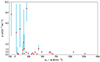 |
Fig. 4. Dependence of optimal γ found on the difference between CME launch speed and solar-wind speed (v0 − w). The red crosses denote the median of the γ values, and the blue bars show the 95th percentile intervals. |
4. Summary and conclusions
The drag-based ensemble model v3 tool (DBEMv3 tool, Čalogović et al. 2021) is a simple space-weather-forecast tool, which, through application of the uncertainties and ensembles on the widely used analytical drag-based model (DBM, Vršnak et al. 2013), provides distributions and confidence intervals as results. It calculates the most probable arrival time and speed of CMEs at Earth or a specific target (planets, spacecraft) in the Solar System. Some of the DBEMv3 input parameters are not easy to measure or to obtain directly, such as the drag parameter γ. To analyze what values the drag parameter γ can take for different CMEs, optimal γ can be calculated, giving the perfect TT within ± one hour of the actual observed transit time (TTOBS) and perfect vtar within a ±75 km s−1 window using the inverse-modeling method (Paouris et al. 2021; Čalogović et al. 2021). We tested the performance and limitations of such a procedure.
For this purpose, we used a list of 31 CMEs (see Table 1) compiled by Martinić et al. (2023) during the period from 1997 to 2018. To determine the perfect vtar, two observed arrival speeds were extracted: mean and peak vOBS. The mean vOBS represents the mean speed within the magnetic-obstacle (MO) part, and the peak vOBS is the impact speed at the beginning of the MO in the ICME, or the leading edge speed. Using these two observed arrival speeds, we searched for the optimal window defining the perfect vtar by gradually increasing the window from ±10 to ±100 km s−1. It was found that the optimal window is ±75 km s−1, which is also supported by the fact that the mean uncertainty for all evens in the CME launch speed is 77 km s−1. This suggests that the previously used window of ±10 km s−1 in Paouris et al. (2021), Čalogović et al. (2021) may be too narrow. In our sample, the analysis with mean vOBS yielded more optimal γ results than the peak vOBS, although for the whole sample there were no significant differences if the mean or the peak vOBS was used with a window of ±75 km s−1.
To test the possible effects of using the very restricted γ input ranges on the optimal γ values found, as might be the case in previous studies (Paouris et al. 2021; Čalogović et al. 2021), we analyzed the four increasing γ input ranges. The largest γ range in this study (0.01–10 × 10−7 km−1) was 16 times larger compared with the analysis of Paouris et al. (2021) and Čalogović et al. (2021). By optimizing several input parameters in the initial DBEMv3 tool input, it was possible to reduce the number of CMEs for which the optimal γ search failed. However, no physical solutions could be found for four events, most probably due to the fact that DBM is not able to capture the physics of those events (similarly to what was found previously by Vršnak et al. 2013). In two of these events, no optimal γ was found due to the fact that the predicted DBEM vtar was outside the prefect vtar window.
As expected, as the γ input range increased, as did the chance of finding the optimal γ for a given event. About two thirds of the analyzed CMEs in our sample showed a clear convergence to a particular distribution and median value with increasing γ range. In addition, the calculated skewness and kurtosis for each event and different γ ranges showed significantly shifted distributions of the optimal γ for those events where the actual γ was close to or slightly outside the restricted γ range. On the other hand, the very large γ ranges showed distributions with a very wide tail (high skewness) for some events.
We found that the limited number of DBEMv3 tool ensemble members did not significantly affect the determination of the optimal γ for the largest γ input ranges when a sufficient number of ensemble members is used. The tests where the number of ensemble members was increased fivefold (from 100 000 to 500 000) showed no significant differences in the results. Thus, we conclude that the chosen number of ensemble members (100 000) was sufficient to find the optimal γ values.
To determine whether the optimal γ can be found with the DBEMv3 tool, the TTerr were calculated as TTDBEM − TTOBS for each CME using the DBEMv3 tool in its operational mode with the proposed normal input for γ and their corresponding uncertainties as a function of the speed of the CME (e.g., for slow CMEs, v0< 600 km s−1γ = 0.5 × 10⁻⁷ km−1 with uncertainties ±Δγ of 0.1 × 10⁻⁷ km−1). This allowed the estimation of the TTerr that the user would obtain using the operational DBEMv3 tool with a proposed arbitrary γ value.
Medians of optimal γ were found to be in the common operational DBEMv3 γ range of 0.01–0.5 × 10⁻⁷ km−1 for about two thirds of all CMEs analyzed. For two events, a very large optimal γ was found with a median γ of 8.21 × 10⁻⁷ km−1. Common to these events where a large γ was found was a smaller difference between the CME launch speed, v0 and the solar-wind speed, w compared to other events (v0 − w ∼ 70 km s−1) and moderate TTerr. Since v0 − w in quadratic form multiplied by γ defines the main DBM drag equation of motion, the corresponding γ must be very large if v0 − w is small to balance the larger TTerr. This was also the case for the two events that did not obtain any optimal γ in the largest γ range due to larger TTerr than for the group of events that obtained the extreme drag values.
We find that the constraining factors of the reverse-modeling method, when it may not find reliable results, are as follows: 1) when v0 − w is small; 2) unreliable input; and 3) physical limitations of DBM as a simple analytical model (e.g., CME-CME interactions, influence of high-speed streams).
In summary, our analysis shows the importance of using an appropriate γ input range to find the optimal γ values using a reverse-modeling method. Using too narrow γ ranges can lead to skewed distributions of possible γ values or to finding no solutions at all, while too large γ ranges can lead to physically infeasible optimal γ values. An important quantity that affects finding optimal γ values is the difference in v0 − w. If this quantity is small (CME launch speed is close to the solar-wind speed), the corresponding optimal γ can easily take on very large values, which may not be physically plausible.
Acknowledgments
M.D., K.M. and B. V. acknowledge the support by the Croatian Science Foundation under the project IP-2020-02-9893 (ICOHOSS). K.M. acknowledges support by Croatian Science Foundation in the scope of Young Researches Career Development Project Training New Doctoral Students. M.D. and M.T. acknowledge support from the Austrian-Croatian Bilateral Scientific Project “Analysis of solar eruptive phenomena from cradle to grave”.
References
- Burkepile, J. T., Hundhausen, A. J., Stanger, A. L., St. Cyr, O. C., & Seiden, J. A. 2004, J. Geophys. Res.: Space Phys., 109, A03103 [NASA ADS] [CrossRef] [Google Scholar]
- Čalogović, J., Dumbović, M., Sudar, D., et al. 2021, Solar Phys., 296, 114 [CrossRef] [Google Scholar]
- Cargill, P. J. 2004, Sol. Phys., 221, 135 [Google Scholar]
- Cargill, P. J., Chen, J., Spicer, D. S., & Zalesak, S. T. 1996, J. Geophys. Res., 101, 4855 [NASA ADS] [CrossRef] [Google Scholar]
- Colaninno, R. C., & Vourlidas, A. 2009, ApJ, 698, 852 [NASA ADS] [CrossRef] [Google Scholar]
- Dumbović, M., Čalogović, J., Vršnak, B., et al. 2018a, ApJ, 854, 180 [CrossRef] [Google Scholar]
- Dumbović, M., Heber, B., Vršnak, B., Temmer, M., & Kirin, A. 2018b, ApJ, 860, 71 [CrossRef] [Google Scholar]
- Dumbović, M., Guo, J., Temmer, M., et al. 2019, ApJ, 880, 18 [Google Scholar]
- Dumbović, M., Čalogović, J., Martinić, K., et al. 2021, Front. Astron. Space Sci., 8, 58 [Google Scholar]
- Gopalswamy, N., Lara, A., Lepping, R. P., et al. 2000, Geophys. Res. Lett., 27, 145 [NASA ADS] [CrossRef] [Google Scholar]
- Gopalswamy, N., Yashiro, S., Michalek, G., et al. 2009, Earth Moon Planets, 104, 295 [NASA ADS] [CrossRef] [Google Scholar]
- Hess, P., & Zhang, J. 2014, ApJ, 792, 49 [NASA ADS] [CrossRef] [Google Scholar]
- Hinterreiter, J., Magdalenic, J., Temmer, M., et al. 2019, Sol. Phys., 294, 170 [NASA ADS] [CrossRef] [Google Scholar]
- Kay, C., Mays, M. L., & Verbeke, C. 2020, Space Weather, 18, e02382 [CrossRef] [Google Scholar]
- King, J. H., & Papitashvili, N. E. 2005, J. Geophys. Res.: Space Phys., 110, A02104 [CrossRef] [Google Scholar]
- Leblanc, Y., Dulk, G. A., & Bougeret, J.-L. 1998, Sol. Phys., 183, 165 [NASA ADS] [CrossRef] [Google Scholar]
- Lugaz, N., Manchester, W. B., I., & Gombosi, T. I. 2005, ApJ, 627, 1019 [NASA ADS] [CrossRef] [Google Scholar]
- Martinić, K., Dumbović, M., Čalogović, J., et al. 2023, A&A, 679, A97 [NASA ADS] [CrossRef] [EDP Sciences] [Google Scholar]
- Mays, M. L., Taktakishvili, A., Pulkkinen, A., et al. 2015, Sol. Phys., 290, 1775 [CrossRef] [Google Scholar]
- Owens, M., & Cargill, P. 2004, Ann. Geophys., 22, 661 [NASA ADS] [CrossRef] [Google Scholar]
- Paouris, E., Čalogović, J., Dumbović, M., et al. 2021, Solar Phys., 296, 12 [NASA ADS] [CrossRef] [Google Scholar]
- Riley, P., Mays, M. L., Andries, J., et al. 2018, Space Weather, 16, 1245 [NASA ADS] [CrossRef] [Google Scholar]
- Sachdeva, N., Subramanian, P., Colaninno, R., & Vourlidas, A. 2015, ApJ, 809, 158 [NASA ADS] [CrossRef] [Google Scholar]
- Samara, E., Pinto, R. F., Magdalenić, J., et al. 2021, A&A, 648, A35 [EDP Sciences] [Google Scholar]
- Sudar, D., Vršnak, B., Dumbović, M., Temmer, M., & Čalogović, J. 2022, A&A, 665, A142 [NASA ADS] [CrossRef] [EDP Sciences] [Google Scholar]
- Temmer, M. 2021, Liv. Rev. Sol. Phys., 18, 4 [NASA ADS] [CrossRef] [Google Scholar]
- Temmer, M., Rollett, T., Möstl, C., et al. 2011, ApJ, 743, 101 [NASA ADS] [CrossRef] [Google Scholar]
- Temmer, M., Vršnak, B., Rollett, T., et al. 2012, ApJ, 749, 57 [NASA ADS] [CrossRef] [Google Scholar]
- Temmer, M., Reiss, M. A., Nikolic, L., Hofmeister, S. J., & Veronig, A. M. 2017, ApJ, 835, 141 [Google Scholar]
- Thernisien, A. 2011, Astrophys. J. Suppl., 194, 33 [NASA ADS] [CrossRef] [Google Scholar]
- Thernisien, A. F. R., Howard, R. A., & Vourlidas, A. 2006, Astrophys. J., 652, 763 [NASA ADS] [CrossRef] [Google Scholar]
- Thernisien, A., Vourlidas, A., & Howard, R. A. 2009, Solar Phys., 256, 111 [CrossRef] [Google Scholar]
- Verbeke, C., Mays, M., Kay, C., et al. 2022, Adv. Space Res., 72, 5243 [Google Scholar]
- Vourlidas, A., Subramanian, P., Dere, K. P., & Howard, R. A. 2000, ApJ, 534, 456 [NASA ADS] [CrossRef] [Google Scholar]
- Vourlidas, A., Howard, R. A., Esfandiari, E., et al. 2010, ApJ, 722, 1522 [NASA ADS] [CrossRef] [Google Scholar]
- Vourlidas, A., Patsourakos, S., & Savani, N. P. 2019, Philos. Trans. R. Soc. Lond. Ser. A, 377, 20180096 [NASA ADS] [Google Scholar]
- Vršnak, B., & Žic, T. 2007, A&A, 472, 937 [NASA ADS] [CrossRef] [EDP Sciences] [Google Scholar]
- Vršnak, B., Ruždjak, D., Sudar, D., & Gopalswamy, N. 2004, A&A, 423, 717 [NASA ADS] [CrossRef] [EDP Sciences] [Google Scholar]
- Vršnak, B., Vrbanec, D., & Čalogović, J. 2008, A&A, 490, 811 [NASA ADS] [CrossRef] [EDP Sciences] [Google Scholar]
- Vršnak, B., Žic, T., Falkenberg, T. V., et al. 2010, A&A, 512, A43 [CrossRef] [EDP Sciences] [Google Scholar]
- Vršnak, B., Žic, T., Vrbanec, D., et al. 2013, Sol. Phys., 285, 295 [Google Scholar]
- Zhang, J., Temmer, M., Gopalswamy, N., et al. 2021, Prog. Earth Planet. Sci., 8, 56 [CrossRef] [Google Scholar]
Appendix A: Figures
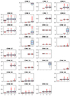 |
Fig. A.1. Dependence of the optimal γ on 4 consecutively increasing γ ranges for all events where γ is found via reverse modeling (i.e. all CMEs except CME 1, 13 , 20 and 27 where no optimal γ was found). y-axis represents the γ value in ×10−7 km−1, whereas on the x-axis four γ ranges are given: 1) 0.01–0.1, 2) 0.01–0.3, 3) 0.01–1, and 4) 0.01–10 ×10−7 km−1. The boxes denote the interquartile range (IQR) limited by the 1st quartile (Q1: 25th percentile) and the 3rd quartile (Q3: 75th percentile), where 50% of the data are found. The median is represented by a red line, and the notches show the 95% confidence interval of the median. Whisker ranges define minimum and maximum values, defined as Q1 − 1.5 * IQR and Q3 + 1.5 * IQR, respectively. Outliers are marked with the red dots. |
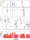 |
Fig. A.2. Upper panels show boxplots for the optimal γ with perfect TT and vtar found in 0.01–10×10−7 km−1 range for all CME events. Two separate panels are used due to extensiveness of the γ range. Boxes denote the interquartile range (IQR) limited by the 1st quartile (Q1: 25th percentile) and the 3rd quartile (Q3: 75th percentile) where 50% of the data were found. The median value is represented by a red line, and the notches show the 95% confidence interval of the median. Whisker ranges define minimum and maximum values, defined as Q1 − 1.5 * IQR and Q3 + 1.5 * IQR, respectively. Outliers are marked with the red dots. The bottom panel shows the number of reverse modeling results (γ values) found for each event (note that we use the logarithmic y-axis). |
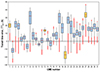 |
Fig. A.3. Transit time error (TTerr) in hours for all CME events calculated with the largest γ range (range 4) and constrained by perfect arrival speed in ±75 km s−1 window. The gray shaded area shows the interval for perfect TT (|ΔTTerr|≤1 h). Events for which an optimal γ was found are marked with blue boxes and those for which no γ was found are marked with yellow boxes. All other labels are the same as in the Figure A.2. |
Appendix B: Determining the limits of the largest γ range
Since drag parameter γ is difficult to determine by direct measurements, an additional analysis was performed using the CME masses to reliably determine the entire γ range in which we can expect the γ values for our sample. γ can be defined with the following equation from Vršnak et al. 2008, 2013:
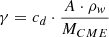
where cd is the dimensionless drag coefficient, A is the effective CME area perpendicular to the propagation direction, ρw is the ambient solar wind density and MCME is the CME mass. Assuming that cd is constant and equal to 1 (Cargill 2004), A for a typical partial/full halo CME is ∼ 1014 km2 at 20 RSUN (Vršnak et al. 2013), and ρw at the same distance can be approximated with the density model of Leblanc et al. 1998, therefore the calculated γ depends only on the CME mass.
For this purpose, the CME masses for our sample were taken from the SOHO/LASCO CME catalogue (Gopalswamy et al. 2009). The mass was missing for only two events (11, 26). At this point, it should be noted that our sample of full/partial halo CMEs directed towards Earth all have poor mass estimates due to sky-plane assumption (Vourlidas et al. 2000, 2010). However, the mass estimates can be underestimated by a factor of up to ∼ 2 (Vourlidas et al. 2000; Lugaz et al. 2005; Colaninno & Vourlidas 2009).
The calculated γ values as a function of CME mass for our CME sample are shown in Figure B.1. The heaviest CMEs have the smallest γ values (minimum 0.06 ×10⁻⁷ km−1), while the lightest CMEs have the largest γ values (maximum 6.12 ×10⁻⁷ km−1) and fit well into the largest γ range 4 selected for this analysis. Furthermore, the calculated γ as a function of CME mass might be overestimated because the CME masses are underestimated, confirming that a range above 10 ×10−7 km−1 for γ is probably not physically feasible.
Appendix C: Analyzing obtained γ distributions with skewness and kurtosis
To gain better insight into the γ distributions obtained for different γ ranges, the skewness and kurtosis (see Figure C.1) was calculated for each distribution. The skewness (left panels in Figure C.1) measures the symmetry of the distribution, while the kurtosis (right panels in Figure C.1) determines the heaviness of the distribution tails. When skewness is negative, the tail of the distribution is longer on the left side and when it is positive, the tail of the distribution is longer on the right side. Kurtosis describes the peaked-ness of the distribution, where a high kurtosis value is an indicator that the data has strong outliers and a low kurtosis value is an indicator that the data has no outliers. In a perfect normal distribution, one would expect the skewness to have values around 0 and the kurtosis to have values around 3.
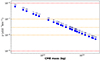 |
Fig. C.1. Calculated drag parameter γ as a function of the CME masses in our sample shown in log-log plot. The CME number corresponding to our events list is indicated above the plotted dots. The red dotted lines denote the full range of γ used in this study (0.01 – 10 ×10−7 km−1) and the orange dotted lines correspond to the boundaries of the restricted γ ranges: 0.1, 0.3 and 1 ×10⁻⁷ km−1. |
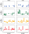 |
Fig. C.2. Skewness (left panels) and kurtosis (right panels) of γ distributions calculated for all events and different four γ ranges: 1) 0.01–0.1 (first row, blue bars), 2) 0.01–0.3 (second row, green bars), 3) 0.01–1 (third row, orange bars), and 4) 0.01–10 ×10−7 km−1 (last row, red bars). |
The calculated skewness (left panels in Figure C.1) shows the gradual transition from negative values to positive values with increasing γ ranges. This means that the peaks of the distributions in limited small γ ranges are shifted toward the highest values (negative skewness), while the actual γ median values are outside this range as determined in larger γ ranges. This means that by increasing the γ range, there is a greater chance that the real optimal γ range will be captured.
By increasing the γ range we first see an increase in the optimal γ (for range 3), followed by the decrease of the optimal value for the largest γ range. The possible explanation lies in the decrease of the resolution which inevitably comes with increasing the γ range while leaving the number of runs (ensemble members) unchanged. However, we note that that this is clearly a minor effect, as the medians found in ranges 3 and 4 are not significantly different (as indicated by the overlapping notches of the box plot). This effect is accompanied by an increase in positive skewness, i.e. the distribution becomes more asymmetric with tendency towards lower γ values.
Similar effect in the skewness can be observed in several other events (6, 16, 24, 25) for which optimal γ is found in the very large drag range. For these events large positive skewness was obtained for the largest γ range (lowest left panel in Figure C.1). These events also showed a high positive kurtosis (lowest right panel in Figure C.1), suggesting that the tails of the γ distribution are quite long. We note that asymmetry of the γ distribution for these events did not affect the convergence of the median towards the optimal γ value.
To summarise, γ ranges that are too narrow can lead to skewed distributions that are shifted in the direction of the actual γ distribution, which in turn may lie outside restricted range. However, larger γ ranges can produce γ distributions with large tails and outliers.
Appendix D: Analysis of five distinct CME groups based on the γ values obtained in the largest 0.01 – 10 ×10−7 km−1 range
Here we present in more detail five different CME groups based on the different γ value ranges determined using reverse modeling (as defined in Section 3.3). The summary of all statistics for these five groups and the obtained γ values, v0 − w difference and TTerr can be found in Table 3.
For the first group consisting of largest number of events (see Table 3), we find optimal γ in the low-drag and normal drag ranges (∼39% or 12 events). Common to all these events is a rather small TTerr below 10 hours (95th percentile range is −6.18 to +10.80 hours) and mostly with positive TTerr values (overestimated TTDBEM) with the median TTerr for all events of +3.08 hours (see Table 3). Three CMEs (11, 15, 19) in this group were fast events with CME launch speeds around 1000 km s−1 or more, for which the lower γ values (γ < 0.3 ×10⁻⁷ km−1) would also be expected. We note again that very few results (< 5) for optimal γ were found in events 11 and 19 and the results for these events may not be entirely reliable. According to Table 3, the first group of events also shows the lowest mean |TTerr| of 5.50 hours. The first group of events is also found to have a larger difference in v0 − w with a mean of 389 km s−1 and a larger 95th percentile range compared to the other groups (64 – 1112 km−1).
The second group of events has an optimal γ found in the range corresponding to the somewhat increased drag (six events in total). Common to this group is the large mean TTerr of −13.16 hours, with five of six events having negative TTerr values. Two events (7 and 18) are fast CMEs (v0 > 1000 km s−1), for which a lower γ (∼ 0.1 ×10⁻⁷ km−1) should be expected. This indicates that for these events the speed-scaled γ values as suggested by the normal operational mode of DBEMv3 may not be suitable.
The third group of events has an optimal γ in the range of extreme drag conditions, 1–10 ×10−7 km−1 and consists of only 2 events. Common to this group is the large TTerr with a mean absolute |TTerr| of 22.12 hours (Table 3 and Figure 2) and the rather small differences in v0 − w with a mean of 74 km s−1 (Figure 3). Moreover, event 23 was the CME accelerating during its transit, with solar wind speed greater than the CME launch speed. Since TTerr is large and the difference in v0 − w is very small, the resulting optimal γ can take very large values.
The fourth group of events consists of seven events that were found in the very extended drag range (0.01–10 ×10−7 km−1), where the 95th percentile range of median γ for all events was between 0.31 and 4.75 ×10⁻⁷ km−1. These events show smaller TTerr with a mean TTerr of −5.52 hours and a mean absolute |TTerr| of 6.83 hours. The difference in v0 − w is slightly larger than for the third group of events with a mean of 151 km s−1. Since TTerr is not as large as in the third and second group, it was possible to obtain the entire wide range of γ that yielded the perfect TT with some tendency toward the higher γ values (mean γ = 2.10 ×10⁻⁷ km−1).
The last and fifth group of events corresponds to four events for which no optimal γ was found. As expected, TTerr in this group are very large with a mean absolute |TTerr| of 21.77 hours. For two events (13 and 27), no optimal γ could be found in the given range of physically reasonable γ values because of the large TTerr and the small difference in v0 − w (mean 100 km s−1). For the other two events (1 and 20) either no perfect γ was found, due to the constraint with perfect vtar in the ±75 km s−1 window as described above.
All Tables
All Figures
|
Fig. 1. Example of six DBEM input parameters with their corresponding uncertainties used in reverse modeling plotted in histograms (y-axis is density) as probability-density functions (PDFs) for the first event (January 8, 1997) from the analyzed CME list. The given uncertainties (99.7% confidence intervals or 3σ) are given above each plot (lower uncertainty < input value < upper uncertainty). The solid red line indicates the calculated normal distribution. Since the CME time, the angular half-width, and longitude of CME source position are set without the uncertainties, they are shown in the histograms as just a vertical line. In the reverse-modeling scheme, we allow all γ values with equal probability (no weight is applied); thus, the γ has continuous uniform distribution. |
| In the text | |
|
Fig. 2. Transit-time error (TTerr) in hours for the initial input (orange bars) and after changing input for specific events (light blue bars) for all 31 CMEs analyzed. Regions where TTerr overlaps for the two cases are marked in dark green (orange + blue = dark green). We note that for events where input was not changed, the overlap is 100%. |
| In the text | |
|
Fig. 3. Difference between CME launch speed and solar-wind speed (v0 − w) in km s−1. The blue bars denote events that did not find any optimal γ value. |
| In the text | |
|
Fig. 4. Dependence of optimal γ found on the difference between CME launch speed and solar-wind speed (v0 − w). The red crosses denote the median of the γ values, and the blue bars show the 95th percentile intervals. |
| In the text | |
|
Fig. A.1. Dependence of the optimal γ on 4 consecutively increasing γ ranges for all events where γ is found via reverse modeling (i.e. all CMEs except CME 1, 13 , 20 and 27 where no optimal γ was found). y-axis represents the γ value in ×10−7 km−1, whereas on the x-axis four γ ranges are given: 1) 0.01–0.1, 2) 0.01–0.3, 3) 0.01–1, and 4) 0.01–10 ×10−7 km−1. The boxes denote the interquartile range (IQR) limited by the 1st quartile (Q1: 25th percentile) and the 3rd quartile (Q3: 75th percentile), where 50% of the data are found. The median is represented by a red line, and the notches show the 95% confidence interval of the median. Whisker ranges define minimum and maximum values, defined as Q1 − 1.5 * IQR and Q3 + 1.5 * IQR, respectively. Outliers are marked with the red dots. |
| In the text | |
|
Fig. A.2. Upper panels show boxplots for the optimal γ with perfect TT and vtar found in 0.01–10×10−7 km−1 range for all CME events. Two separate panels are used due to extensiveness of the γ range. Boxes denote the interquartile range (IQR) limited by the 1st quartile (Q1: 25th percentile) and the 3rd quartile (Q3: 75th percentile) where 50% of the data were found. The median value is represented by a red line, and the notches show the 95% confidence interval of the median. Whisker ranges define minimum and maximum values, defined as Q1 − 1.5 * IQR and Q3 + 1.5 * IQR, respectively. Outliers are marked with the red dots. The bottom panel shows the number of reverse modeling results (γ values) found for each event (note that we use the logarithmic y-axis). |
| In the text | |
|
Fig. A.3. Transit time error (TTerr) in hours for all CME events calculated with the largest γ range (range 4) and constrained by perfect arrival speed in ±75 km s−1 window. The gray shaded area shows the interval for perfect TT (|ΔTTerr|≤1 h). Events for which an optimal γ was found are marked with blue boxes and those for which no γ was found are marked with yellow boxes. All other labels are the same as in the Figure A.2. |
| In the text | |
|
Fig. C.1. Calculated drag parameter γ as a function of the CME masses in our sample shown in log-log plot. The CME number corresponding to our events list is indicated above the plotted dots. The red dotted lines denote the full range of γ used in this study (0.01 – 10 ×10−7 km−1) and the orange dotted lines correspond to the boundaries of the restricted γ ranges: 0.1, 0.3 and 1 ×10⁻⁷ km−1. |
| In the text | |
|
Fig. C.2. Skewness (left panels) and kurtosis (right panels) of γ distributions calculated for all events and different four γ ranges: 1) 0.01–0.1 (first row, blue bars), 2) 0.01–0.3 (second row, green bars), 3) 0.01–1 (third row, orange bars), and 4) 0.01–10 ×10−7 km−1 (last row, red bars). |
| In the text | |
Current usage metrics show cumulative count of Article Views (full-text article views including HTML views, PDF and ePub downloads, according to the available data) and Abstracts Views on Vision4Press platform.
Data correspond to usage on the plateform after 2015. The current usage metrics is available 48-96 hours after online publication and is updated daily on week days.
Initial download of the metrics may take a while.