| Issue |
A&A
Volume 694, February 2025
|
|
|---|---|---|
| Article Number | A132 | |
| Number of page(s) | 18 | |
| Section | Stellar structure and evolution | |
| DOI | https://doi.org/10.1051/0004-6361/202452769 | |
| Published online | 11 February 2025 | |
Probing red supergiant atmospheres and winds with early-time, high-cadence, high-resolution type II supernova spectra
Institut d’Astrophysique de Paris, CNRS-Sorbonne Université, 98 bis boulevard Arago, F-75014 Paris, France
⋆ Corresponding author; This email address is being protected from spambots. You need JavaScript enabled to view it.
Received:
27
October
2024
Accepted:
30
December
2024
Abstract
High-cadence high-resolution spectroscopic observations of infant Type II supernovae (SNe) represent an exquisite probe of the atmospheres and winds of exploding red-supergiant (RSG) stars. Using radiation hydrodynamics and radiative transfer calculations, we studied the gas and radiation properties during and after the phase of shock breakout, considering RSG star progenitors enshrouded within a circumstellar material (CSM) that varies in terms of the extent, density, and velocity profile. In all cases, the original, unadulterated CSM structure is probed only at the onset of shock breakout, seen in high-resolution spectra as narrow, often blueshifted emission components, possibly with an additional absorption trough. As the SN luminosity rises during breakout, radiative acceleration of the unshocked CSM starts, leading to a broadening of the “narrow” lines by several 100 (up to several 1000) km s−1, depending on the CSM properties. This acceleration is at its maximum close to the shock, where the radiative flux is greater and thus typically masked by optical-depth effects. Generally, the narrow-line broadening is greater for more compact, tenuous CSM because of the proximity to the shock where the flux is born; it is smaller in the denser and more extended CSM. Narrow-line emission should show a broadening that slowly increases first (the line forms further out in the original wind), then sharply rises (the line forms in a region that is radiatively accelerated), before decreasing until late times (the line forms further away in regions more weakly accelerated). Radiative acceleration is expected to inhibit X-ray emission during the early (IIn) phase. Although high spectral resolution is critical at the earliest times to probe the original slow wind, the radiative acceleration and the associated line broadening may be captured with medium resolution. This would allow for a simultaneous view of narrow, Doppler-broadened line emission, as well as extended, electron-scattering broadened emission.
Key words: line: formation / radiation: dynamics / radiative transfer / stars: mass-loss / supergiants / supernovae: general
© The Authors 2025
 Open Access article, published by EDP Sciences, under the terms of the Creative Commons Attribution License (https://creativecommons.org/licenses/by/4.0), which permits unrestricted use, distribution, and reproduction in any medium, provided the original work is properly cited.
This article is published in open access under the Subscribe to Open model. This email address is being protected from spambots. You need JavaScript enabled to view it. to support open access publication.
1. Introduction
High-cadence observations of young Type II supernovae (SNe) may offer critical information on the environment of their red supergiant progenitors. With sufficient resolution, early-time spectra can reveal the slow velocity of this atmospheric material, as documented for SN 1993J (Fransson et al. 1996) or in exploding stars surrounded by dense and extended circumstellar material (CSM; Leonard et al. 2000; Fassia et al. 2001; Shivvers et al. 2015). This possibility has become more routinely exploited with the high cadence of modern sky surveys, allowing for the discovery of SNe during the first day after shock emergence (aka shock breakout)1, starting with such objects as SN 2013fs (Yaron et al. 2017), but more recently extended to larger samples (Bruch et al. 2021, 2023; Jacobson-Galán et al. 2024b). Events that are particularly noteworthy with respect to their having such early-time observations with moderate or high spectral resolution include SN 1998S (Shivvers et al. 2015), SN 2020pni (Terreran et al. 2022), SN 2023ixf (Jacobson-Galán et al. 2023; Bostroem et al. 2024; Smith et al. 2023; Zimmerman et al. 2024), and SN 2024ggi (Jacobson-Galán et al. 2024a; Pessi et al. 2024; Shrestha et al. 2024; Zhang et al. 2024). These observations suggest that narrow absorption and emission may be present in lines such as Hα for several weeks after explosion (all examples above), but typically with values on the order of 100–1000 km s−1 and, thus, much greater than the Doppler width (order of 50 km s−1) expected for a supergiant outflow.
It had already been suggested a long time ago, in the case of SN 1993J, that the unshocked CSM could be significantly accelerated by the SN radiation following shock breakout from the progenitor surface (Fransson et al. 1996). This phenomenon was confirmed in the context of SN 1998S by Chugai et al. (2002). A larger sample of Type II SNe with evidence of interactions was found to exhibit suspiciously high CSM velocities (Boian & Groh 2020). Detailed radiation hydrodynamics calculations of SNe interacting with CSM routinely predict the presence of such radiative acceleration (see, e.g., Moriya et al. 2011; Dessart et al. 2015). Tsuna et al. (2023) studied this process more specifically in the context of erupting massive stars immediately before core collapse, finding that this radiative acceleration can lead to CSM velocities of order 1000 km s−1 for CSM masses on the order of 0.1 M⊙.
In this work, we complement these previous studies by carrying out calculations for Type II SNe exploding within CSM. We employ configurations that have already been studied in the literature and demonstrated a fair agreement with SNe II-P/CSM. Specifically, these are the models published by Dessart et al. (2017), Dessart & Jacobson-Galán (2023), Jacobson-Galán et al. (2022, 2023, 2024a) for SNe 2013fs, 2020tlf, 2023ixf, and 2024ggi. Thus, we combined radiation hydrodynamics calculations and post-treatment with radiative transfer to document how the radiative acceleration of the unshocked CSM affects the morphology of narrow emission line components. Therefore, the results of this work stand as a complement to the previous study of Boian & Groh (2020), who carried out radiative transfer calculations of SNe IIP/CSM, as well as the study of Tsuna et al. (2023), which focused on the radiation hydrodynamics of these interactions. Our simulations are still 1D and steady-state, so they might exacerbate some features that are typically absent from turbulent, asymmetric CSM around red supergiant stars. In some sense, this can be helpful with respect to the interpretation since distinct regions leave clearer signatures in the emergent spectra. The model spectra also have an infinite signal-to-noise ratio, allowing us to inspect flux variations down to the 1% level. This is something that is not typically possible in observations, especially in echelle spectra and their wavelength-restricted orders.
In the next section, we describe the numerical setup for our simulations, including the progenitor models used and the CSM properties covered, the radiation-hydrodynamics calculations performed, and the post-treatment with radiative transfer. We study one model in detail in Sect. 3, describing first the properties of the unshocked CSM and how the SN radiation affects its dynamical properties (Sect. 3.1), and then describing the spectral properties of that model at multiple epochs from a fraction of a day to 15 d (Sect. 3.2). We focus primarily on the properties on low-velocity scales in order to connect to the information obtained in high-resolution spectral observations. We then discuss the dependence of these results for different CSM properties, covering a range of CSM extent (Sect. 4.1), density (Sect. 4.2), and velocity profiles (Sect. 4.3). In Sect. 5, we connect the evolution of spectral lines at small and large velocity scales to confront the spectrum formation from regions below the photosphere (where Doppler and electron-scattering broadening operate) and above the photosphere (where only Doppler broadening acts, albeit on a very small level due to the relatively low velocities). Finally, in Sect. 6, we discuss the implications of our results and present our conclusions2.
2. Numerical setup and limitations of the approach
The present study uses a similar methodology as that applied in Dessart et al. (2015), Dessart et al. (2017) and, more recently, in Dessart & Jacobson-Galán (2023). We refer to these studies for a detailed presentation of the procedure, assumptions, and comparisons to photometric and spectroscopic observations of Type II SNe interacting with CSM. In this work, we merely revisit these previous studies by exploring their predictions for the spectral properties on the smallest wavelength or velocity scale to address the signatures that may be observed in high-resolution spectra of Type II SNe interacting with CSM (for a pedagogical presentation of such transients and their spectral evolution, see Dessart 2024).
We took a massive star model at the onset of core collapse (the preSN evolution was computed with MESA; Paxton et al. 2011, 2013, 2015, 2018), simulated the explosion with the 1D Lagrangian hydrodynamics code V1D (Livne 1993; Dessart et al. 2010a,b), remapped this exploding star into the radiation-hydrodynamics code HERACLES (González et al. 2007; Vaytet et al. 2011) just before the shock reaches R⋆, stitch some CSM atop R⋆, and evolve that structure for 15 d of physical time. The goal of this work is to investigate how the presence of CSM may affect the outcome of the explosion. In particular, we are interested in the morphology and the evolution of the narrow emission lines that are revealed by high-resolution spectra (see, e.g., Shivvers et al. 2015; Smith et al. 2023; Pessi et al. 2024). Thus, at selected epochs, we post-processed snapshots from the HERACLES simulation with the 1D nonlocal thermodynamic equilibrium (nonLTE) radiative transfer code CMFGEN (Hillier & Dessart 2012; Dessart et al. 2015), assuming steady state but treating accurately the complicated, nonmonotonic velocity structure – this comes at the cost of adopting the Sobolev approximation for lines. Additional details are provided in the following subsections such as the initial model, the CSM properties used, the numerical setup with CMFGEN, or some limitations of the approach.
Initial conditions for our radiation-hydrodynamics calculations.
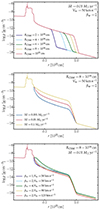 |
Fig. 1. Radial profiles of the mass density used as initial conditions for our radiation-hydrodynamics calculations. From top to bottom, we show groups of models varying in RCSM, Ṁ, and wind velocity profile (i.e., βw and V∞). Radial profiles of the velocity are shown for the last model group in the right panel of Fig. A.4. See Sect. 2.1 and Table 1 for additional information. |
2.1. Initial conditions
Our progenitor model was a 15 M⊙ star on the zero-age main sequence, evolved with MESA (version 10108) at solar metallicity and without rotation. This star reaches core collapse as a red supergiant star with an effective temperature of Teff = 3980 K, a surface bolometric luminosity of L⋆ = 9.6 × 10⁴ L⊙, a surface radius of R⋆ = 652 R⊙, and a surface composition for H, He, C, N, and O given by mass fractions: XH = 0.6987, XHe = 0.287, XC = 1.52 × 10⁻³, XN = 2.28 × 10⁻³, and XO = 5.94 × 10⁻³. The explosion was performed with V1D by depositing 1.47 × 1051 erg within 0.05 M⊙ of a mass cut at 1.65 M⊙ at a constant rate over 0.1 s. When corrected for the envelope binding energy to be shocked, the (asymptotic) total energy is 1.2 × 1051 erg.
This V1D structure (radius, velocity, density, temperature, and composition) was remapped into HERACLES when the shock was within several times 1012 cm below R⋆. This corresponds to a time of 1.04 d since the explosion trigger. Since HERACLES is a Eulerian code, we extended the original V1D grid out to a maximum radius Rmax = 4 × 1015 cm so that we could track for 15 d the evolution of the ejecta as they expand. The HERACLES grid employs 14336 radial grid points, with a constant spacing out to 5 × 1014 cm and a constant spacing in the log beyond. Five tracer particles were used to track the location of the H, He, O, Si, and 56Ni-rich shells but because the preSN model has a massive H-rich envelope, the composition is essentially uniform (and given by that at the surface of the preSN star) in the spectrum formation region at all times studied here.
In this spherical volume between R⋆ and Rmax, we introduced some CSM of diverse properties (Fig. 1). For simplicity, the CSM density corresponds to that of two steady-state wind mass loss rates, chosen in the range 0.001 to 0.1 M⊙ yr−1 within a radius RCSM and 10−6 M⊙ yr−1 beyond – the transition between the two regions occurs over a length scale of a few 1014 cm. This prescribed density was chosen to reflect a phase of high mass loss in the years or decades prior to core collapse and is crafted rather than physically consistent (we make no claim on the physical origin of this mass loss, which is a separate issue). For a given mass loss rate value, Ṁ, the wind density was given by ρ = Ṁ/4πr2V(r); thus, it depends on the velocity profile. In all cases, the wind velocity profile is parameterized by a “hydrostatic”, base velocity, V0, at R⋆, a terminal or asymptotic velocity, V∞, and an exponent, βw controlling the acceleration length scale, such that V(r) = V0 + (V∞ − V0)(1 − R⋆/r)βw. The value of V0 was chosen so that the density connects smoothly at R⋆. Obviously, by assuming a progressive acceleration of the CSM material with radius, the CSM density above R⋆ is much greater than for a prompt acceleration to V∞, by as much as a factor on the order of a thousand.
In Sect. 3, we describe results from radiation-hydrodynamics and radiative-transfer calculations for one model, our reference, which corresponds to a dense CSM with Ṁ = 0.01 M⊙ yr−1, βw = 2, V∞ = 50 km s−1, and RCSM = 8 × 1014 cm. We also explore other models that vary in the extent of the dense CSM (RCSM between 2 × 10¹⁴ and 1015 cm), in mass loss rate (Ṁ of 0.001 and 0.1 M⊙ yr−1), or in the wind velocity profile (βw of 1, 2, and 4; V∞ of 20, 50, 80, and 120 km s−1), as summarized in Table 1. This table also gives the CSM mass, optical depth (assuming an opacity of 0.34 cm2 g−1 representative of an ionized solar-metallicity gas), and the photospheric radius that would result for that same opacity. Prior to shock breakout, this CSM is cold and optically thin to electron scattering (we ignore any presence of dust or molecules in that nearby CSM – it should be promptly destroyed by the SN radiation).
In Fig. 1, the labels give the explicit value for these various model parameters, but in the text we also use a more compact nomenclature. For example, model mdot0p01/rcsm8e14/bw2/vinf5e6 stands for a model whose initial CSM properties correspond to a high mass-loss rate value of 0.01 M⊙ yr−1, RCSM of 8 × 1014 cm, βw = 2, and V∞ = 50 km s−1. When comparing models that differ in only one parameter, we refer to these models through that varying parameter only, omitting parameters that are kept fixed among models in the sample. For example, for those differing in Ṁ only, we refer to models mdot0p001, mdot0p01, and mdot0p1 (see Table 1).
2.2. Radiation hydrodynamics with HERACLES
We performed multi-group radiation-hydrodynamics calculations with HERACLES exactly as discussed in detail and for similar configurations in Dessart et al. (2017). We used eight energy groups spanning from the Lyman to the Balmer continuum. We accounted for bound-free opacity of all species as well as electron scattering (the opacity sources implemented in HERACLES are discussed in Dessart et al. 2015). For simplicity, we ignored the contribution from bound-bound transitions in the HERACLES opacity tables so that the radiative acceleration we obtained in our simulations is an underestimate of the true acceleration, although probably not by much (Chugai et al. 2002). Because the influence of lines is a very complex phenomenon, it is not clear if their simplistic treatment would be a great addition.
2.3. Radiative transfer with CMFGEN
A critical aspect of this work is the post-treatment of the HERACLES simulations with the radiative transfer code CMFGEN. Although this method has been very fruitful for predicting the early-time properties of SN ejecta interacting with CSM, it is not fully physically consistent.
While the simulation in HERACLES is time dependent, the post-treatment with CMFGEN assumes steady state. In practice, we ignored time delays affecting photons emitted from different regions (equivalent to assuming an infinite speed of light) and, in particular, different depths along the line of sight (even though the HERACLES simulation captures the progressive, time dependent, diffusion of radiation, or the heating and the acceleration of the unshocked CSM). The different travel time for these photons arises from the large value of RCSM/c, which may be augmented by the necessary diffusion of these photons across the optically-thick CSM. Photons emitted deeper at earlier times cross an ever changing medium (i.e., in temperature and ionization but also in velocity etc) as they progress along our line of sight. This physical inconsistency is most problematic at the earliest times when the CSM conditions change fast. This includes the rising part of the bolometric light curve, or when one witnesses a rising ionization, as observed during the first day in SN 2024ggi (see, e.g., Jacobson-Galán et al. 2024a; Shrestha et al. 2024; Zhang et al. 2024). The rising ionization implies that light-travel time delays may allow low-ionization lines to persist during a CSM diffusion time (emission lines would first appear blueshifted and progressively become redshifted), although their strength would be considerably reduced relative to lines from higher-ionization lines (e.g., He I relative to He II lines). These light-travel time effects should become secondary when the luminosity and ionization reach a steady state or exhibit a slow evolution.
A second inconsistency arises from using the temperature computed in HERACLES (which assumes LTE for the gas) for the CMFGEN calculation (which solves the nonLTE rate equations). For H-rich compositions where electron scattering and bound-free opacities dominate, this has proven satisfactory. The main benefit from this approach is that this temperature imported from HERACLES reflects the complex radiation hydrodynamics of these interactions, the influence of the shock, the shock breakout signal, the heat- or ionization-wave propagating through the CSM at breakout.
An essential asset of the steady-state radiative transfer calculations with CMFGEN is the direct treatment of the nonmonotonic velocity structure of these interaction configurations. This approach accounts for all emission, absorption, scattering processes occurring in the unshocked ejecta, shocked ejecta, shocked CSM, and unshocked CSM, together with the interplay between the gas and the wavelength- and depth-dependent radiation field. In practice, for each HERACLES snapshot, we select the electron-scattering optical-depth region between 10−4 and ∼50. We sample this region with about 100 points, ensuring a good resolution around the dense shell but also of the unshocked CSM, including the region beyond the photosphere where narrow emission lines form.
Most simulations performed with HERACLES are post-processed with CMFGEN – some are excluded to avoid redundancy (see Table 1). We try to select snapshots that cover from the initial rise of the luminosity out to 15 d after the onset of shock breakout (i.e., when the shock crosses R⋆). We use a uniform composition for the CSM corresponding to the surface composition of the preSN model, and treat all important species including H, He, C, N, O, Mg, Al, Si, S, Ca, Ti, Cr, and Fe. The model atom covers multiple ionization stages to track the ionization stratification of the gas (typically cooler and less ionized further away from the shock). Specifically, we included H I, He I- II, C I- V, N I- V, O I- VI, Mg II- V, Al III- V, Si II- V, S II- V, Ca II- VI, Ti II- IV, Cr II- VI, and Fe II- VII. Because the simulations exhibit different overall ionization depending on the CSM properties or time, some unimportant, low or high ionization stages may be omitted for specific snapshots. In this work, we focus the discussion to optical lines and in particular Hα, but we also touch upon lines of He I, He II, C III, C IV, N III, and N IV as they provide interesting probes of different CSM regions. We discuss how these different lines compare with each other as well as how they evolve in time. Our model set contains information in the ultraviolet and in the infrared for numerous other lines not discussed in this work. This may prove useful for future, high-resolution and high-cadence observations of objects with low or high mass loss rates, and with data in or out of the optical ranges.
The emergent CMFGEN spectra are computed at high resolution, adopting a turbulent velocity of 5–10 km s−1 and a similar frequency-grid spacing. To capture the influence of electron scattering and the associated frequency redistribution, we iterate ten times in order to obtain a converged mean intensity in the formal solution of the radiative transfer equation (for details, see Dessart et al. 2009). With fewer iterations, the wings of most emission lines would be weaker and narrower. Because of the radiative acceleration of the unshocked CSM, the high resolution is essential only at the earliest times – the narrowest emission lines may exhibit a width of 100 km s−1 or more than a few days after the onset of shock breakout.
3. Results for the reference model mdot0p01/rcsm8e14 (aka r1w6b)
3.1. Radiative acceleration of the unshocked CSM
Figure 2 shows some results from the radiation-hydrodynamics calculations for our reference model mdot0p01/rcsm8e14. This model is also known as model r1w6b and was shown to yield a satisfactory match to the multi-band light curves and (low-resolution) spectra of SN 2023ixf (Jacobson-Galán et al. 2023). The top-left panel gives the multiepoch velocity profile versus radius. This evolving structure is generic for such interactions and has been shown multiple times in the past, both for similar HERACLES simulations (see, e.g., Dessart et al. 2015, 2017) or for STELLA simulations (see, e.g., Moriya et al. 2011). The sharp jump in velocity (i.e., the shock) separates the shocked ejecta and CSM from the unshocked CSM. At the start of the simulation, the region below the shock has a complex structure (not shown in detail here) because of the equivalently complicated density structure of the progenitor star (e.g., leading to the formation a reverse and forward shock etc). At shock breakout, about 50% of the total energy is stored in radiation and so only 50% of the explosion energy has been turned into kinetic energy. The region behind the shock is therefore radiation dominated and the escape of that radiation forms the core component of the SN light curve, even in the absence of interaction with CSM. As time goes on, this inner region accelerates and eventually reaches homologous expansion. With the presence of CSM, a reverse shock propagates inwards and decelerates the outer regions of the (already shocked) stellar envelope while a forward shock propagates outwards and crosses the inner regions of the CSM, leading to the formation of a dense shell.
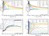 |
Fig. 2. Illustration of radiation and hydrodynamical properties computed by HERACLES for model mdot0p01/rcsm8e14. Top row: Variation in the velocity at multiple epochs versus radius (top left) and versus the distance above the shock (top right). Bottom left: Evolution of the velocity of “mass parcels” initially at radii 0.1, 0.2, 0.35, 0.5, 0.7, 1.0, 1.5, and 3.95 × 1015 cm (the last radius is near the outer grid boundary) and over the full duration of 15 d of the HERACLES simulation. The solid line shows the value of this velocity as read in directly from the simulation. The dashed line shows the same quantity but estimated through a time integral of the radiative acceleration (see the discussion in Sect. 3.1). In all cases, the two curves agree closely until the mass parcel is shocked, which corresponds to the near-vertical jump of the solid lines. The black circles and the stars indicate the velocity at the location where the electron-scattering optical depth is 2/3 (i.e., the photosphere) and at 0.01. Bottom right: Counterpart of the top-left panel but for the luminosity (i.e., quantity Lr = 4πr2Fr). Only the inner half of the grid is shown. |
In this work, we are mostly interested in what takes place beyond the forward shock, thus in the unshocked CSM. Close to the shock, the unshocked material is accelerated to velocities of several 1000 km s−1 and the magnitude of this acceleration drops steeply with radius. At the photosphere (indicated by the filled dots in Fig. 2), the velocity initially rises as it progresses outwards in the CSM because of the photoionization of the CSM caused by the SN radiation (i.e., this reflects the rising velocity with radius of the original CSM), so from 30 to 40 km s−1. This is followed by a strong increase from 40 to 500 km s−1 over the time span of ∼1 to ∼7 d. After shock passage, the photosphere is located in the fast-moving dense shell, with a typical velocity in this model of about 6300 km s−1. In contrast, the outer CSM is modestly accelerated, reaching at 15 d a velocity of 100 km s−1 at 2 × 1015 cm and 62 km s−1 at 4 × 1015 cm, compared to its original velocity of ∼50 km s−1 prior to the SN explosion.
Overall, the acceleration of the unshocked CSM is greatest in optically thick regions below the photosphere, thus, these are largely obscured to a distant observer. An alternate way of showing the acceleration of the unshocked CSM is to plot the multiepoch velocity profile relative to the location of the shock (top-right panel of Fig. 2; this is equivalent to showing the velocity in a frame moving with the shock). We can see more clearly that just ahead of the shock, the acceleration of the unshocked CSM is enormous with velocities rising from a few 10 to a few 1000 km s−1 at 1–2 d, but progressively decreasing at later times to about 300 km s−1 at 15 d.
The bottom-left panel illustrates the physical origin of the acceleration of the unshocked CSM. Here, we show the evolution of the velocity of mass parcels located initially at radii spanning the full extent of the CSM beyond R⋆. Specifically, we place these Lagrangian “tracers” at radii 0.1, 0.2, 0.35, 0.5, 0.7, 1.0, 1.5, and 3.95 × 1015 cm (the last value is just below the outermost grid radius). The solid lines give the results from HERACLES, that is they show the velocity of each mass parcel as it advects. Starting with a mass parcel at (r, t) with a velocity V(r, t), we look for the velocity at t + δt at the new location r + V(r, t)×δt (Zimmerman et al. 2024 show a similar plot based on analytical predictions of the radiative acceleration). The results from HERACLES indicate that the acceleration is indeed huge for the mass parcels located close to the shock and much more modest at large distances, although some acceleration is visible even near the outer grid location. They also show that the acceleration is naturally truncated when the shock reaches the location of a given mass parcel, as evidenced by the sudden jump in velocity (over the 15 d of the simulation, the shock reaches out to a maximum radius of 8.9 × 1014 cm). After being shocked, a mass parcel moves here at about 6300 km s−1.
The dashed lines shown in the bottom-left panel of Fig. 2 correspond to the velocity of the mass parcels estimated from the radiative acceleration computed in HERACLES. Now, starting with a mass parcel at (r, t) with a velocity V(r, t), we compute the new velocity at t + δt and at the new location r + V(r, t)×δt as V(r, t)+gradδt, with the radiative acceleration grad = κesFr/c (κes is the electron scattering opacity, Fr is the radiative flux in the radial direction, and c is the speed of light). Here, both Fr and κes are taken at the relevant location for each (advected) mass parcel and thus reflect the changes in ionization and luminosity with time and depth (see bottom-right panel of Fig. 2). Both solid and dashed curves overlap at most epochs (the curves sharply diverge if and when a given mass parcel is shocked), confirming that the mass parcels are radiatively accelerated, as has been suggested in the past by Fransson et al. (1996) in the context of SN 1993J and by Chugai et al. (2002) in the context of SN 1998S.
The strong radial dependence of the acceleration results from the time and radial evolution of the radiative flux. CSM closer to the shock is influenced by a greater flux (in proportion to r2) but it is also subject to the flux from earlier times because it takes a diffusion time for the radiation to reach the outer, optically thin regions of the CSM. For an optically thin CSM, this time delay would be the free-flight time through the CSM, which is approximately 0.39 R15, CSM d, where R15, CSM = RCSM/1015 cm. For an optically-thick CSM, this delay is augmented by a factor on the order of the electron-scattering optical depth τCSM of the CSM. Hence, a more compact and more optically thin CSM should be more strongly and promptly accelerated, although this radiative acceleration will be eventually limited by the reduced luminosity (i.e., caused by the smaller extraction of kinetic energy from the ejecta). With our model grid of CSM properties, we indeed recover a wide range of CSM acceleration (see Sect. 4).
The question is now to evaluate how this radiative acceleration may be inferred from SN spectra. The formation of the spectrum in these interactions is complex. At large optical depth, both continuum and lines form. If the CSM is sufficiently optically thick, most or all photons arising from the fast-moving ejecta or shock are reprocessed (i.e., absorbed and reemitted) by the CSM. Thus, the photons emitted in this unshocked CSM will scatter multiple times with free electrons before escaping. Upon each scattering, the photons are redistributed in frequency or velocity space. For continuum photons, this produces no obvious signature since their original distribution with wavelength is smooth. For line photons, which are originally emitted over a few Doppler widths (i.e. few km s−1) around the line rest wavelength, this redistribution leads to the transfer of core photons into the wings and the formation of the notorious IIn line morphology with a narrow core and broad symmetric wings. Once a photon is outside of the line core, it is subject to continuum (essentially electron scattering) opacity and thus behaves just like a continuum photon.
Emergent photons located in the narrow cores of emission lines must therefore arise from regions of low electron scattering optical depth, so typically beyond the photosphere (it is by virtue of this property that these narrow line cores should be strongly depolarized; see discussion in Dessart et al. 2024). Because line emission is greater at higher density (particularly true for recombination lines like Hα), these narrow lines will tend to form close to the photosphere. In our calculations, we find that a good proxy for that formation region is where τes is about 0.01–0.1. With time passing, this region may eventually be crossed by the shock so when that occurs, any residual narrow line emission would tend to form just exterior to the shock. In the bottom-left panel of Fig. 2, we indicate with star symbols the evolution of the velocity at that location in our reference model. It shows a very slow rise by 10–20 km s−1 initially as the radiation from shock breakout ionizes and turns the CSM optically thick. There is then a substantial rise up to 400 km s−1 caused by radiative acceleration. Eventually, when the shock reaches the outer CSM, the narrow-line region is limited to just outside the shock and thus probes ever more distant locations where the radiative acceleration has been weaker and thus that velocity should decrease. Eventually, far away from the progenitor surface, the velocity should be the original V∞ of the CSM. Thus, the evolution of the narrow line emission should exhibit a similar pattern, which we discuss in the next section.
3.2. Evolution of individual spectral lines
3.2.1. Evolution of Hα
Figure 3 shows the spectral evolution from 0.83 d until 11.67 d and within 700 km s−1 of the rest wavelength of Hα for our reference model mdot0p01/rcsm8e14 discussed in the preceding section (the full radiative transfer model computed with CMFGEN is not shown since such spectra have been presented and confronted to observations on numerous occasions in the past; see, e.g., a comparison to SN 2023ixf in Jacobson-Galán et al. 2023). The impact of radiative acceleration is immediately visible: the narrow emission line remains bounded within 50 km s−1 (i.e., the original value of V∞) for nearly two days, followed by a considerable broadening until about 10 d, and a hint for a reduction in the extent of the line absorption at the last epoch of 11.67 d, as expected from the discussion in the preceding section. For clarity, we add a vertical bar indicating the velocity at τes of 0.01 and indicated by star symbols in the bottom-left panel of Fig. 2.
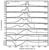 |
Fig. 3. Evolution of the spectral region centered on the rest wavelength of Hα for model mdot0p01/rcsm8e14. The symmetric solid vertical lines on each side of the origin correspond to the velocity at the location in the unshocked CSM where the electron-scattering optical depth is 0.01, thus exterior to the location of the photosphere. The dashed vertical lines correspond to ± V∞ of the original, unadulterated CSM. The spectral evolution in other H I Balmer lines is analogous to that shown here for Hα (see the case of Hβ shown in the left panel of Fig. A.2). Note that He II 6560.09 Å contributes some flux on the blue edge of Hα, well separated from it initially but overlapping with the Hα emission at 2–5 d. The ordinate range changes in each panel for better visibility. |
The results shown in Fig. 3 are, however, a little more complex than what we would have anticipated. First, there is a He II transition on the blue side of Hα at 6560.09 Å. This emission starts weak, strengthens as the temperature of the CSM rises in the initial few days and then disappears around 5 d as the conditions become too cool for He II emission. It is also impacted by the radiative acceleration of the CSM so He II 6560.09 Å progressively broadens until it disappears. Because of this broadening, the contribution from He II 6560.09 Å and Hα overlap at 2–5 d and the “contaminant” is not easily identified.
A second aspect is that Hα starts roughly symmetric but becomes progressively blueshifted in both absorption and emission. At 0.83 d, the Hα line is well centered on the rest wavelength, with roughly symmetric emission blueward and redward, but it exhibits excess emission on the blueside beyond 50 km s−1. All the CSM beyond 2 × 1014 cm moves at 40–50 km s−1 at that time (see bottom left panel of Fig. 2), so this likely arises from the escape into the line wings of photons trapped in the highly optically thick line core. This feature affects all optically-thick lines and is visible too here in He II 6560.09 Å. After 5 d, the “narrow” Hα line has a blueward extent out to about 400 km s−1 with a clear P-Cygni profile morphology. Unlike stellar winds that increase in velocity from the hydrostatic base to their asymptotic velocity, the P-Cygni trough here probes the region at ∼ 500 km s−1 just outside the photosphere (blue edge of the trough) out to the slow moving outer CSM with velocity of ∼ 100 km s−1. In this model, this P-Cygni trough disappears at later times because the CSM density is too low (see alternate results for model mdot0p01/rcsm1e15 for the case where the CSM is even more extended).
The fact that most of the changes in emission and absorption are seen blueward of the rest wavelength of Hα is a consequence of optical depth effects. Regions near the mid-plane or from the receding hemisphere suffer greater absorption. For optically thin conditions, the line would exhibit a symmetric emission relative to the rest wavelength and no absorption. Optical-depth effects here may be exacerbated by the assumption of spherical symmetry and steady-state constant velocity at large distances (there could for example be more turbulence, or some nonmonotonicity of the flow at large distances etc).
3.2.2. Evolution of other lines
Figures 4–8 show the evolution for other lines in the reference model mdot0p01/rcsm8e14, namely He I 5875.66 Å (Fig. 4), He II 4685.70 Å (Fig. 5), C IV 5801.31 Å (Fig. 6), N IV 7122.98 Å (Fig. 7), and C III 5695.92 Å (Fig. 8). There is some redundancy in line evolution. For example, Balmer lines tend to show a similar evolution so we show the evolution for Hβ in the left panel of Fig. A.2 but skip the discussion of additional H I transitions. The same applies to He II lines so we show only the evolution of He II 5411.52 Å in the right panel of Fig. A.2.
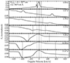 |
Fig. 4. Same as Fig. 3, but for He I 5875.66 Å. This line is present at early times until about 1 d and then again after ∼3 d, but absent between, when the ionization of the unshocked CSM is too high. |
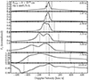 |
Fig. 5. Same as Fig. 3, but for He II 4685.70 Å. This line is essentially unblended and present until ∼5 d, after which the He ionization is too low. The symmetric solid vertical lines on each side of the origin correspond here to the velocity at the location in the unshocked CSM where the electron-scattering optical depth is 0.1. |
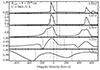 |
Fig. 6. Same as Fig. 3, but for C IV 5801.31 Å. Here, the solid vertical bars on each side of the origin correspond to the velocity at the location in the unshocked CSM where the electron-scattering optical depth is 0.1. |
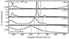 |
Fig. 7. Same as Fig. 3, but for N IV 7122.98 Å. This line is absent prior to ∼1 d and after ∼5 d, because of the unsuitable ionization state of the unshocked CSM at those epochs. This spectral region contains other N IV lines at 7109.35, 7111.28, and 7127.25 Å. Here, the solid vertical bars on each side of the origin correspond to the velocity at the location in the unshocked CSM where the electron-scattering optical depth is 0.1. |
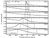 |
Fig. 8. Same as Fig. 3, but for C III 5695.92 Å. Besides the evolution of that line in width caused by the radiative acceleration of the unshocked CSM, its strength also varies in time with a minimum around 1.5 d caused by the high ionization of the unshocked CSM (at those epochs, C IV is the dominant ion). |
The narrow component of the He I 5875.66 Å emission line (Fig. 4) shows at 0.83 d a similar profile to Hα, roughly symmetric in emission around the rest wavelength (with a width reflecting a formation within the accelerating part of the original, unadulterated wind CSM) and with an excess emission in the blue related to photon escape in the line wings. In the first spectrum, we clearly see a P-Cygni trough (there is a marked absorption at about −40 km s−1). As the CSM is progressively photoionized during shock breakout, He becomes predominantly He+ and He I lines disappear, before reappearing again after 3 d when the CSM cools and recombines. During this second phase, He I 5875.66 Å exhibits a P-Cygni profile morphology, with a strong absorption extending to about −450 km s−1 at 10 d and little emission on the blue side. As for Hα, the relatively narrow emission falling within ± 100 km s−1 at 11.67 d forms in the distant CSM whereas the extended trough forms much closer in, just outside of the shock. In other words, the P-Cygni profile forms in a region with a radially declining velocity.
The He II lines show a reverse trend relative to He I lines since they take some time to strengthen as the CSM heats up but survive only as long the CSM stays sufficiently hot. Indeed, the narrow component of the He II 4685.70 Å line emission progressively strengthens up until 3–5 d before decreasing and vanishing at about 7 d (Fig. 5). The emission has a similar shape as Hα at 0.83 d but with a marked blueshift. Radiative acceleration becomes visible after about 2 d when the line stretches out to 150 km s−1 blueward of the rest wavelength (the red side of the profile remains narrow and hardly changes). At 7–10 d, the model predicts a residual blueshifted absorption out to −500 km s−1 but it is extremely weak (slight inflection at the percent level).
Figure 6 shows the spectral region within ± 700 km s−1 of the rest wavelength of C IV 5801.31 Å. As for He II 4685.70 Å, this line disappears quickly after 5 d because of the reduction in ionization of the unshocked CSM. There is no C IV 5801.31 Å emission or absorption from the more distant, cooler, CSM so a narrow component is only present at the earliest times in the model. This C IV transition is a doublet, whose other component at 5811.97 Å is visible at right as a close replication of C IV 5801.31 Å. Unlike the lines previously discussed, this C IV line is strongly blueshifted at all times but this is striking at the earliest epochs (prior to ∼2 d) when the line is narrow. This occurs because the line tends to form closer to the photosphere where occultation (or optical-depth) effects are greater. After 2 d, the line blue edge broadens and eventually forms a P-Cygni absorption trough extending to several 100 km s−1. Unlike Hα or He I 5875.66 Å, this doublet C IV transition does not exhibit an absorption at early times, which may arise from the fact that the line forms over a restricted range of depths (i.e., where the optical depth is low but the density still high enough and importantly where the temperature is high enough).
Figures 7–8 show the evolution for N IV 7122.98 Å and C III 5695.92 Å. Both exhibit a similar behavior with strongly blueshifted emission at all times (due to optical-depth effects), a lack of P-Cygni absorption (due the relatively confined formation region of these lines). The relatively high ionization of these lines limits their presence to early times with a very modest strength at the earliest times when the CSM is still heating up and rising in ionization.
To summarize, the narrow component of the emission lines discussed above shows both the influence of radiative acceleration and ionization, with line widths starting narrow and corresponding to the unadulterated CSM velocity but growing with time to reach about 500 km s−1. For low ionization lines still present at 10 d, their narrow component starts showing signs of a reduction in velocity as the more distant CSM is being probed. Optical-depth effects tend to quench the emission from the receding part of the CSM, causing a blueshift of the line emission. This skewness is greater for lines of high ionization because they tend to form over a smaller volume and close to the photosphere. Although the lines are skewed, the line emission remains immediately adjacent to the rest wavelength. None of our model profiles show the detached narrow emission reported by Pessi et al. (2024) for most lines observed in SN 2024ggi – this offset may be due to adopting an inadequate recession velocity to the SN. Finally, to facilitate the comparison of all lines at once, we present a mosaic of numerous lines but all at 1 d after the onset of shock breakout in the reference model mdot0p01/rcsm8e14 in Fig. A.3.
4. Dependences on CSM velocity, density, and extent
Having presented in detail the reference model mdot0p01/rcsm8e14 in terms of radiation-hydrodynamics properties (shock propagation, radiative acceleration of the unshocked CSM etc) and the associated characteristics of narrow emission lines versus time, we go on to explore the sensitivity of these results to variations in CSM properties. We start in the next section by addressing the impact of the extent of the CSM, followed by the impact of the CSM density (Sect. 4.2), and, finally, the impact of the CSM velocity profile (Sect. 4.3).
4.1. Impact of CSM extent
In this section, we discuss the change in the results discussed earlier when the CSM extent was varied while other CSM characteristics were kept the same. Specifically, we study models with a CSM mass loss rate of 0.01 M⊙ yr−1 and wind velocity parameters of βw = 2 and V∞ = 50 km s−1, but the value of RCSM is increased from 2 × 1014 cm to 1015 cm. Here, these models are named rcsm2e14, rcsm4e14, rcsm6e14, rcsm8e14, and rcsm1e15.
Figure 9 shows some results from the radiation-hydrodynamics calculations for this model grid. With increasing RCSM, the CSM optical depth increases (although the bulk of the optical depth arises from the inner CSM, which is the same in all five models) and the photosphere is located further out at 1.7, 3.1, 4.1, 5.7, and 7.1 × 1014 cm in the models rcsm2e14 to rcsm1e15. The diffusion time through the CSM is longer so the light curve rise time to maximum is greater for more extended CSM. Relative to a time of first detection at the outer grid boundary set to 1041 erg s−1, the rise time increases from ∼1.5 d (and a peak Lbol in excess of 1044 erg s−1) in model rcsm2e14 up to ∼2.5 d (and a peak Lbol of 5 × 1043 erg s−1). The time-integrated bolometric luminosity over the first 15 d varies from around 1.4 to 3 × 1049 erg in this model set. In model rcsm1e15, the shock is still embedded in the dense CSM at the end of the simulation and the luminosity is still very large.
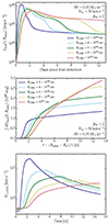 |
Fig. 9. Results from the radiation-hydrodynamics calculations for models differing in RCSM. Top: Bolometric luminosity recorded at the outer boundary and starting when the power exceeds 1041 erg s−1. Middle: Same as top for the cumulative bolometric luminosity. Here, we use the HERACLES time modified for the light-travel time to the outer boundary. Bottom: Evolution of the velocity at the location in the unshocked CSM where the electron-scattering optical depth is 0.01. When that location is shocked, we report the velocity at the radius immediately exterior to the shock. |
The evolution of the velocity at the location where the unshocked CSM optical depth is 0.01 is shown in the bottom panel of Fig. 9 – this is a good representation of the Doppler-velocity width of the narrow emission line component (see the previous section). The greatest velocity is obtained in model rcsm2e14 with a peak at 2100 km s−1 at only 2.5 d after the start of the simulation. This occurs despite the relatively low luminosity (and its time integral) of that model. In contrast, the smallest velocity is obtained for the rcsm1e15 model with a velocity of 320 km s−1 attained just before the end of the simulation at 14.5 d, and thus in spite of the much larger luminosity (and time integral). Models with intermediate values of RCSM yield values that lie in between these two models.
We thus obtain the paradoxical result that the greater the CSM mass and extent, the lower the recorded acceleration. This arises simply from the fact that for a more extended CSM, the region where the narrow emission line component forms is located further away from the deeply embedded shock or ejecta regions where the radiation decouples from the gas. Beyond that location, the luminosity is essentially constant, so the flux drops as 1/r2, and the associated radiative acceleration is considerably weaker at greater distances. Paradoxically, the radiative acceleration to be recorded from narrow emission lines would be greater for more compact CSM although that observable acceleration would be short-lived because of the imminent shock passage.
We post-processed these simulations with CMFGEN, covering all epochs from a fraction of a day until the end of the simulations at 15 d. Figures 10–12 show the evolution at a few, distinctive epochs in the evolution of Hα within ±700 km s−1 from the rest wavelength for models rcsm2e14, rcsm6e14, and rcsm1e15 (in the appendix we also show results for the intermediate model rcsm4e14 in Fig. A.4 – corresponding results for model rcsm8e14 are presented in Sect. 3.2).
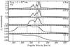 |
Fig. 10. Evolution of the spectral region centered on the rest wavelength of Hα for model mdot0p01/rcsm2e14. The symmetric solid vertical lines on each side of the origin correspond to the velocity at the location in the unshocked CSM where the electron-scattering optical depth is 0.01. The dashed vertical lines correspond to ±V∞, where V∞ is the terminal wind velocity of the original, unadulterated CSM. |
The drastic differences are immediately apparent. For model rcsm2e14, the Hα profile is still narrow at 0.5 d but broadens considerably within 0.5 d and the profile extends beyond the plot limits at 1.17 d. The Hα profile emission is strongly blueshifted with essentially no flux redward of the rest wavelength although some emission is present at the rest wavelength. In model rcsm6e14, the broadening and blueshift of the line emission start at ∼ 2 d, reaching some plateau at about 4 d; afterward, a weakening P-Cygni profile forms with a trough peaking at about −500 km s−1, which is the value of Vτ = 0.01 at about 5 d. In model rcsm1e15, the evolution is much reduced. The Hα profile stays narrow for up to about 2.5 d, after which a slow broadening appears leading to a maximum blueshift of the emission and absorption out to about 300 km s−1, again in agreement with Vτ = 0.01.
In all profile simulations, the narrow-line emission extends to large velocities on the blue side, up to values well in excess of the velocity at optical depth 0.01. This arises because there is no sharp boundary separating the narrow line emission from the region below the photosphere from where line emission appears both broader (the material is more strongly radiatively accelerated, and eventually shocked) and influenced by electron scattering (thus broadened because of the scattering with relatively high-velocity, thermal electrons).
4.2. Impact of CSM density
In this section, we study the impact of the CSM density on the radiative acceleration of the unshocked CSM as well as the spectral signatures for the narrow emission line component. These results are analogous to those obtained in the previous section for variations in RCSM. Specifically, we considered model counterparts to the reference model in which the mass loss rate of 0.01 M⊙ yr−1 is raised to 0.1 or reduced to 0.001 M⊙ yr−1. All other model parameters were kept identical, namely, βw = 2, V∞ = 50 km s−1, and RCSM = 8× 1014 cm. We refer to these models as mdot0p001, mdot0p01, and mdot0p1.
Figure 13 shows the evolution of Lbol, its time integral, and Vτ = 0.01 for this model set. The factor of a hundred in mass loss rate implies a similar factor in CSM optical depth, which affects the location of the photosphere (at 3, 5.5, and 6.5 × 1014 cm) although not by as much as in the preceding section because the extent of the dense CSM is the same in all three models (with a dramatic drop in CSM density at 8 × 1014 cm). The extraction of kinetic energy from the CSM is modest in model mdot0p001 (∼1.2 × 1049 erg) but large in model mdot0p1 (∼8 × 1049 erg).
The combination of a relatively low extraction of kinetic energy and the relative large radius of formation of the narrow-line emission region leads to a modest Vτ = 0.01 of at most ∼240 km s−1 in model mdop0p001. For enhanced mass loss rate, Vτ = 0.01 reaches about 500 km s−1 in model mdot0p01, and 1200 km s−1 in model mdot0p1 (continuing that model mdot0p1 to later times would have yielded even higher velocities).
Figure 14 shows the evolution of the Hα region for model mdot0p001 (bounds are ±700 km s−1) and for model mdot0p1 (bounds are ±2000 km s−1). In model mdot0p001, the influence of the radiative acceleration on Hα is well identified, with a small and progressive broadening of the line after a fraction of a day, and the development of a nearly symmetric and well defined P-Cygni profile. This lack of blueshift here is caused by the relatively low optical depth of the CSM, which affects little the distant, and in some sense detached regions where the narrow emission line component forms. The line also clearly exhibits the progressive broadening and subsequent narrowing at late times, as obtained in all model curves of Vτ = 0.01. Not surprisingly, the radiative acceleration in the model with high mass loss rate is considerably reduced. Model mdot0p1 shows the first signatures of Hα broadening after 7 d and this continues until the latest epoch at 15 d when the line exhibits a P-Cygni profile with a maximum absorption in the trough at about 1300 km s−1. The narrow line emission exhibits a strong blueshift at all times because the CSM is now highly optically thick, causing a strong occultation effect of the mid-plane regions and those receding from the observer.
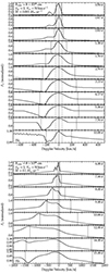 |
Fig. 14. Same as Fig. 10, but for models differing in Ṁ, covering from low (top panel) to high mass loss rates (bottom panel). |
4.3. Impact of a wind velocity law
In this final exploration, we consider CSM configurations that differ in terms of the wind velocity profile. All models use a mass loss rate of 0.01 M⊙ yr−1 and a value of 8 × 1014 cm for RCSM for the high density CSM, but the wind velocity covers values of 1, 2, and 4 for βw and 20, 50, 80, and 120 km s−1 for the original CSM velocity. Because the CSM density varies as Ṁ/r2V, the different radial variation in the velocity imply different density profiles (even for the same Ṁ). Consequently, the bolometric light curves shown in Fig. 15 (top panel) differ between models. In particular, winds with a long acceleration length scale (high values of βw) or low terminal velocities initially (low V∞) correspond to a CSM with a larger density, greater diffusion time, greater extraction of kinetic energy, and thus produce light curves with a longer rise time, possibly with a greater peak luminosity (but not necessarily), and a greater time-integrated bolometric luminosity.
The results for Vτ = 0.01 are different for every model. In all cases, Vτ = 0.01 initially indicates roughly the original value of V∞, typically reduced by a few tens of percent because this region is located in the accelerating part of the original, unadulterated wind. The value of Vτ = 0.01 rises earlier in models with more tenuous CSM (high V∞ or low βw). It reaches a large maximum value in models with a denser CSM, although that maximum is reached later – the range of peak values covers roughly 400 to 700 km s−1 at 10 to 14 d after the start of the simulation.
Figure 16 shows the results for two specific cases differing in the value of V∞, taking the extremes at 20 and 120 km s−1 (βw is two in both cases). For a V∞ of 20 km s−1, we were able to converge one model at very early times when the SN radiation has hardly crossed the CSM at all (the SN luminosity is only 1% of that at peak). At 0.83 d, the model predicts a strongly blueshifted narrow Hα component with a P-Cygni trough that extends to about −50 km s−1. We suspect this is due to photon leakage in the wings of Hα where the line optical depth is lower. The line then changes in morphology as the CSM heats up but it remains relatively narrow until about 3 d, after which the broadening starts in earnest and peaks at ∼10 d with a value of ∼600 km s−1.
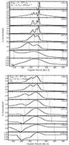 |
Fig. 16. Same as Fig. 10, but for two models differing in the original CSM velocity V∞ with a value of 20 km s−1 (top panel) and 120 km s−1 (bottom panel). |
In the model with a larger initial value of V∞ of 120 km s−1, the narrow Hα emission component starts broader and the broadening due to radiative acceleration kicks in already at 1.5 d. The broadening is strongest in the blue part of the line and extends out to about 400 km s−1 with a clear P-Cygni profile morphology at late times. This P-Cygni profile forms despite the decreasing velocity with radius: The central, narrow emission comes from the outer CSM regions whereas the extended blue absorption arises from deeper regions located nearer the photosphere.
Inferring the original velocity of the CSM from the emergent spectrum is difficult because the CSM is radiatively accelerated immediately at shock breakout. The radiation from the embedded shock accelerates the CSM as it streams away from the shock and diffuses through the CSM. Thus, this radiative acceleration is intimately tied to the rising luminosity from the SN. Unless the SN is discovered at the earliest times when its luminosity is still very low, the CSM probed by high-resolution spectra will already be affected by radiative acceleration.
Because of the radiative acceleration of the CSM, the need for the highest spectral resolution is necessary only at the earliest times. Once the narrow emission line component has broadened, the main limiting factor may instead be the signal-to-noise ratio. The exception is for configurations in which distant CSM is still optically-thick in some lines like Hα and produce a persisting, narrow (albeit likely weak) P-Cygni profile (see, e.g., the case of SN 2020pni; Terreran et al. 2022).
5. Broad- versus narrow-line emission evolution
The information contained in high-resolution spectra is complementary to that present in low-resolution spectra. Any information in high-resolution spectra and over a broad wavelength range should match that present in low-resolution spectra. This is a critical check that no erroneous normalization of high-resolution spectra has been done. With high resolution, we capture the narrowest line features, and because they are obtained with echelle spectra, broad lines that lie over multiple orders are compromised. Thus, high-resolution spectra are mostly useful to constrain the distant CSM where line broadening effects due to radiative acceleration and electron scattering are reduced. In contrast, low- or medium-resolution spectra provide critical information on the regions closer to the photosphere, where line broadening by electron scattering, by radiative acceleration, and eventually by the fast expansion of the shocked material are large. Hence, a combination of low-, medium-, and high-resolution, high-cadence observations is needed to build a complete picture of SN explosions. Such data are available at best for a few objects only.
Figure 17 illustrates the combined evolution of the narrow and broad emission (and absorption) components of Hα for models rcsm2e14 and rcsm8e14, which differ in the value of RCSM (the other model parameters for both are Ṁ = 0.01 M⊙ yr−1, βw = 2, and V∞ = 50 km s−1). In both models, the early phase during which the narrowest line emission component is seen is also the phase during which the broad component exhibits strong electron-scattering broadened wings extending out to 2000–3000 km s−1 from line center. In model rcsm2e14, the wings weaken quickly and the broadened narrow component persists until about 2 d. By 2.5 d, the entire Hα profile is in absorption, with multiple components reflecting absorption from the unshocked CSM around the photosphere and from the fast-moving dense shell. The spectrum then becomes quasi featureless when the entire CSM has been swept up inside the dense shell and a weak Hα absorption appears at about −7500 km s−1.
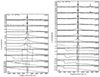 |
Fig. 17. Evolution of the broad and narrow emission components in the Hα spectral region from ∼0.5 d until ∼15 d after shock breakout for model rcsm2e14 (left) and rcsm8e14 (right). The symmetric solid vertical lines on each side of the origin correspond to the velocity at the location in the unshocked CSM where the electron-scattering optical depth is 0.01. For the CDS velocity of ∼6000 km s−1 in the rcsm8e14 model, the He I 6678 Å trough extends out to the Hα rest wavelength and thus may overlap with a narrow Hα component. |
In model rcsm8e14, the evolution is comparable but the electron-scattering broadened wings survive until about 5 d. During the next 5 d, the photosphere is in the fast-moving dense shell and one sees a strong broad blueshifted absorption with a maximum absorption at about −6000 km s−1 (this is the velocity of the dense shell). However, a narrow P-Cygni profile persists in this case until about 13 d and suggestive of a residual unshocked CSM at large distances but relatively broadened due to radiative acceleration. By 15 d, the narrow component has vanished.
6. Discussion and conclusions
In this paper, we present radiation-hydrodynamics simulations of red supergiant stars exploding within some CSM characterized by a different extent (i.e., RCSM), different density (i.e., Ṁ), and different velocity profile (βw and V∞ parameters). For many of these interaction configurations (five with different values of RCSM; three with different Ṁ; three with different V∞), we computed nonlocal thermodynamic equilibrium (NLTE) radiative-transfer simulations at multiple epochs covering from the onset of shock breakout until the “ejecta” phase when the CSM has been fully swept-up by the shock and when the spectrum forms primarily within the ejecta. By combining radiation hydrodynamics and detailed radiative transfer, we can document how the dynamical properties of the ejecta and CSM translate into spectral properties both for the broad and the narrow line components. Indeed, at all times, our synthetic spectra reveal emission and absorption from distinct regions, potentially including the unshocked CSM, the shocked CSM, the shocked ejecta, and the unshocked ejecta. Each region has a distinct velocity, temperature, and density and thus leaves a specific imprint on spectra. The subject of this study was to document such properties with a particular emphasis on the information contained on the smallest velocity scale and revealed in high-resolution spectra. The main limitations of this work are the assumption of steady-state, spherical symmetry, and the neglect of line opacity, although we surmise that these are secondary relative to the importance of radiative acceleration and optical-depth effects.
In all simulations, we find that the unshocked CSM undergoes significant radiative acceleration prior to being shocked, as has been proposed in the past (Fransson et al. 1996; Chugai et al. 2002; Dessart et al. 2015; Tsuna et al. 2023). This acceleration starts at the onset of shock breakout and essentially persists for as long as there is SN radiation. However, this acceleration is strongest when the SN luminosity is large and thus primarily during the early photospheric phase. The acceleration is caused by momentum transfer from radiation to the gas and scales with the flux (i.e., not the luminosity). The radiative acceleration is therefore maximum near the shock and declines as 1/r2 with increasing distance above the shock. Because the agent leading to radiative acceleration is the SN radiation, the original CSM velocity is altered immediately at the onset of shock breakout – our ability to infer the original CSM velocity is thus strictly impossible since it would require obtaining high-resolution spectra of the exploding star before shock breakout (i.e., before the SN had even been discovered). The best that can be done is to obtain high-resolution spectra at the earliest epochs after shock breakout, when the SN luminosity is still modestly greater than the progenitor luminosity (and the earlier the better).
We also find that the radiative acceleration can give rise to very large velocities of the unshocked CSM, with maximum values of several 1000 km s−1 and thus barely below the velocity of the shocked material (which is no less than about 5000 km s−1, whatever the CSM mass and extent). Such a strong radiative acceleration just ahead of the shock weakens the shock and is a strong limitation for X-ray emission at early times after shock breakout. In fact, the actual shock power is much weaker than the SN luminosity leaking from behind the shock at those early times and could explain the low X-ray luminosities observed in SNe II-P interacting with CSM at early times. Overall, the shock appears strong once it has cleared out of the dense CSM indicated by RCSM in our simulations.
In interacting SNe, the narrow emission line component arises from regions external to the photosphere. Indeed, at and below the photosphere (where the radiative acceleration is greater), the frequency redistribution caused by electron scattering is an important line broadening mechanism, depleting line core photons and boosting emission line wings. In contrast, beyond the photosphere, the electron-scattering optical depth is small and the main line broadening mechanism is Doppler broadening, which thus reflects the relatively low expansion velocities of the distant, unshocked CSM. A good proxy for this region is where τes = 0.01 and we thus refer to this velocity as Vτ = 0.01.
With our large grid of simulations, we find that the radiative acceleration of such a distant CSM (where narrow line emission forms) leads to radial velocities that exhibit a bell-shaped morphology. Initially, the velocity rises as the CSM becomes ionized by the SN radiation (i.e., Vτ = 0.01 rises to esentially V∞). As more flux reaches those outer regions, Vτ = 0.01 slowly rises to a few hundred km s−1 in cases of extended or dense CSM or rapidly rises to several thousand km s−1 in cases of compact or tenuous CSM. The main reason for this difference is the scaling of the radiative acceleration with the flux, which is maximum for configurations in which the region with τ = 0.01 is close to the shock. This is paradoxical since it indicates that the radiative acceleration to be observed from high-resolution spectra will be maximum in SNe II with less CSM. In contrast, strong interactions will show much reduced acceleration because the regions with τ = 0.01 are at large distances, where the radiative flux is strongly diluted.
By post-processing our radiation-hydrodynamics calculations with detailed NLTE radiative-transfer calculations, we can go beyond speculations and confirm the previous findings. Using a reference model with 0.01 M⊙ yr−1, RCSM = 8 × 1014 cm, βw = 2, and V∞ = 50 km s−1, we documented the evolution of the narrow line component of H I, He I, He II, C III, C IV, and N IV lines in the optical. Their behavior mirrors what is obtained for the broad component in terms of overall strength because of the similar evolution in ionization of the optically thick and optically thin regions lying interior and exterior of the photosphere. For example, He I lines are strong initially, weaken as the CSM ionization increases after shock breakout, are eventually reborn after shock passage and further cooling of the spectrum formation region, and ultimately disappear as recombination kicks in. Lines of He II or C IV have similarly very limited survival times since they require a higher ionization or temperature that is fundamentally short lived.
In all cases, we find that the narrow emission line component is strongly impacted by radiative acceleration. These narrow spectral features are therefore very sensitive probes of the unshocked CSM. We find that they reflect closely the evolution of Vτ = 0.01 reported above. The original, narrowest emission lines are present only at the earliest times, with broadening of the line emission as the SN luminosity ramps up. The lines can become significantly broad and no longer require the highest resolution in order to be revealed. They probe CSM velocities of several 100 km s−1 and may thus be resolved even with a standard spectral resolution. The signal-to-noise ratio may instead be a stronger requirement since the broadened lines may be weak relative to the underlying broad, electron-scattering broadened emission. Similarly, inadequate setting of the “continuum” emission level may also lead to an inadequate interpretation of the broadening of the narrow emission line component. This issue may impact data obtained with echelle spectra.
A second property is the blueshift of narrow emission features. This blueshift may be small early on in lines forming over a relatively extended volume of the CSM like Hα. Lines of higher ionization like C IV 5801.31 Å or N IV 7122.98 Å show a strong blueshift, which results from their formation close to the photosphere where the temperature and ionization are higher. Consequently, they are more strongly affected by optical-depth effects. As the unshocked CSM becomes ionized, optically-thick, and radiatively accelerated, the blueshift increases and the bulk of the “narrow” line emission occurs blueward of the rest wavelength.
A narrow-line emission may be present until late times if the distant CSM is dense enough. In our simulations, we adopted a low outer CSM mass loss rate of 10−6 M⊙ yr−1 so that a narrow emission component is essentially lacking at the end of our simulations at 15 d (except in our models with the highest mass loss rate of 0.1 M⊙ yr−1 or extent of 1015 cm). Such a detection of a narrow Hα line up until a month after explosion was made for SN 1998S by Fassia et al. (2001) and revealed an absorption at ∼ 50 km s−1 from the rest wavelength not just of Hα but of multiple H I and He I lines. It suggests a gradual decline of the CSM density, perhaps with mass loss rates of 10−4 M⊙ yr−1 at large distances, as well as an original CSM velocity probably close to 50 km s−1 since this distant material should experience very modest radiative acceleration. We leave the modeling of this more distant material to a future work.
Our simulations indicate that radiative acceleration of the unshocked CSM may lead to velocities as high as several 1000 km s−1. Such values remain smaller than the post-shock velocities, which (in our standard explosion model) are systematically greater than 5000 km s−1 (in the absence of CSM these velocities reach about 10 000 km s−1). This indicates that the so-called “intermediate-width” emission component at around 1000 km s−1 cannot be associated with post-shock gas. Therefore, it is emission from unshocked CSM that has either been radiatively accelerated or electron-scattering broadened.
In our forward-modeling approach, we used one red supergiant progenitor model with a standard surface radius and varied the CSM properties. We kept the values of RCSM below 1015 cm since the focus was not on the rare superluminous interacting SNe (e.g., SN 2010jl), but instead on the Type II SNe that are more routinely observed to exhibit short-lived signatures of interaction with CSM (Bruch et al. 2021, 2023; Jacobson-Galán et al. 2024b). Our CSM radii are thus sizably smaller than those inferred, for example, in Boian & Groh (2020, whose sample counts numerous superluminous interacting SNe). Caution is, however, required when comparing radii between different studies. The parameter Rin used in Boian & Groh (2020) defines the radius where the diffusive, inner boundary flux is injected at the time considered; thus, does not correspond to R⋆. It is instead some time-evolving radius within the unshocked CSM, on the order of Rphot, and thus external to the shock. In the present work, we also artificially introduce a kink in the density distribution at RCSM that corresponds to the outer edge of the dense CSM (adopting a kink is convenient and also facilitates the interpretation of model results since it leaves a clear mark in the spectral evolution). Obviously, the CSM mass loss rate must drop at large distances but it may do so at different rates, either precipitously or continuously (or with other trends; see, e.g., the inferences for SN 2023ixf; Bostroem et al. 2024; Nayana et al. 2024). As demonstrated in this work, a similar caution is required when interpreting CSM velocities (which impact the CSM density for a given mass loss rate or impact the mass loss rate for a given CSM optical depth) since they are affected by radiative acceleration.
At present, there are limited high-resolution data available, which our simulations can be compared to. High-resolution spectra of SN 1998S at early times (Leonard et al. 2000; Fassia et al. 2001) are comparable with our models with extended, dense CSM-like models, such as mdot0p1 or rcsm1e15. The high-resolution observations of SN 2024ggi at about 1–1.5 d after explosion reported by Pessi et al. (2024) and Shrestha et al. (2024) are in good agreement with our model rcsm4e14 and serve as analogs in terms of the narrow line evolution and blueshift. Unfortunately, these observations do not cover until later times. The adopted SN redshift by Pessi et al. (2024) suggests a complete offset of all lines relative to their rest wavelength by about 70 km s−1, which is in conflict with our model predictions. We note that models do predict emission line blueshifts, but with emission present at the rest wavelength and little emission redward of the rest wavelength. The observations of SN 2023ixf reported by Smith et al. (2023; see also Zimmerman et al. 2024) do show similar patterns with a progressive broadening of the Hα emission over the first two weeks in a similar fashion to what is obtained here. There is also a clear narrow emission that persists at later times, as reported for SN 2023ixf (see, e.g., Fig. 4 in Jacobson-Galán et al. 2023) or for SN 2024ggi (Jacobson-Galán et al. 2024a; Zhang et al. 2024). A detailed confrontation of the simulations presented in this work to observed high-resolution spectra of SNe II with interaction is deferred to a forthcoming study.
Overall, SN 2020pni probably offers the most complete spectral evolution of narrow emission line components (Terreran et al. 2022), reflecting that obtained in the present simulations. Specifically, this is a narrow component broadening with time for a few days, then becoming narrower at later times, as the narrow-line formation region shifts to more distant locations (where radiative acceleration is much weaker). This bell-shaped morphology of the width of narrow-line emission (with possible absorption) is a fundamental signature of radiative acceleration in extended dense CSM surrounding exploding RSG stars.
The SN shock breakout corresponds to the emergence of the shock from the optically thick, dense envelope of the star. This phenomenon is associated with the progressive release and escape of radiation trapped behind the shock. It corresponds to a short-lived phenomenon, well-defined in time, in red supergiant stars without CSM (i.e., duration of a fraction of an hour; see, e.g., Gezari et al. 2008) or in blue-supergiant stars (i.e., duration of minutes; see, e.g., the case of SN 1987A; Ensman & Burrows 1992). However, in the presence of an optically thick CSM, this burst of radiation is smeared in time by diffusion. It also becomes difficult to disentangle from the continuous supply of interaction power as the shock crosses this CSM. This phase can then extend over hours, days, and even weeks for a very extended dense CSM.
All simulations in this work are available at https://zenodo.org/communities/snrt.
Acknowledgments
LD thanks Wynn Jacobson-Galán for fruitful discussions. This work was supported by the “Programme National Hautes Energies” of CNRS/INSU co-funded by CEA and CNES. This work was granted access to the HPC resources of TGCC under the allocation 2023 – A0150410554 on Irene-Rome made by GENCI, France. This research was supported by the Munich Institute for Astro-, Particle and BioPhysics (MIAPbP) which is funded by the Deutsche Forschungsgemeinschaft (DFG, German Research Foundation) under Germany’s Excellence Strategy – EXC-2094 – 390783311. This research has made use of NASA’s Astrophysics Data System Bibliographic Services.
References
- Boian, I., & Groh, J. H. 2020, MNRAS, 496, 1325 [CrossRef] [Google Scholar]
- Bostroem, K. A., Sand, D. J., Dessart, L., et al. 2024, ApJ, 973, L47 [NASA ADS] [CrossRef] [Google Scholar]
- Bruch, R. J., Gal-Yam, A., Schulze, S., et al. 2021, ApJ, 912, 46 [NASA ADS] [CrossRef] [Google Scholar]
- Bruch, R. J., Gal-Yam, A., Yaron, O., et al. 2023, ApJ, 952, 119 [NASA ADS] [CrossRef] [Google Scholar]
- Chugai, N. N., Blinnikov, S. I., Fassia, A., et al. 2002, MNRAS, 330, 473 [NASA ADS] [CrossRef] [Google Scholar]
- Dessart, L. 2024, ArXiv e-prints [arXiv:2405.04259] [Google Scholar]
- Dessart, L., & Jacobson-Galán, W. V. 2023, A&A, 677, A105 [NASA ADS] [CrossRef] [EDP Sciences] [Google Scholar]
- Dessart, L., Hillier, D. J., Gezari, S., Basa, S., & Matheson, T. 2009, MNRAS, 394, 21 [NASA ADS] [CrossRef] [Google Scholar]
- Dessart, L., Livne, E., & Waldman, R. 2010a, MNRAS, 408, 827 [NASA ADS] [CrossRef] [Google Scholar]
- Dessart, L., Livne, E., & Waldman, R. 2010b, MNRAS, 405, 2113 [NASA ADS] [Google Scholar]
- Dessart, L., Audit, E., & Hillier, D. J. 2015, MNRAS, 449, 4304 [Google Scholar]
- Dessart, L., Hillier, D. J., & Audit, E. 2017, A&A, 605, A83 [NASA ADS] [CrossRef] [EDP Sciences] [Google Scholar]
- Dessart, L., Leonard, D. C., Vasylyev, S. S., & Hillier, D. J. 2024, A&A, submitted [arXiv:2409.13562] [Google Scholar]
- Ensman, L., & Burrows, A. 1992, ApJ, 393, 742 [NASA ADS] [CrossRef] [Google Scholar]
- Fassia, A., Meikle, W. P. S., Chugai, N., et al. 2001, MNRAS, 325, 907 [NASA ADS] [CrossRef] [Google Scholar]
- Fransson, C., Lundqvist, P., & Chevalier, R. A. 1996, ApJ, 461, 993 [NASA ADS] [CrossRef] [Google Scholar]
- Gezari, S., Dessart, L., Basa, S., et al. 2008, ApJ, 683, L131 [NASA ADS] [CrossRef] [Google Scholar]
- González, M., Audit, E., & Huynh, P. 2007, A&A, 464, 429 [Google Scholar]
- Hillier, D. J., & Dessart, L. 2012, MNRAS, 424, 252 [CrossRef] [Google Scholar]
- Jacobson-Galán, W. V., Dessart, L., Jones, D. O., et al. 2022, ApJ, 924, 15 [CrossRef] [Google Scholar]
- Jacobson-Galán, W. V., Dessart, L., Margutti, R., et al. 2023, ApJ, 954, L42 [CrossRef] [Google Scholar]
- Jacobson-Galán, W. V., Davis, K. W., Kilpatrick, C. D., et al. 2024a, ApJ, 972, 177 [CrossRef] [Google Scholar]
- Jacobson-Galán, W. V., Dessart, L., Davis, K. W., et al. 2024b, ApJ, 970, 189 [CrossRef] [Google Scholar]
- Leonard, D. C., Filippenko, A. V., Barth, A. J., & Matheson, T. 2000, ApJ, 536, 239 [Google Scholar]
- Livne, E. 1993, ApJ, 412, 634 [Google Scholar]
- Moriya, T., Tominaga, N., Blinnikov, S. I., Baklanov, P. V., & Sorokina, E. I. 2011, MNRAS, 415, 199 [NASA ADS] [CrossRef] [Google Scholar]
- Nayana, A. J., Margutti, R., Wiston, E., et al. 2024, ArXiv e-prints [arXiv:2411.02647] [Google Scholar]
- Paxton, B., Bildsten, L., Dotter, A., et al. 2011, ApJS, 192, 3 [Google Scholar]
- Paxton, B., Cantiello, M., Arras, P., et al. 2013, ApJS, 208, 4 [Google Scholar]
- Paxton, B., Marchant, P., Schwab, J., et al. 2015, ApJS, 220, 15 [Google Scholar]
- Paxton, B., Schwab, J., Bauer, E. B., et al. 2018, ApJS, 234, 34 [NASA ADS] [CrossRef] [Google Scholar]
- Pessi, T., Cartier, R., Hueichapan, E., et al. 2024, A&A, 688, L28 [NASA ADS] [CrossRef] [EDP Sciences] [Google Scholar]
- Shivvers, I., Groh, J. H., Mauerhan, J. C., et al. 2015, ApJ, 806, 213 [NASA ADS] [CrossRef] [Google Scholar]
- Shrestha, M., Bostroem, K. A., Sand, D. J., et al. 2024, ApJ, 972, L15 [Google Scholar]
- Smith, N., Pearson, J., Sand, D. J., et al. 2023, ApJ, 956, 46 [NASA ADS] [CrossRef] [Google Scholar]
- Terreran, G., Jacobson-Galán, W. V., Groh, J. H., et al. 2022, ApJ, 926, 20 [NASA ADS] [CrossRef] [Google Scholar]
- Tsuna, D., Murase, K., & Moriya, T. J. 2023, ApJ, 952, 115 [NASA ADS] [CrossRef] [Google Scholar]
- Vaytet, N. M. H., Audit, E., Dubroca, B., & Delahaye, F. 2011, J. Quant. Spectr. Rad. Transf., 112, 1323 [NASA ADS] [CrossRef] [Google Scholar]
- Yaron, O., Perley, D. A., Gal-Yam, A., et al. 2017, Nat. Phys., 13, 510 [NASA ADS] [CrossRef] [Google Scholar]
- Zhang, J., Dessart, L., Wang, X., et al. 2024, ApJ, 970, L18 [NASA ADS] [CrossRef] [Google Scholar]
- Zimmerman, E. A., Irani, I., Chen, P., et al. 2024, Nature, 627, 759 [Google Scholar]
Appendix A: Additional illustrations
We include additional illustrations in this appendix. Figure A.1 is a duplicate of the bottom panel of Fig. 2, but this time showing results for all HERACLES simulations performed in this study. We also show additional spectral evolution in the Hβ and He II 5411 Å region for model mdot0p01/rcsm8e14, to complement the information shown in Sect. 3.2. The right panel of Fig. A.4 shows the wind velocity profile adopted, varying in βw and V∞. The velocity at the hydrostatic base is adjusted in all cases so that the density gradient is constant at R⋆ (see discussion in Sect. 2).
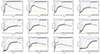 |
Fig. A.1. Same as the bottom-left panel of Fig. 2, but for the entire model set computed with the radiation hydrodynamics code HERACLES. The model parameters are discussed in Sect. 2.1 and given in Table 1. |
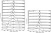 |
Fig. A.2. Evolution of the spectral region centered on the rest wavelength of Hβ (left) and He II 5411.52 Å (right) for model mdot0p01/rcsm8e14 (see Fig. 3 for the results obtained for Hα and Fig. 5 for He II 4685.70 Å). |
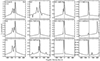 |
Fig. A.3. Mosaic showing various lines of H I, He I, He II, C III, C IV, and N IV for the reference model mdot0p01/rcsm8e14 at 1 d. In all cases, the x-axis covers from ± 500 km s−1 but the y-axis covers a wide range of normalized fluxes, with very strong narrow emission lines like Hα and much weaker ones like N IV 7122.98 Å. |
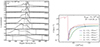 |
Fig. A.4. Left: Same as Fig. 10, but for the model counterpart with a greater RCSM value of 4 × 1014 cm. Right: Illustration of the velocity profile versus radius for the models discussed in Sect. 4.3 and whose density profiles are shown in the bottom panel of Fig. 1. |
All Tables
All Figures
|
Fig. 1. Radial profiles of the mass density used as initial conditions for our radiation-hydrodynamics calculations. From top to bottom, we show groups of models varying in RCSM, Ṁ, and wind velocity profile (i.e., βw and V∞). Radial profiles of the velocity are shown for the last model group in the right panel of Fig. A.4. See Sect. 2.1 and Table 1 for additional information. |
| In the text | |
|
Fig. 2. Illustration of radiation and hydrodynamical properties computed by HERACLES for model mdot0p01/rcsm8e14. Top row: Variation in the velocity at multiple epochs versus radius (top left) and versus the distance above the shock (top right). Bottom left: Evolution of the velocity of “mass parcels” initially at radii 0.1, 0.2, 0.35, 0.5, 0.7, 1.0, 1.5, and 3.95 × 1015 cm (the last radius is near the outer grid boundary) and over the full duration of 15 d of the HERACLES simulation. The solid line shows the value of this velocity as read in directly from the simulation. The dashed line shows the same quantity but estimated through a time integral of the radiative acceleration (see the discussion in Sect. 3.1). In all cases, the two curves agree closely until the mass parcel is shocked, which corresponds to the near-vertical jump of the solid lines. The black circles and the stars indicate the velocity at the location where the electron-scattering optical depth is 2/3 (i.e., the photosphere) and at 0.01. Bottom right: Counterpart of the top-left panel but for the luminosity (i.e., quantity Lr = 4πr2Fr). Only the inner half of the grid is shown. |
| In the text | |
|
Fig. 3. Evolution of the spectral region centered on the rest wavelength of Hα for model mdot0p01/rcsm8e14. The symmetric solid vertical lines on each side of the origin correspond to the velocity at the location in the unshocked CSM where the electron-scattering optical depth is 0.01, thus exterior to the location of the photosphere. The dashed vertical lines correspond to ± V∞ of the original, unadulterated CSM. The spectral evolution in other H I Balmer lines is analogous to that shown here for Hα (see the case of Hβ shown in the left panel of Fig. A.2). Note that He II 6560.09 Å contributes some flux on the blue edge of Hα, well separated from it initially but overlapping with the Hα emission at 2–5 d. The ordinate range changes in each panel for better visibility. |
| In the text | |
|
Fig. 4. Same as Fig. 3, but for He I 5875.66 Å. This line is present at early times until about 1 d and then again after ∼3 d, but absent between, when the ionization of the unshocked CSM is too high. |
| In the text | |
|
Fig. 5. Same as Fig. 3, but for He II 4685.70 Å. This line is essentially unblended and present until ∼5 d, after which the He ionization is too low. The symmetric solid vertical lines on each side of the origin correspond here to the velocity at the location in the unshocked CSM where the electron-scattering optical depth is 0.1. |
| In the text | |
|
Fig. 6. Same as Fig. 3, but for C IV 5801.31 Å. Here, the solid vertical bars on each side of the origin correspond to the velocity at the location in the unshocked CSM where the electron-scattering optical depth is 0.1. |
| In the text | |
|
Fig. 7. Same as Fig. 3, but for N IV 7122.98 Å. This line is absent prior to ∼1 d and after ∼5 d, because of the unsuitable ionization state of the unshocked CSM at those epochs. This spectral region contains other N IV lines at 7109.35, 7111.28, and 7127.25 Å. Here, the solid vertical bars on each side of the origin correspond to the velocity at the location in the unshocked CSM where the electron-scattering optical depth is 0.1. |
| In the text | |
|
Fig. 8. Same as Fig. 3, but for C III 5695.92 Å. Besides the evolution of that line in width caused by the radiative acceleration of the unshocked CSM, its strength also varies in time with a minimum around 1.5 d caused by the high ionization of the unshocked CSM (at those epochs, C IV is the dominant ion). |
| In the text | |
|
Fig. 9. Results from the radiation-hydrodynamics calculations for models differing in RCSM. Top: Bolometric luminosity recorded at the outer boundary and starting when the power exceeds 1041 erg s−1. Middle: Same as top for the cumulative bolometric luminosity. Here, we use the HERACLES time modified for the light-travel time to the outer boundary. Bottom: Evolution of the velocity at the location in the unshocked CSM where the electron-scattering optical depth is 0.01. When that location is shocked, we report the velocity at the radius immediately exterior to the shock. |
| In the text | |
|
Fig. 10. Evolution of the spectral region centered on the rest wavelength of Hα for model mdot0p01/rcsm2e14. The symmetric solid vertical lines on each side of the origin correspond to the velocity at the location in the unshocked CSM where the electron-scattering optical depth is 0.01. The dashed vertical lines correspond to ±V∞, where V∞ is the terminal wind velocity of the original, unadulterated CSM. |
| In the text | |
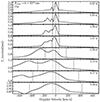 |
Fig. 11. Same as Fig. 10, but for the model counterpart with a greater RCSM value of 6 × 1014 cm. |
| In the text | |
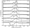 |
Fig. 12. Same as Fig. 10, but for the model counterpart with the largest RCSM value of 1015 cm. |
| In the text | |
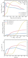 |
Fig. 13. Same as Fig. 9, but for the model set differing in CSM density (i.e., Ṁ). |
| In the text | |
|
Fig. 14. Same as Fig. 10, but for models differing in Ṁ, covering from low (top panel) to high mass loss rates (bottom panel). |
| In the text | |
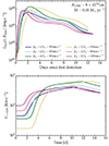 |
Fig. 15. Close counterpart to Fig. 9, but for models differing in βw and V∞. |
| In the text | |
|
Fig. 16. Same as Fig. 10, but for two models differing in the original CSM velocity V∞ with a value of 20 km s−1 (top panel) and 120 km s−1 (bottom panel). |
| In the text | |
|
Fig. 17. Evolution of the broad and narrow emission components in the Hα spectral region from ∼0.5 d until ∼15 d after shock breakout for model rcsm2e14 (left) and rcsm8e14 (right). The symmetric solid vertical lines on each side of the origin correspond to the velocity at the location in the unshocked CSM where the electron-scattering optical depth is 0.01. For the CDS velocity of ∼6000 km s−1 in the rcsm8e14 model, the He I 6678 Å trough extends out to the Hα rest wavelength and thus may overlap with a narrow Hα component. |
| In the text | |
|
Fig. A.1. Same as the bottom-left panel of Fig. 2, but for the entire model set computed with the radiation hydrodynamics code HERACLES. The model parameters are discussed in Sect. 2.1 and given in Table 1. |
| In the text | |
|
Fig. A.2. Evolution of the spectral region centered on the rest wavelength of Hβ (left) and He II 5411.52 Å (right) for model mdot0p01/rcsm8e14 (see Fig. 3 for the results obtained for Hα and Fig. 5 for He II 4685.70 Å). |
| In the text | |
|
Fig. A.3. Mosaic showing various lines of H I, He I, He II, C III, C IV, and N IV for the reference model mdot0p01/rcsm8e14 at 1 d. In all cases, the x-axis covers from ± 500 km s−1 but the y-axis covers a wide range of normalized fluxes, with very strong narrow emission lines like Hα and much weaker ones like N IV 7122.98 Å. |
| In the text | |
|
Fig. A.4. Left: Same as Fig. 10, but for the model counterpart with a greater RCSM value of 4 × 1014 cm. Right: Illustration of the velocity profile versus radius for the models discussed in Sect. 4.3 and whose density profiles are shown in the bottom panel of Fig. 1. |
| In the text | |
Current usage metrics show cumulative count of Article Views (full-text article views including HTML views, PDF and ePub downloads, according to the available data) and Abstracts Views on Vision4Press platform.
Data correspond to usage on the plateform after 2015. The current usage metrics is available 48-96 hours after online publication and is updated daily on week days.
Initial download of the metrics may take a while.