| Issue |
A&A
Volume 694, February 2025
|
|
|---|---|---|
| Article Number | A137 | |
| Number of page(s) | 15 | |
| Section | Planets, planetary systems, and small bodies | |
| DOI | https://doi.org/10.1051/0004-6361/202452699 | |
| Published online | 10 February 2025 | |
Transit-timing variations in the AU Mic system observed with CHEOPS★
1
Konkoly Observatory, HUN-REN Research Centre for Astronomy and Earth Sciences,
Konkoly Thege út 15–17,
1121
Budapest,
Hungary
2
CSFK, MTA Centre of Excellence, Budapest,
Konkoly Thege út 15–17,
1121
Budapest,
Hungary
3
HUN-REN-ELTE Exoplanet Research Group,
Szent Imre h. u. 112,
Szombathely
9700,
Hungary
4
ELTE Gothard Astrophysical Observatory,
9700
Szombathely,
Szent Imre h. u. 112,
Hungary
5
INAF, Osservatorio Astronomico di Padova,
Vicolo dell’Osservatorio 5,
35122
Padova,
Italy
6
Dipartimento di Fisica, Università degli Studi di Torino,
via Pietro Giuria 1,
10125
Torino,
Italy
7
Observatoire astronomique de l’Université de Genève,
Chemin Pegasi 51,
1290
Versoix,
Switzerland
8
European Space Agency (ESA), European Space Research and Technology Centre (ESTEC),
Keplerlaan 1,
2201 AZ
Noordwijk,
The Netherlands
9
Department of Physics, University of Warwick,
Gibbet Hill Road,
Coventry
CV4 7AL,
UK
10
Department of Astronomy, Stockholm University, AlbaNova University Center,
10691
Stockholm,
Sweden
11
Astronomical Institute, Slovak Academy of Sciences,
05960
Tatranská Lomnica,
Slovakia
12
Center for Space and Habitability, University of Bern,
Gesellschaftsstrasse 6,
3012
Bern,
Switzerland
13
Space Research and Planetary Sciences, Physics Institute, University of Bern,
Gesellschaftsstrasse 6,
3012
Bern,
Switzerland
14
Instituto de Astrofísica de Canarias,
Vía Láctea s/n,
38200
La Laguna,
Tenerife,
Spain
15
Departamento de Astrofísica, Universidad de La Laguna,
Astrofísico Francisco Sanchez s/n,
38206
La Laguna,
Tenerife,
Spain
16
Admatis,
5. Kandó Kálmán Street,
3534
Miskolc,
Hungary
17
Depto. de Astrofísica, Centro de Astrobiología (CSIC-INTA), ESAC campus,
28692
Villanueva de la Cañada (Madrid),
Spain
18
Instituto de Astrofisica e Ciencias do Espaco, Universidade do Porto, CAUP, Rua das Estrelas,
4150-762
Porto,
Portugal
19
Departamento de Fisica e Astronomia, Faculdade de Ciencias, Universidade do Porto, Rua do Campo Alegre,
4169-007
Porto,
Portugal
20
Space Research Institute, Austrian Academy of Sciences,
Schmiedlstrasse 6,
8042
Graz,
Austria
21
Centre for Exoplanet Science, SUPA School of Physics and Astronomy, University of St Andrews,
North Haugh,
St Andrews
KY16 9SS,
UK
22
CFisUC, Departamento de Física, Universidade de Coimbra,
3004516
Coimbra,
Portugal
23
Institute of Planetary Research, German Aerospace Center (DLR),
Rutherfordstrasse 2,
12489
Berlin,
Germany
24
INAF, Osservatorio Astrofisico di Torino,
Via Osservatorio, 20,
10025
Pino Torinese,
To,
Italy
25
Centre for Mathematical Sciences, Lund University,
Box 118,
221 00
Lund,
Sweden
26
Aix Marseille Univ, CNRS, CNES, LAM,
38 rue Frédéric Joliot-Curie,
13388
Marseille,
France
27
SRON Netherlands Institute for Space Research,
Niels Bohrweg 4,
2333 CA
Leiden,
The Netherlands
28
Centre Vie dans l’Univers, Faculté des sciences, Université de Genève,
Quai Ernest-Ansermet 30,
1211
Genève 4,
Switzerland
29
Leiden Observatory, University of Leiden,
PO Box 9513,
2300 RA
Leiden,
The Netherlands
30
Department of Space, Earth and Environment, Chalmers University of Technology, Onsala Space Observatory,
439 92
Onsala,
Sweden
31
National and Kapodistrian University of Athens, Department of Physics, University Campus,
Zografos
157 84,
Athens,
Greece
32
Astrobiology Research Unit, Université de Liège,
Allée du 6 Août 19C,
4000
Liège,
Belgium
33
Department of Astrophysics, University of Vienna,
Türkenschanzstrasse 17,
1180
Vienna,
Austria
34
Division Technique INSU,
CS20330,
83507
La Seyne sur Mer cedex,
France
35
Institute for Theoretical Physics and Computational Physics, Graz University of Technology,
Petersgasse 16,
8010
Graz,
Austria
36
Konkoly Observatory, Research Centre for Astronomy and Earth Sciences,
1121
Budapest,
Konkoly Thege Miklós út 15–17,
Hungary
37
ELTE Eötvös Loránd University, Institute of Physics,
Pázmány Péter sétány 1/A,
1117
Budapest,
Hungary
38
Lund Observatory, Division of Astrophysics, Department of Physics, Lund University,
Box 118,
22100
Lund,
Sweden
39
IMCCE, UMR8028 CNRS, Observatoire de Paris, PSL Univ., Sorbonne Univ.,
77 av. Denfert-Rochereau,
75014
Paris,
France
40
Institut d’astrophysique de Paris, UMR7095 CNRS, Université Pierre & Marie Curie,
98bis blvd. Arago,
75014
Paris,
France
41
Astrophysics Group, Lennard Jones Building, Keele University,
Staffordshire
ST5 5BG,
UK
42
European Space Agency, ESA – European Space Astronomy Centre,
Camino Bajo del Castillo s/n,
28692
Villanueva de la Cañada, Madrid,
Spain
43
INAF, Osservatorio Astrofisico di Catania,
Via S. Sofia 78,
95123
Catania,
Italy
44
Institute of Optical Sensor Systems, German Aerospace Center (DLR),
Rutherfordstrasse 2,
12489
Berlin,
Germany
45
Weltraumforschung und Planetologie, Physikalisches Institut, University of Bern,
Gesellschaftsstrasse 6,
3012
Bern,
Switzerland
46
Dipartimento di Fisica e Astronomia “Galileo Galilei”, Università degli Studi di Padova,
Vicolo dell’Osservatorio 3,
35122
Padova,
Italy
47
ETH Zurich, Department of Physics,
Wolfgang-Pauli-Strasse 2,
8093
Zurich,
Switzerland
48
Cavendish Laboratory,
JJ Thomson Avenue,
Cambridge
CB3 0HE,
UK
49
Institut fuer Geologische Wissenschaften, Freie Universitaet Berlin,
Maltheserstrasse 74-100,
12249
Berlin,
Germany
50
Institut de Ciencies de l’Espai (ICE, CSIC),
Campus UAB, Can Magrans s/n,
08193
Bellaterra,
Spain
51
Institut d’Estudis Espacials de Catalunya (IEEC),
08860
Castelldefels (Barcelona),
Spain
52
Weltraumforschung und Planetologie, Physikalisches Institut, University of Bern,
Sidlerstrasse 5,
3012
Bern,
Switzerland
53
ESOC, European Space Agency,
Robert Bosch Str. 5,
64293
Darmstadt,
Germany
54
Space sciences, Technologies and Astrophysics Research (STAR) Institute, Université de Liège,
Allée du 6 Août 19C,
4000
Liège,
Belgium
55
Institute of Astronomy, University of Cambridge,
Madingley Road,
Cambridge
CB3 0HA,
UK
56
Leibniz Institute for Astrophysics,
An der Sternwarte 16,
14482
Potsdam,
Germany
★★ Corresponding author; This email address is being protected from spambots. You need JavaScript enabled to view it.
Received:
22
October
2024
Accepted:
8
January
2025
Abstract
Context. AU Mic is a very active M dwarf star with an edge-on debris disk and two known transiting sub-Neptunes with a possible third planetary companion. The two transiting planets exhibit significant transit-timing variations (TTVs) that are caused by the gravi tational interaction between the bodies in the system.
Aims. Using photometrical observations taken with the CHaracterizing ExOPlanet Satellite (CHEOPS), we aim to constrain the plan etary radii, the orbital distances, and the periods of AU Mic b and c. Furthermore, our goal is to determine the superperiod of the TTVs for AU Mic b and to update the transit ephemeris for both planets. Additionally, based on the perceived TTVs, we study the possible presence of a third planet in the system.
Methods. We conducted ultra-high precision photometric observations with CHEOPS in 2022 and 2023. We used Allesfitter to fit the planetary transits and to constrain the planetary and orbital parameters. We combined our new measurements with results from previous years to determine the periods and amplitudes of the TTVs. We applied dynamical modelling based on TTV measurements from the 2018–2023 period to reconstruct the perceived variations.
Results. We found that the orbital distances and periods for AU Mic b and c agree with the results from previous works. However, the values for the planetary radii deviate slightly from previous values, which we attribute to the effect of spots on the stellar surface. AU Mic c showed very strong TTVs, with transits that occurred ∼80 minutes later in 2023 than in 2021. Through a dynamical analysis of the system, we found that the observed TTVs can be explained by a third planet with an orbital period of ∼12.6 days and a mass of 0.203−0.024+0.022 M⊕. We explored the orbital geometry of the system and found that AU Mic c has a misaligned retrograde orbit. The limited number of AU Mic observations prevented us from determining the exact dynamical configuration and planetary parameters. Further monitoring of the system with CHEOPS might help to improve these results.
Key words: planets and satellites: fundamental parameters
This article uses data from the CHEOPS programme CH_PR100010.
© The Authors 2025
 Open Access article, published by EDP Sciences, under the terms of the Creative Commons Attribution License (https://creativecommons.org/licenses/by/4.0), which permits unrestricted use, distribution, and reproduction in any medium, provided the original work is properly cited.
This article is published in open access under the Subscribe to Open model. This email address is being protected from spambots. You need JavaScript enabled to view it. to support open access publication.
1 Introduction
AU Mic is a young M1-type dwarf star with an age of 22±3 Myr (Mamajek & Bell 2014) that hosts two sub-Neptune-type planets (Plavchan et al. 2020; Martioli et al. 2021) and a complex debris disk that is viewed edge-on (Mathioudakis & Doyle 1991; Kalas et al. 2004). It is a fairly close system with a distance of 9.71 pc (Gaia Collaboration 2023), which makes it an excellent target for investigating a planetary system in the early stages of evolution.
AU Mic is a very active M dwarf star (Butler et al. 1981; Tsikoudi & Kellett 2000; Gilbert et al. 2022) with a strong magnetic field (Kochukhov & Reiners 2020). It produces frequent flare events (Ilin & Poppenhaeger 2022) and has large stellar spots (Hebb et al. 2007; Plavchan et al. 2020). Given the relative proximity of the planets to the host star, signs of star-planet interactions are expected (Kavanagh et al. 2021) and may be reflected in the distribution of stellar flares (Ilin & Poppenhaeger 2022). On the other hand, the spots on the stellar surface may influence the planetary parameters derived from transit modelling for AU Mic b and c (Oshagh et al. 2013). A better understanding of the activity of the host may therefore be beneficial for refined radii of the planets. We study the activity of AU Mic in an accompanying publication (Kriskovics et al., in prep.).
AU Mic hosts an extended debris disk that is viewed edge-on (Kalas et al. 2004). Infrared observations confirmed the size of the disk, which has an inner radius of about 9 AU (MacGregor et al. 2013; Matthews et al. 2015) and a peak brightness of about 40 AU (MacGregor et al. 2013). Its outer halo extends to 210 AU (Kalas et al. 2004). The disk exhibits complex structures from large radial cavities to clumps and warps. It also shows asymmetries in the vertical distribution of the dust (Schneider et al. 2014; Wisniewski et al. 2019).
The two known transiting planets in the system, AU Mic b and c, are both Neptune-sized bodies, with masses of 11.7±5.0 M⊕ and 22.2±6.7 M⊕, respectively (Zicher et al. 2022). The radii of planets b and c were determined to be 3.55±0.13 R⊕ and 2.56±0.12 R⊕ (Szabó et al. 2022), respectively. However, because of the strong activity and the spot-covered surface of the host star AU Mic, the precision of the estimates on the planetary radii may be lower. The inner planet, AU Mic b, has a mean orbital period of about 8.463 days (Gilbert et al. 2022) and is in a 7:4 spin-orbit resonance with the star (Szabó et al. 2021). The outer planet, AU Mic c, has a mean orbital period of 18.859 days (Gilbert et al. 2022). Both planets exhibit significant transittiming variations (TTVs) of the order of tens of minutes (Szabó et al. 2022). These large variations are likely due to the gravitational effects of additional planets in the system. Wittrock et al. (2023) found that the observed TTVs could be explained with an Earth-sized planet that orbits between AU Mic b and c. A more precise determination of the superperiod of the TTVs may help us to confirm the presence of AU Mic d.
The CHaracterizing ExOPlanet Satellite (CHEOPS) is a small-class ESA mission with the primary objective of conducting follow-up studies of known exoplanetary systems using ultra-high precision photometry (Benz et al. 2021). With its observational strategy, stability, the effective aperture of 30 cm, and the broad bandpass of 330–1100 nm (Deline et al. 2020), CHEOPS is suitable for detecting planetary transits over an extended portion of the sky around a large variety of host stars (Fortier et al. 2024). In recent years, CHEOPS has proven to be a valuable tool for constraining planetary radii (Lendl et al. 2020; Delrez et al. 2021; Bonfanti et al. 2021) and determining TTV in multiplanet systems (Szabó et al. 2022; Delrez et al. 2023).
We present high-precision photometric observations of the transits of AU Mic b and c that were carried out by CHEOPS. In Sect. 2, we describe our observations and data reduction methods. In Sect. 3, we analyse the transit light curves and describe the dynamical analysis of the system based on the TTV measurements. We present and discuss our results in Sect. 4.
2 Observations and data reduction
2.1 CHEOPS photometry
We observed six and three transits of AU Mic b and c during the observation period 2022, respectively. In 2023, seven additional transits were observed by CHEOPS for AU Mic b, and four more transit for AU Mic c. On two occasions, a double transit of both planets b and c was observed, once in each year. Since AU Mic is a relatively bright star with a brightness of G=7m. 843 in the Gaia G band (Gaia Collaboration 2023), it was possible to perform short-cadence photometry (with exposures of 3 seconds). However, due to the strong flaring activity of the star, only eight transits of planet b and six for planet c were appropriate for further analysis following visual inspection. The efficiency of the observations varied between 50.2–79.1% in 2022 and 50.0– 79.3% in 2023. The observation log for the entire campaign of 2022–2023 is available here.
In this analysis, photometry was extracted using the CHEOPS imagettes alone. The imagettes are small images centred around the target star, with a radius of 30 pixels, and unlike sub-array images, they do not have to be co-added on board of the telescope. They can instead be downloaded individually. Photometric extraction of imagettes was carried out using PSF imagette photometric extraction (PIPE), a tool that was specifically developed for this purpose using point-spread function (PSF) photometry (Brandeker et al. 2024). In this case, the PIPE photometry has a shorter cadence than the CHEOPS data reduction pipeline (DRP) on the aperture photometry of the subarrays, but the signal-to-noise ratio (S/N) is similar. The shorter cadence of the imagettes can be of crucial importance in the case of active stars, such as AU Mic, to better identify and adequately analyse flares. We provide a detailed analysis of the flares of AU Mic in an accompanying publication (Kriskovics et al., in prep.).
Since CHEOPS continuously rolls during its 98.77-minute orbit in order to keep the radiators from facing towards Earth, the field of view of the telescope also rotates around the target. This effect, combined with the irregularly shaped CHEOPS PSF, causes systematic variations in the background flux in phase with the roll angle, which has to be appropriately handled before the data are analysed.
AU Mic belongs to the most active stars, which are characterised by very frequent energetic flares and usually complex flares. All transit light curves were contaminated by more or less separated short flares, which could have been successfully removed before the fitting process with Allesfitter, described in Sect. 3.1. However, several transit light curves of both AU Mic b and AU Mic c were compromised by long- lasting flare complexes that occurred very close to the transit or appeared during the transit. Their contamination deteriorated the transit shape so much they could not be reliably separated if the precision of the parameters from clearer transits was to be achieved. Therefore, we decided to remove these severely contaminated transits from the transit analysis. The CHEOPS light curves of the transits we selected for parameter fitting are shown in Fig. 1, and the transit light curves that we omitted because of severe flare contamination are plotted in Fig. A.1.
2.2 Pre-processing of the light curves
The CHEOPS light curves of AU Mic were corrected for rollangle systematics using a parametric estimation derived from the data, with the photometric points phased by the roll angle. After we mased out the transits and the evident flares, the data were phased in the roll-angle domain. A further 2.5σ clipping was applied to exclude outliers such as potential flares and lightcurve transients. The roll systematics model was a sixth-order Fourier polynomial, whose coefficients were determined by a least-squares fit to the phased out-of-transit points, and we then subtracted the derived parametric model from the entire dataset. The corrected data set was then used as input for the light-curve modeller.
This correction method was simpler than the non-parametric models we applied in our earlier work (e.g. Szabó et al. 2021) because the new-generation fitting algorithms can properly handle the flares and the high-order residuals of the rolling systematics that survived the subtraction of the Fourier polynomial. We achieved a more reliable estimate of the planet parameter uncertainties and a more robust handling of the data in general by letting the fitting procedure separate the various systematics in the light curve.
The flares of AU Mic are known to appear frequently, and their amplitude can well exceed the transit depth of the planets. Quite often, several flares merge into a flare complex with a timescale commensurable to the duration of the transits (Szabó et al. 2021, 2022). The flares can therefore introduce biases in the estimation of the baseline flux (which propagates to the transit parameters, most importantly, the transit depth), and if they appear during the transit, they can compress the transit depth and distort the shape of the light curve.
To filter out flares, manual removal was followed in our earlier publications (Szabó et al. 2021, 2022). In this current work, we changed this to a semi-automated process. First, light-curve segments that certainly had significant flares were marked by an artificial-intelligence application, which is the same process as for collecting the database of AU Mic flares for a dedicated analysis (see Kriskovics et al., in prep. for more details). The marked segments of the light curve were then removed. In the next step, we repeated the manual flare-removal process that we followed in our earlier publications, and we removed the low-amplitude flares that were not identified by the AI algorithms, with the aim of filtering out all suspicious light curve parts and possible biases due to flares from the analysis. Figure 1 shows the phased transit light curves after the complete flare-filtering process, and this data set was the input for the light-curve analysis.
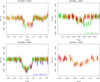 |
Fig. 1 Phased transit light curves of the 2022 and 2023 measurements of the AU Mic b (left panels) and c transits (right panels) after flare removal. The ephemeris and period used here are T0,b = 2458 330.38416d and Pb = 8.4631427d, and T0,c = 2459454.8973 BJD, Pc = 18.85882 d. The TTV is very prominent for both planets compared to the earlier ephemeris. AU Mic b transited after the AU Mic c transit on 22 August 2022 (top right panel), and similarly, planet c transited after planet b on 21 September 2023 (bottom left panel). |
3 Data analysis
3.1 Refining the transit parameters
In order to derive orbital and planetary parameters of AU Mic b and c based on the CHEOPS photometry, we employed the Allesfitter1 software package (Günther & Daylan 2019, 2021). This is a public software for modelling photometric and radial-velocity (RV) data. It can accommodate multiple exoplanets, multi-star systems, star spots, stellar flares, transit-time variations, and various noise models. It automatically runs a nested- sampling or Markov chain Monte Carlo fit. We opted for the nested-sampling fit with default settings. Several fundamental parameters were optimised during the fitting procedure, including the reference mid-transit time Tc , the orbital period Porb, the planet-to-star radius ratio Rp /Rs , the scaled sum of the fractional radii (Rp + Rs)/a, and the cosine of the orbit inclination angle (cos i). The quadratic limb-darkening (LD) law was applied during the fitting procedure. The u1 and u2 LD coefficients were first linearly interpolated based on the stellar parameters of Teff = 3665 ± 31 K and log g = 4.52 ± 0.05 [cgs] found by Donati et al. (2023). We used the tables of coefficients calculated for the CHEOPS passband using the PHOENIX-COND models by Claret (2021). We then converted these LD coefficients into q1 and q2 (Kipping 2013). The q1 and q2 parameters were fitted during the procedure. In order to model the flux baseline, we applied a Gaussian process (GP) regression method using the SHOTerm (simple harmonic oscillator – SHO) plus JitterTerm kernel, implemented in the Celerite2 (Kallinger et al. 2014; Foreman- Mackey et al. 2017; Barros et al. 2020) package, with a fixed quality factor of  , as is common for quasi-periodic stellar variability. The regression was made by using log ω0 and log S0 with bounds on the values of these parameters to be input by the user. The parameter log ω0 reflects the frequency (period), and log S0 reflects the scaled power (amplitude) of the signal. The instrumental noise in the CHEOPS data was sampled using the log σ parameter. We assumed a circular orbit of AU Mic b and c.
During the analysis with Allesfitter, we followed the strategy described below. We simultaneously fitted all AU Mic b and c transits per observing year, that is, the transits from 2022 and 2023 were fitted separately. The main reason for splitting the data into two groups was the possibility of comparing the evolution of the transit parameters of the planets. In most cases, we applied broad uniform priors on the parameters. The applied priors and the fitted parameters are listed in Table 1 and the derived parameters are listed in Table 2. The corresponding transit light curves, overplotted with the best-fitting Allesfitter models, are shown in Fig. 2.
Overview of the Allesfitter priors and best-fitting parameters of AU Mic b and c obtained based on the data from 2022 and 2023.
3.2 TTV analysis
The O – C diagrams of the transit mid-time for AU Mic b and c are shown in Fig. 3. Observations from previous years are complemented with CHEOPS data from the 2022 and 2023 observation periods. Both planets showed large-amplitude TTVs, and planet c deviated significantly from those of previous years. The difference between the mid-transit times reached ~90 minutes. Tables 3 and 4 show the exact mid-transit times and O – C values for planets b and c, respectively. Based on Tc = 2458 330.38416 d and Pmean = 8.4631427 d for planet b and Tc = 2459454.8973 and Pmean = 18.85882 d for planet c. The superperiod of the TTVs exhibited by planet b (according to the fit in Fig. 3) is 1150 days, which is slightly shorter than reported in Szabó et al. (2022). The reason is the longer dataset that is now available (almost 1.5 superperiods) than was the case of the analysis in Szabó et al. (2022) (less than one superperiod), and the pattern is better defined. The peak-to-peak TTV amplitude of the best-fit periodic TTV model to AU Mic b is 24.5 minutes, which agrees well with the predictions in Szabó et al. (2022). The presence of a third planet, AU Mic d, has been suggested by Wittrock et al. (2023) based on TTV signals. In order to test this possibility, we conducted dynamical simulations assuming a third planet in the system.
We used TRADES3 (Borsato et al. 2014, 2019, 2021), a Fortran90-Python software, to model four configurations of the AU Mic system. In the initial configuration (1), we focused exclusively on the system comprising the two transiting planets, b and c, and only modelled the transit times during the orbital integration. In the subsequent two configurations (2) and (3), we additionally incorporated planet d (Wittrock et al. 2023), and as for (1), we only modelled the transit times of b and c. Only in the fourth configuration (4) did we also include the SERVAL RVs from Zicher et al. (2022). Another difference between the four configurations is the parameters that were fitted in the analysis. Generally, we set the stellar mass from Plavchan et al. (2020), and fitted (as in Nascimbeni et al. 2023) for the planet-to-star mass ratios (Mp /M⋆), the periods (P), the eccentricities (e) and argument of pericenters (ω) in the form  , and the mean longitude (λ4) for all the planets. We fitted the longitude of the ascending node (Ω) of planet c in all four configurations, and of d in configurations (2), (3), and (4). The inclination (i) of planet c in configurations (3), (4) and of d in (2), (3), and (4) was fitted as well. In configuration (4) we also fitted for an RV offset (γ) and a jitter term (in log2). The RV data are characterised by strong activity; but by default, TRADES does not implement an activity model. Because the problem is so complex, we decided not to test it. The total numbers of fitted parameters were 11, 18, 19, and 21 for configurations (1), (2), (3), and (4), respectively. All parameters were defined at the reference time BJDTDB – 2450000 = 8329. All priors on the parameters are listed in Table B.1 The parameters of b and c were set to the values in Table 2, and Ωb was set to 180° (assuming the same reference system as in Winn 2010 and adopted in Borsato et al. 2014).
For each configuration, we first performed a run of TRADES with PYDE (Parviainen et al. 2016) allowing for 200 000 steps and used the best-fit configuration set as a starting point for EMCEE (Foreman-Mackey et al. 2013). Then we ran EMCEE for 1 000 000 steps (with a conservative thinning factor of 100). For each configuration, we used as walkers for EMCEE the same number of parameter sets as used in PYDE, 100 for configurations (1), (2), and (3), and 2005 for (4). Within EMCEE we used a 80% ÷ 20% combination of the differential evolution (Nelson et al. 2014) and snooker (ter Braak & Vrugt 2008) proposal samplers. After we confirmed that the chains converged through visual inspection, auto-correlation function (ACF), Gelman-Rubin statistics (Gelman & Rubin 1992), and the Geweke criterion (Geweke 1991), we discarded the first 350 000, 500 000, 600 000, and 800 000 steps as burn-in for configurations (1), (2), (3), and (4), respectively.
We computed the high-density interval (HDI) at 68.27% as the 1σ equivalent for each fitted and physical parameter of the posterior distribution. We defined the maximum-a-posteriori (MAP) configuration set as the best-fit parameter, that is, the set of parameters that maximised the log-probability6 ln P, whose parameters were completely within all fitted 1σ HDI. The best-fit solution with 100 random samples drawn from the 1σ posterior distribution is shown in Figs. B.1, B.2, B.3, and B.4 with the O – C plots for planets b and c for all four configurations, and the RV model in Fig. B.5 for configuration (4).
Overview of the Allesfitter-derived parameters of AU Mic b and c obtained based on the data from 2022 and 2023.
4 Results and discussion
4.1 Fundamental planetary parameters
In Tables 5 and 6, we compare the fundamental transit parameters observed between 2018 and 2023, taken from this paper and from five earlier analyses in the literature. Here, Plavchan et al. (2020) contains the analysis of 2018 TESS data, Gilbert et al. (2022) and Martioli et al. (2021) are based on the combined TESS 2018–2020 data, and Szabó et al. (2021) and Szabó et al. (2022) are based on the CHEOPS observations from 2020 and 2021, respectively. We sorted the table columns according to the time of observation; and therefore, moving from left to right, the columns show the measurements in a decreasing order of the time of the observations.
Most parameters are consistent within the uncertainties, with the important exceptions of Rp /Rs and b for planet b. In the case of AU Mic b, the Rp/Rs parameter was found to be smaller in 2022 than in 2023 (0.0470 versus 0.0517). The transit depth in 2022 was slightly larger than what we observed in 2021 (0.0433±0.001, Szabó et al. 2022), while it was determined to be in the interval of 0.0512–0.0531 in 2018 and 2020 (Szabó et al. 2022), which is compatible to the transit depth parameter that we observed in 2023. The transit depth parameters of AU Mic c are comparable to each other, with a slight decrease in the 2023 value.
The impact parameter b has an average value of 0.22 in the case of AU Mic b, but since the 2023 CHEOPS data and 2020 CHEOPS data are two outliers (with values of 0.386 and 0.09, respectively), the dataset is barely consistent. The values for the impact parameter of AU Mic c are consistent within the uncertainties, but appear to be slightly higher in the case of the more recent CHEOPS data.
We followed the working hypothesis that the main reason for the varying transit parameters of the two planets can be the actual realisation of the spot distribution on the surface and their biases on the transit shape (Szabó et al. 2021). This is also corroborated by the observation that CHEOPS measurements seem to be more strongly biased (more year-to-year variations) than the TESS measurements, and CHEOPS is bluer and more sensitive to inhomogeneities in the surface temperature. Therefore, assuming a common reason behind the biases and expecting similarities (correlation, anti-correlation, at least in part) in the actual values of the parameters, we tested a possible correlation between the transit depth and the impact parameters of AU Mic b and c, and also possible correlations between the same parameter (Rp/Rs and impact parameter of the two planets in comparison). We calculated Pearson’s correlation coefficient (testing linear dependence) and Spearman’s rank correlation coefficient (testing any monotonic dependence). We found no significant correlation (a coefficient value of zero was always within the error interval, and we also observed p > 0.1 in all cases). However, the lack of a significant correlations does not rule out activity as a reason for the observed biases of the parameters, but is instead a result of the low number statistics, which is still not enough for a conclusive result. This will be better determined in the future when AU Mic has been observed for more years.
The observed instability of the transit parameters on a timescale of years confirms our observation that the transit parameter depends significantly on the actual spot pattern on the stellar disk, which is reproducible (we see similar biases for transits that repeat at similar stellar rotational longitudes; Szabó et al. 2021). This proves that in case of AU Mic, the transit depth parameter is not exclusively characteristic of the planet itself, but the actual spot distribution causes bias the observed value. (Hence, calling it the “transit depth parameter” is more accurate because it is an Rp /Rs value, but biased by the actual spot distribution).
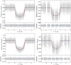 |
Fig. 2 Stacked and binned CHEOPS transit light curves of AU Mic b (left panels) and AU Mic c (right panels) from 2022 (top panels) and from 2023 (bottom panels), overplotted with the best-fitting Allesfitter models (20 curves from random posterior samples). The residuals are also shown. |
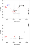 |
Fig. 3 TTV diagrams of AU Mic b (upper panel) calculated with Tc = 2458 330.38416 and Pmean = 8.4631427 d, and AUMic c (lower panel) calculated with Tc = 2 459 454.8973 and Pmean = 18.85882 d. We included Transiting Exoplanet Survey Satellite (TESS, red symbols), Spitzer (blue symbols), Earth-based Pan-STARRS (light grey symbols) and CHEOPS (black symbols) measurements. The harmonic fit to AU Mic b data (dotted red line) illustrates the most probable shape of a periodic TTV fitted to the data. This is shown to illustrate the trend of the distribution without any dynamical interpretation. |
4.2 Possible solutions for AU Mic d and concluding remarks
The parameters of the planets in the AU Mic system based on the dynamical analysis are shown in Table B.1. Configuration (1), in which only two planets, b and c, were assumed, is unable to explain the observed TTVs, as shown in Fig. B.1 and in the first column of Table B.1. We found that in accordance with Wittrock et al. (2023), the TTVs exhibited by planets b and c can be explained by the presence of an additional third planetary body in the system on an orbit that falls between the orbits of the two transiting planets. It is worth noting, however, that the shapes and amplitudes of the fitted TTV signals of planets b and c differed significantly in the remaining three configurations, where a third perturbing body was always assumed. This resulted in differences between the derived parameters from configurations (2), (3), and (4). Since the BIC value was lowest for configuration (2), it was treated as the main solution. Therefore, our discussion continues with the parameters of configuration (2), which are shown in the second column of Table B.1. We found the orbital period of planet d to be around 12.6 days, which is compatible with the 12.6–12.7 -day AU Mic d solutions of Wittrock et al. (2023), and most importantly, narrows the possible AU Mic d solutions to the class of middle AU Mic d models, that is, planet d is between the orbits of planets b and c. The mass of this third perturbing body is expected to be far lower than that of planets c or b, around 0.1 M⊕, which suggests that it falls into the category of rocky exoplanets. The sub-Earth mass agrees with the result of Wittrock et al. (2023) (with values of about 0.5 and 1.0 M⊕ for the 12.6 d and 12.7 d solutions, respectively), but our mass parameter is still below these determinations and is about two Mars masses.
The derived planetary masses for planets b and c in the different configurations differed significantly. While the mass of planet b in configuration (2) is higher than other published values, the mass of planet c is significantly lower than the masses provided in previous works. Although the latter is compatible with Martioli et al. (2021), the estimated 4.4 M⊙ for AU Mic c disagrees with the values provided by Cale et al. (2021); Zicher et al. (2022), or Donati et al. (2023). On the other hand, configuration (3), whose BIC value was only slightly lower, resulted in completely different planetary masses, to the point that in this case, AU Mic c had the higher mass. This configuration agrees with Zicher et al. (2022); Donati et al. (2023), and most recently, Mallorquín et al. (2024). This type of discrepancy between the masses of b and c is not new; the derived planetary masses in previous studies also contradicted each other (e.g. Cale et al. 2021 and Zicher et al. 2022). However, an activity model was not incorporated in our dynamical analysis, which may explain the difference from the published values. Moreover, the orbital configurations may further contribute to the discrepancies between the estimated values of the planetary masses.
In order to gain further insight into the geometry of the system, we calculated the angle between the rotational axis of the star and the normal of the transit chord of the planet, λRM,such that λRM = 0° if the orbital motion is prograde and the orbit of the planet is aligned with the stellar equator, and λRM = 90° and 270° for a prograde and retrograde polar orbit, respectively. The λRM for each transit was calculated based on the parameters from the dynamical analysis, such that a planet with Ω = 180° and i = 90° corresponded to an aligned orbit (λRM = 0°). The evolution of the λRM in time due to the interactions between the planets is shown in Fig. B.6. The resulting orbit for planet b shows an aligned system with a mean value of λRM = 0.02°. Planet c, on the other hand, exhibited a misaligned orbital geometry with a mean value of λRM = 171.91°, suggesting that planet c is significantly misaligned and presumably has a retrograde orbit. In agreement with our research, recent results based on Rossiter- McLaughlin measurements also suggest a misaligned orbit of AU Mic c (Yu et al. 2025).
The value for Ω of AU Mic c and planet d differs by 225° . This suggests that the orbital geometry of AU Mic d does not allow observable transits. Moreover, the inferred low mass (in Wittrock et al. 2023 and this work) suggests a small radius and that the individual AU Mic d transits would not be detectable by the currently working exoplanet telescopes (TESS and CHEOPS) because the transit depth is shallow.
The above dynamical analysis is based on a limited number of epochs (AU Mic years), distributed to 5–5 self-consistent groups of transits, and the fit has 12 derived parameters, which exceeds the number of transits currently available for AU Mic c. The current best-fit results mostly show the preferred parameter space of possible AU Mic d solutions rather than their exact quantitative values. We conclude that more data are needed to constrain the planetary parameters of planet d better. Several future AU Mic visits are expected by CHEOPS (at least until 2026) and TESS (at least one sector in August 2025), with additional targeted JWST and Earth-based observations. The orbit solutions will be upgraded in the close future, and we expect to see a convergence for the possible AU Mic d solution in a few years.
Observed mid-transit times and O – C values of AU Mic b based on TESS, Spitzer, and CHEOPS observations.
Observed mid-transit times and O - C values of AU Mic c based on TESS and CHEOPS observations.
Best-fitting parameters of AU Mic b compared to results from previous works.
Best-fitting parameters of AU Mic c compared to the results of M2021, G2022, and Sz2022.
Data availability
This research made use of observations of AU Mic carried out with the CHEOPS telescope in 2022 and 2023. The full list of CHEOPS observations from the 2022–2023 campaign can be reached here along with the start and end date of each observation.
Acknowledgements
CHEOPS is an ESA mission in partnership with Switzerland with important contributions to the payload and the ground segment from Austria, Belgium, France, Germany, Hungary, Italy, Portugal, Spain, Sweden, and the United Kingdom. The CHEOPS Consortium would like to gratefully acknowledge the support received by all the agencies, offices, universities, and industries involved. Their flexibility and willingness to explore new approaches were essential to the success of this mission. CHEOPS data analysed in this article will be made available in the CHEOPS mission archive (https://cheops.unige.ch/archive_browser/). GyMSz acknowledges the support of the Hungarian National Research, Development and Innovation Office (NKFIH) grant K-125015, a a PRODEX Experiment Agreement No. 4000137122, the Lendület LP2018-7/2021 grant of the Hungarian Academy of Science and the support of the city of Szombathely. LBo, GBr, VNa, IPa, GPi, RRa, GSc, VSi, and TZi acknowledge support from CHEOPS ASI-INAF agreement n. 2019-29-HH.0. DG gratefully acknowledges financial support from the CRT foundation under Grant No. 2018.2323 “Gaseousor rocky? Unveiling the nature of small worlds”. ML acknowledges support of the Swiss National Science Foundation under grant number PCEFP2_194576. MNG is the ESA CHEOPS Project Scientist and Mission Representative, and as such also responsible for the Guest Observers (GO) Programme. MNG does not relay proprietary information between the GO and Guaranteed Time Observation (GTO) Programmes, and does not decide on the definition and target selection of the GTO Programme. TWi acknowledges support from the UKSA and the University of Warwick. ABr was supported by the SNSA. ZG was supported by the VEGA grant of the Slovak Academy of Sciences No. 2/0031/22 and by the Slovak Research and Development Agency - the contract No. APVV-20-0148. YAl acknowledges support from the Swiss National Science Foundation (SNSF) under grant 200020_192038. We acknowledge financial support from the Agencia Estatal de Investigación of the Ministerio de Ciencia e Innovación MCIN/AEI/10.13039/501100011033 and the ERDF “A way of making Europe” through projects PID2019-107061GB-C61, PID2019- 107061GB-C66, PID2021-125627OB-C31, and PID2021-125627OB-C32, from the Centre of Excellence “Severo Ochoa” award to the Instituto de Astrofísica de Canarias (CEX2019-000920-S), from the Centre of Excellence “María de Maeztu” award to the Institut de Ciències de l’Espai (CEX2020-001058-M), and from the Generalitat de Catalunya/CERCA programme. We acknowledge financial support from the Agencia Estatal de Investigación of the Ministerio de Ciencia e Innovación MCIN/AEI/10.13039/501100011033 and the ERDF “A way of making Europe” through projects PID2019-107061GB-C61, PID2019- 107061GB-C66, PID2021-125627OB-C31, and PID2021-125627OB-C32, from the Centre of Excellence “Severo Ochoa” award to the Instituto de Astrofísica de Canarias (CEX2019-000920-S), from the Centre of Excellence “María de Maeztu” award to the Institut de Ciències de l’Espai (CEX2020-001058-M), and from the Generalitat de Catalunya/CERCA programme. S.C.C.B. acknowledges support from FCT through FCT contracts nr. IF/01312/2014/CP1215/CT0004. C.B. acknowledges support from the Swiss Space Office through the ESA PRODEX program. This work has been carried out within the framework of the NCCR PlanetS supported by the Swiss National Science Foundation under grants 51NF40_182901 and 51NF40_205606. ACC acknowledges support from STFC consolidated grant number ST/V000861/1, and UKSA grant number ST/X002217/1. ACMC acknowledges support from the FCT, Portugal, through the CFisUC projects UIDB/04564/2020 and UIDP/04564/2020, with DOI identifiers 10.54499/UIDB/04564/2020 and 10.54499/UIDP/04564/2020, respectively. A.C., A.D., B.E., K.G., and J.K. acknowledge their role as ESA-appointed CHEOPS Science Team Members. P.E.C. is funded by the Austrian Science Fund (FWF) Erwin Schroedinger Fellowship, program J4595-N. This project was supported by the CNES. A.De. This work was supported by FCT - Fundação para a Ciência e a Tecnologia through national funds and by FEDER through COM- PETE2020 through the research grants UIDB/04434/2020, UIDP/04434/2020, 2022.06962.PTDC. O.D.S.D. is supported in the form of work contract (DL 57/2016/CP1364/CT0004) funded by national funds through FCT. B.-O. D. acknowledges support from the Swiss State Secretariat for Education, Research and Innovation (SERI) under contract number MB22.00046. A.C., A.D., B.E., K.G., and J.K. acknowledge their role as ESA-appointed CHEOPS Science Team Members. This project has received funding from the Swiss National Science Foundation for project 200021_200726. It has also been carried out within the framework of the National Centre of Competence in Research PlanetS supported by the Swiss National Science Foundation under grant 51NF40_205606. The authors acknowledge the financial support of the SNSF. MF and CMP gratefully acknowledge the support of the Swedish National Space Agency (DNR 65/19, 174/18). M.G. is an F.R.S.-FNRS Senior Research Associate. CHe acknowledges support from the European Union H2020-MSCA-ITN-2019 under Grant Agreement no. 860470 (CHAMELEON). KGI is the ESA CHEOPS Project Scientist and is responsible for the ESA CHEOPS Guest Observers Programme. She does not participate in, or contribute to, the definition of the Guaranteed Time Programme of the CHEOPS mission through which observations described in this paper have been taken, nor to any aspect of target selection for the programme. K.W.F.L. was supported by Deutsche Forschungsgemeinschaft grants RA714/14- 1 within the DFG Schwerpunkt SPP 1992, Exploring the Diversity of Extrasolar Planets. This work was granted access to the HPC resources of MesoPSL financed by the Region Ile de France and the project Equip@Meso (reference ANR-10-EQPX-29-01) of the programme Investissements d’Avenir supervised by the Agence Nationale pour la Recherche. PM acknowledges support from STFC research grant number ST/R000638/1. This work was also partially supported by a grant from the Simons Foundation (PI Queloz, grant number 327127). NCSa acknowledges funding by the European Union (ERC, FIERCE, 101052347). Views and opinions expressed are however those of the author(s) only and do not necessarily reflect those of the European Union or the European Research Council. Neither the European Union nor the granting authority can be held responsible for them. A. S. acknowledges support from the Swiss Space Office through the ESA PRODEX program. S.G.S. acknowledge support from FCT through FCT contract nr. CEECIND/00826/2018 and POPH/FSE (EC). The Portuguese team thanks the Portuguese Space Agency for the provision of financial support in the framework of the PRODEX Programme of the European Space Agency (ESA) under contract number 4000142255. V.V.G. is an F.R.S- FNRS Research Associate. JV acknowledges support from the Swiss National Science Foundation (SNSF) under grant PZ00P2_208945. EV acknowledges support from the ‘DISCOBOLO’ project funded by the Spanish Ministerio de Ciencia, Innovación y Universidades undergrant PID2021-127289NB-I00. NAW acknowledges UKSA grant ST/R004838/1. TZi acknowledges NVIDIA Academic Hardware Grant Program for the use of the Titan V GPU card and the Italian MUR Departments of Excellence grant 2023-2027 “Quantum Frontiers”.
Appendix A Observations of AU Mic with CHEOPS
Transits shown in Fig. A.1 were omitted from the analysis, due to the significant flaring activity of the host star during the planetary transits.
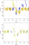 |
Fig. A.1 Light curves of AU Mic b in 2022 (upper panel) and 2023 (lower panel) that were omitted from parameter fitting due to flare complexes during the transits. |
Appendix B Dynamical analyses
Summary of the results of the four dynamical analyses with TRADES. Priors and MAP best-fit solution for each configuration are listed in Table B.1. Observed-Calculated diagrams of the MAP dynamical solution are shown in Fig. B.1, B.2, B.3, and B.4 for configurations (1), (2), (3) and (4), respectively. In Fig. B.5 the RV model from the MAP for the TRADES configuration (4) is shown. Figure B.6 shows the evolution of the projected spin-orbit misalignment (λ RM) of the configuration (2) at synthetic and observed transit times of planet b and c, respectively.
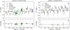 |
Fig. B.1 TRADES modelling of AU Mic b (left panels) and AU Mic c (right panels) of configuration (1). Top panel: (O – C) diagram, observed T0s are plotted with coloured markers with black stroke (different colour and marker for each telescope), while the simulated O – C values computed by the best-fit TRADE S dynamical model are plotted as black line with black circles (corresponding to the observations). Grey-shaded areas correspond to 1, 2, and 3σ of random samples drawn from the posterior distribution of TRADES. Bottom panel: Residuals computed as the difference between observed and simulated T0s. |
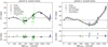 |
Fig. B.2 TRADES modelling of AU Mic b (left panels) and AU Mic c (right panels) of configuration (2). See Fig. B.1 for a description. |
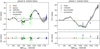 |
Fig. B.3 TRADES modelling of AU Mic b (left panels) and AU Mic c (right panels) of configuration (3). See Fig. B.1 for a description. |
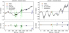 |
Fig. B.4 TRADES modelling of AU Mic b (left panels) and AU Mic c (right panels) of the configuration (4). See Fig. B.1 for a description. |
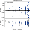 |
Fig. B.5 TRADES RV modelling of AU Mic system of the configuration (4). Black error bars in the lower panel (residuals) take into account the RV jitter term summed in quadrature to the observed uncertainty. |
 |
Fig. B.6 Projected spin-orbit misalignment (λRm) evolution computed at simulated transit during TRADES modelling of AU Mic b (left panels) and AU Mic c (right panels) of configuration (2). Gray circles are all the synthetic transit times, highlighted as black-open circle the corresponding observed transit times. The horizontal-blue line is the mean value of λRm. |
Posterior and derived parameters of the AU Mic system from the four dynamical analyses with TRADES.
References
- Barros, S. C. C., Demangeon, O., Díaz, R. F., et al. 2020, A&A, 634, A75 [EDP Sciences] [Google Scholar]
- Benz, W., Broeg, C., Fortier, A., et al. 2021, Exp. Astron., 51, 109 [Google Scholar]
- Bonfanti, A., Delrez, L., Hooton, M. J., et al. 2021, A&A, 646, A157 [EDP Sciences] [Google Scholar]
- Borsato, L., Marzari, F., Nascimbeni, V., et al. 2014, A&A, 571, A38 [NASA ADS] [CrossRef] [EDP Sciences] [Google Scholar]
- Borsato, L., Malavolta, L., Piotto, G., et al. 2019, MNRAS, 484, 3233 [NASA ADS] [CrossRef] [Google Scholar]
- Borsato, L., Piotto, G., Gandolfi, D., et al. 2021, MNRAS, 506, 3810 [NASA ADS] [CrossRef] [Google Scholar]
- Brandeker, A., Patel, J. A., & Morris, B. M. 2024, PIPE: Extracting PSF photometry from CHEOPS data, Astrophysics Source Code Library [record ascl:2404.002] [Google Scholar]
- Butler, C. J., Byrne, P. B., Andrews, A. D., & Doyle, J. G. 1981, MNRAS, 197, 815 [NASA ADS] [CrossRef] [Google Scholar]
- Cale, B. L., Reefe, M., Plavchan, P., et al. 2021, AJ, 162, 295 [NASA ADS] [CrossRef] [Google Scholar]
- Claret, A. 2021, RNAAS, 5, 13 [NASA ADS] [Google Scholar]
- Deline, A., Queloz, D., Chazelas, B., et al. 2020, A&A, 635, A22 [NASA ADS] [CrossRef] [EDP Sciences] [Google Scholar]
- Delrez, L., Ehrenreich, D., Alibert, Y., et al. 2021, Nat. Astron., 5, 775 [NASA ADS] [CrossRef] [Google Scholar]
- Delrez, L., Leleu, A., Brandeker, A., et al. 2023, A&A, 678, A200 [NASA ADS] [CrossRef] [EDP Sciences] [Google Scholar]
- Donati, J. F., Cristofari, P. I., Finociety, B., et al. 2023, MNRAS, 525, 455 [NASA ADS] [CrossRef] [Google Scholar]
- Foreman-Mackey, D., Hogg, D. W., Lang, D., & Goodman, J. 2013, PASP, 125, 306 [Google Scholar]
- Foreman-Mackey, D., Agol, E., Ambikasaran, S., & Angus, R. 2017, AJ, 154, 220 [Google Scholar]
- Fortier, A., Simon, A. E., Broeg, C., et al. 2024, A&A, 687, A302 [NASA ADS] [CrossRef] [EDP Sciences] [Google Scholar]
- Gaia Collaboration (Vallenari, A., et al.) 2023, A&A, 674, A1 [NASA ADS] [CrossRef] [EDP Sciences] [Google Scholar]
- Gelman, A., & Rubin, D. B. 1992, Statist. Sci., 7, 457 [NASA ADS] [Google Scholar]
- Geweke, J. F. 1991, Evaluating the accuracy of sampling-based approaches to the calculation of posterior moments, Staff Report 148, Federal Reserve Bank of Minneapolis [Google Scholar]
- Gilbert, E. A., Barclay, T., Quintana, E. V., et al. 2022, AJ, 163, 147 [NASA ADS] [CrossRef] [Google Scholar]
- Günther, M. N., & Daylan, T. 2019, Allesfitter: Flexible Star and Exoplanet Inference From Photometry and Radial Velocity, Astrophysics Source Code Library [record ascl:1903.003] [Google Scholar]
- Günther, M. N., & Daylan, T. 2021, ApJS, 254, 13 [CrossRef] [Google Scholar]
- Hebb, L., Petro, L., Ford, H. C., et al. 2007, MNRAS, 379, 63 [CrossRef] [Google Scholar]
- Ilin, E., & Poppenhaeger, K. 2022, MNRAS, 513, 4579 [NASA ADS] [CrossRef] [Google Scholar]
- Kalas, P., Liu, M. C., & Matthews, B. C. 2004, Science, 303, 1990 [Google Scholar]
- Kallinger, T., De Ridder, J., Hekker, S., et al. 2014, A&A, 570, A41 [NASA ADS] [CrossRef] [EDP Sciences] [Google Scholar]
- Kavanagh, R. D., Vidotto, A. A., Klein, B., et al. 2021, MNRAS, 504, 1511 [Google Scholar]
- Kipping, D. M. 2013, MNRAS, 435, 2152 [Google Scholar]
- Kochukhov, O., & Reiners, A. 2020, ApJ, 902, 43 [Google Scholar]
- Lendl, M., Csizmadia, S., Deline, A., et al. 2020, A&A, 643, A94 [EDP Sciences] [Google Scholar]
- MacGregor, M. A., Wilner, D. J., Rosenfeld, K. A., et al. 2013, ApJ, 762, L21 [CrossRef] [Google Scholar]
- Mallorquín, M., Béjar, V. J. S., Lodieu, N., et al. 2024, A&A, 689, A132 [NASA ADS] [CrossRef] [EDP Sciences] [Google Scholar]
- Mamajek, E. E., & Bell, C. P. M. 2014, MNRAS, 445, 2169 [Google Scholar]
- Martioli, E., Hébrard, G., Correia, A. C. M., Laskar, J., & Lecavelier des Etangs, A. 2021, A&A, 649, A177 [NASA ADS] [CrossRef] [EDP Sciences] [Google Scholar]
- Mathioudakis, M., & Doyle, J. G. 1991, A&A, 244, 433 [NASA ADS] [Google Scholar]
- Matthews, B. C., Kennedy, G., Sibthorpe, B., et al. 2015, ApJ, 811, 100 [NASA ADS] [CrossRef] [Google Scholar]
- Nascimbeni, V., Borsato, L., Zingales, T., et al. 2023, A&A, 673, A42 [NASA ADS] [CrossRef] [EDP Sciences] [Google Scholar]
- Nelson, B., Ford, E. B., & Payne, M. J. 2014, ApJS, 210, 11 [Google Scholar]
- Oshagh, M., Santos, N. C., Boisse, I., et al. 2013, A&A, 556, A19 [NASA ADS] [CrossRef] [EDP Sciences] [Google Scholar]
- Parviainen, H., Pallé, E., Nortmann, L., et al. 2016, A&A, 585, A114 [NASA ADS] [CrossRef] [EDP Sciences] [Google Scholar]
- Plavchan, P., Barclay, T., Gagné, J., et al. 2020, Nature, 582, 497 [Google Scholar]
- Schneider, G., Grady, C. A., Hines, D. C., et al. 2014, AJ, 148, 59 [NASA ADS] [CrossRef] [Google Scholar]
- Szabó, G. M., Gandolfi, D., Brandeker, A., et al. 2021, A&A, 654, A159 [NASA ADS] [CrossRef] [EDP Sciences] [Google Scholar]
- Szabó, G. M., Garai, Z., Brandeker, A., et al. 2022, A&A, 659, L7 [NASA ADS] [CrossRef] [EDP Sciences] [Google Scholar]
- ter Braak, C. J. F., & Vrugt, J. A. 2008, Statist. Comput., 18, 435 [NASA ADS] [CrossRef] [Google Scholar]
- Tsikoudi, V., & Kellett, B. J. 2000, MNRAS, 319, 1147 [CrossRef] [Google Scholar]
- Winn, J. N. 2010, in Exoplanets, ed. S. Seager, 55 [Google Scholar]
- Wisniewski, J. P., Kowalski, A. F., Davenport, J. R. A., et al. 2019, ApJ, 883, L8 [Google Scholar]
- Wittrock, J. M., Plavchan, P. P., Cale, B. L., et al. 2023, AJ, 166, 232 [NASA ADS] [CrossRef] [Google Scholar]
- Yu, H., Garai, Z., Cretignier, M., et al. 2025, MNRAS, 536, 2046 [Google Scholar]
- Zicher, N., Barragán, O., Klein, B., et al. 2022, MNRAS, 512, 3060 [NASA ADS] [CrossRef] [Google Scholar]
The mean longitude is defined as λ + ℳ + ω + Ω, where ℳ is the mean anomaly and Ω is the longitude of the ascending node.
We doubled the number of parameter sets/walkers due to the increased number of fitting parameters and the availability of a much more performing server.
In case of all uniform-uninformative priors, the log-probability ln 𝒫 is equal to the log-likelihood ln ℒ.
All Tables
Overview of the Allesfitter priors and best-fitting parameters of AU Mic b and c obtained based on the data from 2022 and 2023.
Overview of the Allesfitter-derived parameters of AU Mic b and c obtained based on the data from 2022 and 2023.
Observed mid-transit times and O – C values of AU Mic b based on TESS, Spitzer, and CHEOPS observations.
Observed mid-transit times and O - C values of AU Mic c based on TESS and CHEOPS observations.
Best-fitting parameters of AU Mic c compared to the results of M2021, G2022, and Sz2022.
Posterior and derived parameters of the AU Mic system from the four dynamical analyses with TRADES.
All Figures
|
Fig. 1 Phased transit light curves of the 2022 and 2023 measurements of the AU Mic b (left panels) and c transits (right panels) after flare removal. The ephemeris and period used here are T0,b = 2458 330.38416d and Pb = 8.4631427d, and T0,c = 2459454.8973 BJD, Pc = 18.85882 d. The TTV is very prominent for both planets compared to the earlier ephemeris. AU Mic b transited after the AU Mic c transit on 22 August 2022 (top right panel), and similarly, planet c transited after planet b on 21 September 2023 (bottom left panel). |
| In the text | |
|
Fig. 2 Stacked and binned CHEOPS transit light curves of AU Mic b (left panels) and AU Mic c (right panels) from 2022 (top panels) and from 2023 (bottom panels), overplotted with the best-fitting Allesfitter models (20 curves from random posterior samples). The residuals are also shown. |
| In the text | |
|
Fig. 3 TTV diagrams of AU Mic b (upper panel) calculated with Tc = 2458 330.38416 and Pmean = 8.4631427 d, and AUMic c (lower panel) calculated with Tc = 2 459 454.8973 and Pmean = 18.85882 d. We included Transiting Exoplanet Survey Satellite (TESS, red symbols), Spitzer (blue symbols), Earth-based Pan-STARRS (light grey symbols) and CHEOPS (black symbols) measurements. The harmonic fit to AU Mic b data (dotted red line) illustrates the most probable shape of a periodic TTV fitted to the data. This is shown to illustrate the trend of the distribution without any dynamical interpretation. |
| In the text | |
|
Fig. A.1 Light curves of AU Mic b in 2022 (upper panel) and 2023 (lower panel) that were omitted from parameter fitting due to flare complexes during the transits. |
| In the text | |
|
Fig. B.1 TRADES modelling of AU Mic b (left panels) and AU Mic c (right panels) of configuration (1). Top panel: (O – C) diagram, observed T0s are plotted with coloured markers with black stroke (different colour and marker for each telescope), while the simulated O – C values computed by the best-fit TRADE S dynamical model are plotted as black line with black circles (corresponding to the observations). Grey-shaded areas correspond to 1, 2, and 3σ of random samples drawn from the posterior distribution of TRADES. Bottom panel: Residuals computed as the difference between observed and simulated T0s. |
| In the text | |
|
Fig. B.2 TRADES modelling of AU Mic b (left panels) and AU Mic c (right panels) of configuration (2). See Fig. B.1 for a description. |
| In the text | |
|
Fig. B.3 TRADES modelling of AU Mic b (left panels) and AU Mic c (right panels) of configuration (3). See Fig. B.1 for a description. |
| In the text | |
|
Fig. B.4 TRADES modelling of AU Mic b (left panels) and AU Mic c (right panels) of the configuration (4). See Fig. B.1 for a description. |
| In the text | |
|
Fig. B.5 TRADES RV modelling of AU Mic system of the configuration (4). Black error bars in the lower panel (residuals) take into account the RV jitter term summed in quadrature to the observed uncertainty. |
| In the text | |
|
Fig. B.6 Projected spin-orbit misalignment (λRm) evolution computed at simulated transit during TRADES modelling of AU Mic b (left panels) and AU Mic c (right panels) of configuration (2). Gray circles are all the synthetic transit times, highlighted as black-open circle the corresponding observed transit times. The horizontal-blue line is the mean value of λRm. |
| In the text | |
Current usage metrics show cumulative count of Article Views (full-text article views including HTML views, PDF and ePub downloads, according to the available data) and Abstracts Views on Vision4Press platform.
Data correspond to usage on the plateform after 2015. The current usage metrics is available 48-96 hours after online publication and is updated daily on week days.
Initial download of the metrics may take a while.