| Issue |
A&A
Volume 694, February 2025
|
|
|---|---|---|
| Article Number | A210 | |
| Number of page(s) | 7 | |
| Section | Planets, planetary systems, and small bodies | |
| DOI | https://doi.org/10.1051/0004-6361/202452563 | |
| Published online | 14 February 2025 | |
GJ 2126 b: A highly eccentric Jovian exoplanet
1
School of Physics and Astronomy, Raymond and Beverly Sackler Faculty of Exact Sciences, Tel Aviv University,
Tel Aviv
6997801,
Israel
2
Porter School of the Environment and Earth Sciences, Raymond and Beverly Sackler Faculty of Exact Sciences, Tel Aviv University,
Tel Aviv
6997801,
Israel
★ Corresponding author; This email address is being protected from spambots. You need JavaScript enabled to view it.
Received:
10
October
2024
Accepted:
28
January
2025
Abstract
We report the discovery of GJ 2126 b, a highly eccentric (e = 0.85) Jupiter-like planet orbiting its host star every 272.7 days. The planet was detected and characterized using 112 radial velocity (RV) measurements from HARPS (High Accuracy Radial velocity Planet Searcher), provided by HARPS-RVBank. This planet orbits a low-mass star and ranks among the most eccentric exoplanets discovered, placing it in a unique region of the parameter space of the known exoplanet population. This makes it a valuable addition to the exoplanet demographics, helping to refine our understanding of planetary formation and evolution theories.
Key words: techniques: radial velocities / planets and satellites: detection / planets and satellites: fundamental parameters / stars: low-mass
© The Authors 2025
 Open Access article, published by EDP Sciences, under the terms of the Creative Commons Attribution License (https://creativecommons.org/licenses/by/4.0), which permits unrestricted use, distribution, and reproduction in any medium, provided the original work is properly cited.
This article is published in open access under the Subscribe to Open model. This email address is being protected from spambots. You need JavaScript enabled to view it. to support open access publication.
1 Introduction
Given the mean eccentricity of e = 0.06 for planets in the Solar System, the discovery of exoplanets with highly eccentric orbits has emerged as one of the most surprising findings in exoplanet research (e.g., O’Toole et al. 2009). Highly eccentric planets exhibit significant variations in their distance from their host stars throughout their orbits, suggesting dynamic histories influenced by diverse gravitational interactions (Booth et al. 2014). This opens up the possibility for various proposed formation and evolution processes (Winn & Fabrycky 2015), such as resonance interaction in the protoplanetary disk (Cresswell et al. 2007), planet-planet scattering (Davies et al. 2014; Carrera et al. 2019), and stellar flybys (Malmberg et al. 2011).
Recent studies indicate that eccentric Jupiters, defined as giant exoplanets with e > 0.25, are abundant, as shown by Buchhave et al. (2018). This conclusion is based on the population characterized following the discovery of the first eccentric Jupiter (16 Cyg Bb; Cochran et al. 1997). However, this does not extend to highly eccentric Jupiters, specifically those with e > 0.6, for which both current models and observations indicate only a limited number (Wittenmyer et al. 2007; Bitsch et al. 2020).
This fact is linked to the unique and dramatic evolutionary path required for such systems to develop (e.g., Wang et al. 2018), believed to occur due to planet–planet gravitational interactions following the gas disc dispersal (Juric & Tremaine 2008; Raymond et al. 2009). Most scenarios that could give rise to such systems would likely lead to moderately eccentric orbits or, conversely, result in the complete ejection of the planet (e.g., Lega et al. 2013).
In this work, we report the detection of an exoplanet occupying this unique parameter space: a highly eccentric Jupiter-like exoplanet, orbiting the low-mass star GJ 2126. The paper is structured as follows: We first discuss the spectroscopic observations of GJ 2126 in Sect. 2. We then describe their analysis in Sect. 3, where we also present the characteristics of the newly detected planet. Finally, we summarize and discuss our findings in Sect. 4.
2 Observations
2.1 HARPS
HARPS (High Accuracy Radial velocity Planet Searcher; Mayor et al. 2003) is a high-resolution visible-light echelle spectrograph installed at the European Southern Observatory (ESO) 3.6-m telescope in La Silla, Chile. With its proven long-term stability and simultaneous calibration it has been demonstrated to reach radial-velocity (RV) accuracy of ∼1 m s−1 (see Pepe et al. 2014).
Despite its high precision, HARPS data are still known to contain minor residual systematics. For instance, Dumusque et al. (2015) identified a one-year variability linked to block stitches in the CCD detector, and a fiber upgrade in May 2015 (Lo Curto et al. 2015) introduced a spectral-type-dependent shift in the RV zero point, of approximately 10 m/s.
Recently, Trifonov et al. (2020) obtained improved and more precise RVs using SERVAL (SpEctrum Radial Velocity AnaLyser; Zechmeister et al. 2018), corrected for HARPS Nightly Zero-Point variations (NZPs; Tal-Or et al. 2019), and made the corrected data publicly available as the HARPS-RVBank dataset. Perdelwitz et al. (2024) later introduced an advanced version, offering enhanced precision and extended temporal coverage. We used measurements from this public dataset for the analysis presented in the following sections.
2.2 Measurements
GJ 2126 is a high proper motion star, and its stellar properties are summarized in Table 1. GJ 2126 was observed by HARPS over a span of 15 years (2004–2019, ~5600 days), with a total of 112 measurements. The measurements, labeled as DRVmlcnzp in Perdelwitz et al. (2024), have an average S/N of 45.0 and a typical RV error of 1.9 m s–1.
Due to the fiber upgrade in May 2015 (Lo Curto et al. 2015), we chose to treat the pre- and post-upgrade RVs as separate data sets from two distinct instruments, each potentially having different zero points (hereafter referred to as “pre-” and “post-”). Of the 112 measurements of GJ 2126, 95 were obtained before the fiber upgrade, while 17 were taken afterward.
In 2020, the observatory was temporarily shut down due to the COVID-19 pandemic1, which introduced an additional offset in the data due to the instrument’s warm-up. As only two further measurements of GJ 2126 were taken after this event, we decided to exclude them from our analysis. No additional data points were omitted.
Although its effective temperature of 4159 ± 129 K suggests it is likely a K-type star, GJ 2126 is commonly referred to in the literature as an M-dwarf (e.g., Kuznetsov et al. 2019; Mignon et al. 2023), a designation that traces back to Stephenson & Sanduleak (1975). While this classification may require reconsideration, it does not affect the results of this paper.
Red dwarfs, of spectral types M and late K, typically exhibit significant stellar activity (see Mignon et al. 2023) due to their convective interiors, which generate strong magnetic fields. This activity can significantly impact RV measurements and, in some cases, even result in false planet detections (e.g., Queloz et al. 2001; Robertson et al. 2014).
To mitigate these effects, we utilized several additional parameters extracted from the cross-correlation function (CCF) of each spectrum, alongside the RVs. These parameters, which are also available in HARPS-RVBank, include the CCF Full-Width at Half-Maximum (FWHM), Contrast, Bisector Inverse Slope (BIS), differential Line Width (dLW) and ChRomatic indeX (CRX) (Zechmeister et al. 2018; Trifonov et al. 2020). Hα and NaD chromospheric line emission (Kürster et al. 2003) are also provided in HARPS-RVBank.
This set of quantities, usually referred to as “activity indicators,” all quantify various aspects of changes in the spectrum shape that can be associated with stellar activity (e.g., Queloz et al. 2001; Gomes da Silva et al. 2011; Dumusque et al. 2011). We used them in our analysis to further establish the orbital nature of the detected signal, as described in the following section. The photometric data available for the target stars, including observations from Hipparcos (Perryman et al. 1997), TESS (Ricker et al. 2015), ASAS-SN (Kochanek et al. 2017), and ZTF (Bellm et al. 2019), were also inspected for transit events, but yielded no noteworthy results.
Stellar parameters of GJ 2126.
3 Analysis
3.1 Periodograms
To initially identify the periodic signal in the measurements, we applied two different periodograms to the RV data: the Generalized Lomb-Scargle periodogram (GLS; Zechmeister & Kürster 2009) and the Phase Distance Correlation periodogram (PDC; Zucker 2018; Binnenfeld et al. 2024).
While the GLS periodogram was selected due to its widespread use, driven by its versatility and computational efficiency, it exhibits an inherent bias toward sinusoidal signals (Pinamonti et al. 2017; Zucker 2018). This bias arises from the fact that the GLS fits a sinusoidal model to the RVs at each trial frequency. The better the model fits the data at a given frequency, the higher the likelihood that the data include a periodic signal at that frequency.
To address this limitation and improve the detection of non- sinusoidal signals, such as those associated with eccentric orbits, we employed the PDC periodogram (Zucker 2018). The PDC periodogram quantifies the statistical dependence between the RV measurements and their phases (according to the trial periods) using the distance correlation dependence measure (Székely et al. 2007). Unlike the GLS periodogram, the PDC periodogram is model-independent, enabling more robust detection of a broader range of signal types, including those arising from eccentric orbits and sawtooth-like pulsation mechanisms.
Figure 1 presents the periodograms for the RVs of GJ 2126. In both periodograms, a prominent peak is visible at the frequency corresponding to a period of —273 days.
Two additional significant peaks, though less prominent, are visible in the periodogram: one at a period of —137 days, which corresponds to a clear harmonic at half the period of the primary peak. The second, at —30 days, is likely an artifact of the lunar cycle. This is supported by the fact that during the years 2004–2012, when most of the RV data were collected, the full moon passed within 15° of the target star for many months.
The periodograms for the various activity indicators provided by HARPS-RVBank (see Sect. 2.2) are presented in Fig. 2. None of the activity indicators showed a peak corresponding to the periods detected in the RV periodogram, making it unlikely that the RV periodicity is related to stellar activity or rotation. A small peak at a period of ~21.5 days seem to be present, mainly in Hα and to a lesser extent in the FWHM, potentially linked to stellar activity or rotation at this frequency (Mignon et al. 2023).
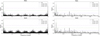 |
Fig. 1 PDC (top left) and GLS (bottom left) periodograms for the RV data. Also shown are the periodograms with a narrower frequency range – PDC (top right) and GLS (bottom right). The horizontal dotted lines indicate the corresponding p-values as noted in the legend. The vertical green dotted line in each periodogram marks the detected period of 273.22 days. |
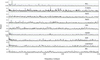 |
Fig. 2 PDC periodograms for the RVs (top) and activity indicators (below). A green vertical line marks the detected planetary period. Blue and green horizontal lines mark the corresponding 10–3 and 10–5 p-values, respectively. |
3.2 Orbital fitting
We fitted a Keplerian orbit to the RVs using Juliet (Espinoza et al. 2019), which employs the radvel code (Fulton et al. 2018) for estimating the parameters of a Keplerian model. The emcee sampler (Foreman-Mackey et al. 2013) available in Juliet was used to perform a Markov Chain Monte Carlo (MCMC) sampling of the posteriors. In addition to the Keplerian elements (P, T0,  ), we fitted a separate offset term for the pre- and post-fiber upgrade datasets (µpre and µpost). We also included an additional white-noise jitter term for each HARPS dataset, denoted by σpre and σpost, to account for any extra noise not captured by the nominal RV error estimates.
To account for potential long-term trends in the data that could indicate the presence of outer companions, we also tested the RVs for a linear slope. The resulting posterior distribution for the slope parameter is consistent with having no slope over the observational baseline, leading us to adopt a model without a linear trend. The lack of a linear trend can provide constraints on the effects of a potential long-period companion, limiting its influence to below the measurement errors over the observation time span. Table 2 presents the priors we used for the MCMC sampling, utilizing a wide range of parameters to ensure comprehensive exploration of the parameter space.
Based on the results of the MCMC run, we derived a best-fit Keplerian model, which is detailed in Table 3 and illustrated in Fig. 3. The keplerian elements e and ω presented in Table 3 were obtained from the fitting parameters  . Figure 4 displays the phase-folded data along with the best-fit model, while Fig. 5 presents the complete corner plot from the MCMC analysis.
We also assessed the periodicity of the model residuals by subtracting the Keplerian solution from the RVs and applying both the PDC and GLS periodograms. No residual signals were detected in this analysis.
Anglada-Escudé et al. (2010) and Wittenmyer et al. (2019) extensively examined the scenario in which a resonant 1:2 two- planet system with circular orbits could be misidentified as a single eccentric planet. To exclude this possibility, we experimented with multi-planetary models during the fitting process, which ultimately ruled out such configurations by providing no viable fit. Furthermore, the sufficient phase coverage, particularly around periastron, combined with the high S/N, further strengthens our confidence in the detection of this eccentric exoplanet. It is also worth noting that, according to current formation models and observational constraints, it is still uncertain whether low-mass stars are likely to host two or more giant planets (see Bryant et al. 2023, for references).
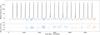 |
Fig. 3 Best-fit Keplerian model for the full RV data (top), and corresponding residuals (bottom). Blue dots represent pre-fiber upgrade measurements, and orange dots represent post-upgrade ones. |
Prior distributions used for the MCMC runs.
Best-fit Keplerian elements for GJ 2126 b.
4 Discussion
In this paper we report the detection and orbital characterization of GJ 2126 b, a highly eccentric (e = 0.85) Jupiter-mass exoplanet orbiting its low-mass host star with a period of 272.7 days. Its unique properties place it in a relatively sparse region of the detected exoplanet population, offering valuable insights for current planetary formation and evolution models.
As discussed in Sect. 2.2, GJ 2126, is widely referred to in the literature as an M-dwarf star. Only a relatively small number of eccentric exoplanets have been detected around M-dwarf stars, despite their importance for various open questions. These include dynamically unexplained cases of high eccentricities in systems where circularization was expected (e.g., Stevenson et al. 2014), and correlations between eccentricities and various stellar parameters (see Sagear & Ballard 2023). Another key question is the habitability of M-dwarf star systems, where tidal heating caused by high eccentricity is expected to eliminate the possibility of life-supporting conditions (Barnes et al. 2013). This discovery contributes a valuable piece of data to this exoplanet demographics and it can be used to refine observing strategies and models (e.g., Sabotta et al. 2021).
With its inclination remaining unknown, it could be argued that the detected companion is significantly more massive than the suggested 1.3 MJ and in fact not planetary in its nature. For the companion to be classified within the brown dwarf regime, its orbital orientation would need to be nearly face-on (i ≲ 6°). This is highly unlikely given the distribution of observed inclinations (e.g., Bertaux & Ivanova 2022, and references therein).
Furthermore, we ruled out this possibility based on astrometric measurements from both Hipparcos and Gaia, which exclude the existence of such a massive companion (Kervella et al. 2019, 2022). Additionally, the Renormalized Unit Weight Error (RUWE) value for the star from Gaia third Data Release (DR3) is approximately one, strongly indicating the absence of an astrometric signal of a massive companion (Gaia Collaboration 2023a; Babusiaux et al. 2023). Given the characteristics of GJ 2126 b, the detection of such a companion should have been well within Gaia capabilities (Perryman et al. 2014; Sozzetti et al. 2014).
The reported exoplanet calls for an explanation that can account for its high eccentricity. Since planets are assumed to form within protoplanetary disks, their initial orbits should have been circular or close to circular, as the disk gaseous viscosity tends to dampen any orbital eccentricity (e.g., Bitsch et al. 2013). Gravitational interactions between planets and the disk, where eccentricity increases due to significant gaps in the disk (Papaloizou et al. 2001), are only relevant for the eccentricity of very massive planets exceeding five Jupiter masses (Kley & Dirksen 2006).
The Lidov–Kozai effect (Mazeh & Shaham 1979; Naoz 2016) is a potential mechanism that could account for the observed eccentricity by inducing oscillations in the orbit inclination and eccentricity through gravitational interactions with an additional, long-period massive companion in the system. However, as discussed earlier, astrometric measurements from Hipparcos and Gaia rule out the existence of such a companion, excluding this possibility. The absence of a long-term trend in the data, discussed in Sect. 3.2, further supports this conclusion.
A scattering event induced by a stellar flyby also seems unlikely due to the relatively close-in orbit of the planet. As demonstrated by Zakamska & Tremaine (2004), a stellar flyby with an impact parameter of several hundred Astronomical Units (AU) could significantly affect planets with longer-period orbits (a ≥ 50 AU). However, planets with shorter orbits would not experience substantial perturbations from such encounters (Bancelin et al. 2019). While closer flybys might occur during early evolution stages within a star cluster, the resulting eccentricity of the planets would likely be damped over time by the surrounding protoplanetary disk (Picogna & Marzari 2014).
The most likely explanation we propose for the observed high eccentricity is scattering through planet-planet interactions. Recent simulations indicate that such interactions can lead to extreme eccentricity values (Carrera et al. 2019). Specifically, this process involves multiple young planets with moderate eccentricities forming in suitable locations and interacting with one another. As some planets are ejected from the system, angular momentum transfer can increase the remaining planets eccentricities (Wang et al. 2018). Ford & Rasio (2008) demonstrated that these scattering events are most effective when the interacting planets have comparable masses, which provides further insight into the potential evolutionary history of GJ 2126. It is also plausible that the described process is part of high-eccentricity tidal migration, an evolutionary pathway that may explain the origins of hot Jupiters (see Dawson & Johnson 2018).
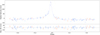 |
Fig. 4 The RVs phase-folded according to the best-fit Keplerian model (top), and the corresponding residuals (bottom). Blue dots represent prefiber upgrade measurements, and orange dots represent post-upgrade ones. |
 |
Fig. 5 Corner plot for the best-fit parameters. |
Acknowledgements
We are grateful to the anonymous referee for their insightful comments, which helped improve the manuscript. This research was supported by the ISRAEL SCIENCE FOUNDATION (grant No. 1404/22) and the Israel Ministry of Science and Technology (grant No. 3-18143). This work has made use of data from the European Space Agency (ESA) mission Gaia (https://www.cosmos.esa.int/gaia), processed by the Gaia Data Processing and Analysis Consortium (DPAC, https://www.cosmos.esa.int/web/gaia/dpac/consortium). Funding for the DPAC has been provided by national institutions, in particular the institutions participating in the Gaia Multilateral Agreement. The analyses done for this paper made use of the code packages: NumPy (Harris et al. 2020), SciPy (Virtanen et al. 2020), Juliet (Espinoza et al. 2019), radvel (Fulton et al. 2018) and SPARTA (Shahaf et al. 2020)2.
References
- Anglada-Escudé, G., López-Morales, M., & Chambers, J. E. 2010, ApJ, 709, 168 [CrossRef] [Google Scholar]
- Babusiaux, C., Fabricius, C., Khanna, S., et al. 2023, A&A, 674, A32 [NASA ADS] [CrossRef] [EDP Sciences] [Google Scholar]
- Bancelin, D., Nordlander, T., Pilat-Lohinger, E., & Loibnegger, B. 2019, MNRAS, 486, 4773 [CrossRef] [Google Scholar]
- Barnes, R., Mullins, K., Goldblatt, C., et al. 2013, Astrobiology, 13, 225 [Google Scholar]
- Bellm, E. C., Kulkarni, S. R., Graham, M. J., et al. 2019, PASP, 131, 018002 [Google Scholar]
- Bertaux, J.-L., & Ivanova, A. 2022, MNRAS, 512, 5552 [NASA ADS] [CrossRef] [Google Scholar]
- Binnenfeld, A., Shahaf, S., & Zucker, S. 2024, A&A, 686, A192 [NASA ADS] [CrossRef] [EDP Sciences] [Google Scholar]
- Bitsch, B., Crida, A., Libert, A. S., & Lega, E. 2013, A&A, 555, A124 [NASA ADS] [CrossRef] [EDP Sciences] [Google Scholar]
- Bitsch, B., Trifonov, T., & Izidoro, A. 2020, A&A, 643, A66 [EDP Sciences] [Google Scholar]
- Booth, M., Matthews, B. C., & Graham, J. R., eds. 2014, IAU Symposium, 299, Exploring the Formation and Evolution of Planetary Systems [Google Scholar]
- Bryant, E. M., Bayliss, D., & Van Eylen, V. 2023, MNRAS, 521, 3663 [CrossRef] [Google Scholar]
- Buchhave, L. A., Bitsch, B., Johansen, A., et al. 2018, ApJ, 856, 37 [Google Scholar]
- Carrera, D., Raymond, S. N., & Davies, M. B. 2019, A&A, 629, L7 [NASA ADS] [CrossRef] [EDP Sciences] [Google Scholar]
- Cochran, W. D., Hatzes, A. P., Butler, R. P., & Marcy, G. W. 1997, ApJ, 483, 457 [Google Scholar]
- Cresswell, P., Dirksen, G., Kley, W., & Nelson, R. P. 2007, A&A, 473, 329 [NASA ADS] [CrossRef] [EDP Sciences] [Google Scholar]
- Davies, M. B., Adams, F. C., Armitage, P., et al. 2014, in Protostars and Planets VI, eds. H. Beuther, R. S. Klessen, C. P. Dullemond, & T. Henning, 787 [Google Scholar]
- Dawson, R. I., & Johnson, J. A. 2018, ARA&A, 56, 175 [Google Scholar]
- Dumusque, X., Lovis, C., Ségransan, D., et al. 2011, A&A, 535, A55 [NASA ADS] [CrossRef] [EDP Sciences] [Google Scholar]
- Dumusque, X., Pepe, F., Lovis, C., & Latham, D. W. 2015, ApJ, 808, 171 [NASA ADS] [CrossRef] [Google Scholar]
- Espinoza, N., Kossakowski, D., & Brahm, R. 2019, MNRAS, 490, 2262 [Google Scholar]
- Ford, E. B., & Rasio, F. A. 2008, ApJ, 686, 621 [Google Scholar]
- Foreman-Mackey, D., Hogg, D. W., Lang, D., & Goodman, J. 2013, PASP, 125, 306 [Google Scholar]
- Fulton, B. J., Petigura, E. A., Blunt, S., & Sinukoff, E. 2018, PASP, 130, 044504 [Google Scholar]
- Gaia Collaboration (Prusti, T., et al.) 2016, A&A, 595, A1 [NASA ADS] [CrossRef] [EDP Sciences] [Google Scholar]
- Gaia Collaboration (Arenou, F., et al.) 2023a, A&A, 674, A34 [CrossRef] [EDP Sciences] [Google Scholar]
- Gaia Collaboration (Vallenari, A., et al.) 2023b, A&A, 674, A1 [NASA ADS] [CrossRef] [EDP Sciences] [Google Scholar]
- Gomes da Silva, J., Santos, N. C., Bonfils, X., et al. 2011, A&A, 534, A30 [NASA ADS] [CrossRef] [EDP Sciences] [Google Scholar]
- Harris, C. R., Millman, K. J., van der Walt, S. J., et al. 2020, Nature, 585, 357 [NASA ADS] [CrossRef] [Google Scholar]
- Juric, M., & Tremaine, S. 2008, ApJ, 686, 603 [NASA ADS] [CrossRef] [Google Scholar]
- Kervella, P., Arenou, F., Mignard, F., & Thévenin, F. 2019, A&A, 623, A72 [NASA ADS] [CrossRef] [EDP Sciences] [Google Scholar]
- Kervella, P., Arenou, F., & Thévenin, F. 2022, A&A, 657, A7 [NASA ADS] [CrossRef] [EDP Sciences] [Google Scholar]
- Kley, W., & Dirksen, G. 2006, A&A, 447, 369 [NASA ADS] [CrossRef] [EDP Sciences] [Google Scholar]
- Kochanek, C. S., Shappee, B. J., Stanek, K. Z., et al. 2017, PASP, 129, 104502 [Google Scholar]
- Kürster, M., Endl, M., Rouesnel, F., et al. 2003, A&A, 403, 1077 [NASA ADS] [CrossRef] [EDP Sciences] [Google Scholar]
- Kuznetsov, M. K., del Burgo, C., Pavlenko, Y. V., & Frith, J. 2019, ApJ, 878, 134 [Google Scholar]
- Lega, E., Morbidelli, A., & Nesvorný, D. 2013, MNRAS, 431, 3494 [NASA ADS] [CrossRef] [Google Scholar]
- Lo Curto, G., Pepe, F., Avila, G., et al. 2015, The Messenger, 162, 9 [NASA ADS] [Google Scholar]
- Malmberg, D., Davies, M. B., & Heggie, D. C. 2011, MNRAS, 411, 859 [Google Scholar]
- Mayor, M., Pepe, F., Queloz, D., et al. 2003, The Messenger, 114, 20 [NASA ADS] [Google Scholar]
- Mazeh, T., & Shaham, J. 1979, A&A, 77, 145 [Google Scholar]
- Mignon, L., Meunier, N., Delfosse, X., et al. 2023, A&A, 675, A168 [NASA ADS] [CrossRef] [EDP Sciences] [Google Scholar]
- Naoz, S. 2016, ARA&A, 54, 441 [Google Scholar]
- O’Toole, S. J., Tinney, C. G., Jones, H. R. A., et al. 2009, MNRAS, 392, 641 [Google Scholar]
- Papaloizou, J. C. B., Nelson, R. P., & Masset, F. 2001, A&A, 366, 263 [NASA ADS] [CrossRef] [EDP Sciences] [Google Scholar]
- Pepe, F., Ehrenreich, D., & Meyer, M. R. 2014, Nature, 513, 358 [NASA ADS] [CrossRef] [Google Scholar]
- Perdelwitz, V., Trifonov, T., Teklu, J. T., Sreenivas, K. R., & Tal-Or, L. 2024, A&A, 683, A125 [NASA ADS] [CrossRef] [EDP Sciences] [Google Scholar]
- Perryman, M. A. C., Lindegren, L., Kovalevsky, J., et al. 1997, A&A, 323, L49 [Google Scholar]
- Perryman, M., Hartman, J., Bakos, G. Á., & Lindegren, L. 2014, ApJ, 797, 14 [Google Scholar]
- Picogna, G., & Marzari, F. 2014, A&A, 564, A28 [NASA ADS] [CrossRef] [EDP Sciences] [Google Scholar]
- Pinamonti, M., Sozzetti, A., Bonomo, A. S., & Damasso, M. 2017, MNRAS, 468, 3775 [CrossRef] [Google Scholar]
- Queloz, D., Henry, G. W., Sivan, J. P., et al. 2001, A&A, 379, 279 [NASA ADS] [CrossRef] [EDP Sciences] [Google Scholar]
- Raymond, S. N., Armitage, P. J., & Gorelick, N. 2009, ApJ, 699, L88 [Google Scholar]
- Ricker, G. R., Winn, J. N., Vanderspek, R., et al. 2015, J. Astron. Telesc. Instrum. Syst., 1, 014003 [Google Scholar]
- Robertson, P., Mahadevan, S., Endl, M., & Roy, A. 2014, Science, 345, 440 [Google Scholar]
- Sabotta, S., Schlecker, M., Chaturvedi, P., et al. 2021, A&A, 653, A114 [NASA ADS] [CrossRef] [EDP Sciences] [Google Scholar]
- Sagear, S., & Ballard, S. 2023, Proc. Natl. Acad. Sci. U.S.A., 120, e2217398120 [NASA ADS] [CrossRef] [Google Scholar]
- Shahaf, S., Binnenfeld, A., Mazeh, T., & Zucker, S. 2020, Astrophysics Source Code Library [record ascl:2007.022] [Google Scholar]
- Sozzetti, A., Giacobbe, P., Lattanzi, M. G., et al. 2014, MNRAS, 437, 497 [NASA ADS] [CrossRef] [Google Scholar]
- Stassun, K. G., Oelkers, R. J., Paegert, M., et al. 2019, AJ, 158, 138 [Google Scholar]
- Stephenson, C. B., & Sanduleak, N. 1975, AJ, 80, 972 [NASA ADS] [CrossRef] [Google Scholar]
- Stevenson, K. B., Bean, J. L., Fabrycky, D., & Kreidberg, L. 2014, ApJ, 796, 32 [NASA ADS] [CrossRef] [Google Scholar]
- Székely, G. J., Rizzo, M. L., & Bakirov, N. K. 2007, Ann. Stat., 35, 2769 [Google Scholar]
- Tal-Or, L., Trifonov, T., Zucker, S., Mazeh, T., & Zechmeister, M. 2019, MNRAS, 484, L8 [Google Scholar]
- Trifonov, T., Tal-Or, L., Zechmeister, M., et al. 2020, A&A, 636, A74 [NASA ADS] [CrossRef] [EDP Sciences] [Google Scholar]
- Virtanen, P., Gommers, R., Oliphant, T. E., et al. 2020, Nat. Methods, 17, 261 [Google Scholar]
- Wang, J. J., Graham, J. R., Dawson, R., et al. 2018, AJ, 156, 192 [Google Scholar]
- Winn, J. N., & Fabrycky, D. C. 2015, ARA&A, 53, 409 [Google Scholar]
- Wittenmyer, R. A., Endl, M., Cochran, W. D., & Levison, H. F. 2007, AJ, 134, 1276 [NASA ADS] [CrossRef] [Google Scholar]
- Wittenmyer, R. A., Bergmann, C., Horner, J., Clark, J., & Kane, S. R. 2019, MNRAS, 484, 4230 [NASA ADS] [CrossRef] [Google Scholar]
- Zakamska, N. L., & Tremaine, S. 2004, AJ, 128, 869 [NASA ADS] [CrossRef] [Google Scholar]
- Zechmeister, M., & Kürster, M. 2009, A&A, 496, 577 [CrossRef] [EDP Sciences] [Google Scholar]
- Zechmeister, M., Reiners, A., Amado, P. J., et al. 2018, A&A, 609, A12 [NASA ADS] [CrossRef] [EDP Sciences] [Google Scholar]
- Zucker, S. 2018, MNRAS, 474, L86 [NASA ADS] [CrossRef] [Google Scholar]
Nov. 9, 2020 entry; https://www.eso.org/sci/facilities/lasilla/instruments/harps/news.html
All Tables
All Figures
|
Fig. 1 PDC (top left) and GLS (bottom left) periodograms for the RV data. Also shown are the periodograms with a narrower frequency range – PDC (top right) and GLS (bottom right). The horizontal dotted lines indicate the corresponding p-values as noted in the legend. The vertical green dotted line in each periodogram marks the detected period of 273.22 days. |
| In the text | |
|
Fig. 2 PDC periodograms for the RVs (top) and activity indicators (below). A green vertical line marks the detected planetary period. Blue and green horizontal lines mark the corresponding 10–3 and 10–5 p-values, respectively. |
| In the text | |
|
Fig. 3 Best-fit Keplerian model for the full RV data (top), and corresponding residuals (bottom). Blue dots represent pre-fiber upgrade measurements, and orange dots represent post-upgrade ones. |
| In the text | |
|
Fig. 4 The RVs phase-folded according to the best-fit Keplerian model (top), and the corresponding residuals (bottom). Blue dots represent prefiber upgrade measurements, and orange dots represent post-upgrade ones. |
| In the text | |
|
Fig. 5 Corner plot for the best-fit parameters. |
| In the text | |
Current usage metrics show cumulative count of Article Views (full-text article views including HTML views, PDF and ePub downloads, according to the available data) and Abstracts Views on Vision4Press platform.
Data correspond to usage on the plateform after 2015. The current usage metrics is available 48-96 hours after online publication and is updated daily on week days.
Initial download of the metrics may take a while.