| Issue |
A&A
Volume 694, February 2025
|
|
|---|---|---|
| Article Number | A157 | |
| Number of page(s) | 11 | |
| Section | Catalogs and data | |
| DOI | https://doi.org/10.1051/0004-6361/202452042 | |
| Published online | 11 February 2025 | |
Stellar magnetic activity in Earth 2.0 candidates based on LAMOST DR10
1
College of Physics, Guizhou University,
550025
Guiyang,
PR China
2
Dept. of Physics and Astronomy and SARA, Butler University,
Indianapolis,
IN
46208,
USA
3
Department of Physics & Astronomy Howard University,
Washington,
DC
20059,
USA
4
College of big data and information engineering, Guizhou University,
550025
Guiyang,
PR China
5
College of medicine, Guizhou university of traditional Chinese medicine,
Guiyang
550025,
PR China
★ Corresponding authors; This email address is being protected from spambots. You need JavaScript enabled to view it.
; This email address is being protected from spambots. You need JavaScript enabled to view it.
Received:
29
August
2024
Accepted:
23
December
2024
Abstract
Aims. Stellar chromospheric activity can impact the search for exoplanets. Earth 2.0 (ET 2.0) is a space telescope designed for exoplanet detection. In this work, we survey the stellar chromospheric activity in the ET 2.0 target regions to enhance the detection rate of exoplanets.
Methods. This work uses Hα and Ca II H&K lines as indicators of chromospheric activity and conducts a survey of stellar chromospheric activity in the ET 2.0 target regions using LAMOST low- and medium-resolution spectra. After cross-referencing with the ET 2.0 input catalog, we obtained over 349 000 low-resolution spectra and over 30 000 medium-resolution spectra from LAMOST. We quantified the chromospheric activity intensity for all spectra and selected the results for those with a signal-to-noise ratio (S/N) above 10 for further studies of the chromospheric activity. The quantification standards include equivalent width (EW) and the ratio of bolometric luminosity to the corresponding spectral line luminosity (LHα/Lbol, LCaH/Lbol, LCaK/Lbol, LHK/Lbol).
Results. Utilizing Hα and Ca II H&K lines, we evaluated the chromospheric activity for over 320 000 and 110 000 spectra based on LAMOST low-resolution spectra, respectively. In addition, we evaluated chromospheric activity for 34000 spectra using Hα lines based on medium-resolution spectra. We selected samples that are suitable for exoplanet studies, based on Hα and Ca II H&K lines. Additionally, we explored the relationship between stellar activity observed by LAMOST and rotation periods obtained from Kepler and TESS surveys. Our findings confirm the presence of two distinct regions in terms of their relationship between stellar activity and Rossby number (Ro), namely: saturated and unsaturated. We determined a critical Ro in the range of 0.09–0.12 using the r-band spectra of 11 921 stars and u-band spectra of 6120 stars. Moreover, we observe that Ca II H&K lines exhibit greater sensitivity to Ro in the unsaturated region, compared to Ha line measurements. Lastly, we have established positive correlations between various activity indicators, including R′CaK, R′CaH, R′HK, and R′Hα.
Key words: catalogs / surveys / stars: activity / stars: chromospheres
© The Authors 2025
 Open Access article, published by EDP Sciences, under the terms of the Creative Commons Attribution License (https://creativecommons.org/licenses/by/4.0), which permits unrestricted use, distribution, and reproduction in any medium, provided the original work is properly cited.
This article is published in open access under the Subscribe to Open model. This email address is being protected from spambots. You need JavaScript enabled to view it. to support open access publication.
1 Introduction
The discovery of planets around PSR 1257+12 by Wolszczan & Frail (1992), utilizing pulsar timing, marked a pivotal moment in astrophysics, offering the first confirmation of exoplanetary existence beyond our Solar System. Subsequently, Mayor & Queloz (1995) achieved a groundbreaking milestone by detecting a Jupiter-mass exoplanet orbiting 51 Pegasi, ushering in a new era of exoplanet exploration around solar-like stars. Over recent years, advancements in projects such as Kepler (Koch et al. 2010), Transiting Exoplanet Survey Satellite (TESS, Ricker et al. 2014), and the High Accuracy Radial Velocity Planet Search (HARPS, Mayor et al. 2003) have exponentially increased the tally of exoplanet discoveries. Currently, China is developing the ET 2.0 space telescope, specifically designed to hunt for exoplanets, with a primary focus on Sun-like stars in search of habitable Earth-like planets (Ge et al. 2022). Stellar activity plays a crucial role not only in shaping space weather and impacting daily life (Lingam & Loeb 2017; Linsky et al. 2019; Tu et al. 2020) but also in modulating planetary atmospheres, thereby influencing a planet’s habitability (Thomas et al. 2007; Kay et al. 2016; Su et al. 2022). As such, understanding stellar activity is vital for comprehending both cosmic phenomena and the potential habitability of distant worlds.
Stellar activity manifests itself through a plethora of phenomena, including flares (Hawley et al. 2014), spots (Berdyugina 2005; Strassmeier 2009), and coronal mass ejections (CMEs, Antiochos et al. 1999; Lu et al. 2022), among others. These phenomena are intricately linked to stellar magnetic activity and internal dynamo processes (Parker 1955; Babcock 1958; Leighton 1969; Middelkoop 1982). Chromospheric activity indicators encompass a range of spectral lines such as Na I D1, D2, Ca II infrared triplet (IRT), Hα, Hβ, Ca II H&K, He I D3 , and more (Montes et al. 1997; Gunn & Doyle 1997). Notably, the Ca II H&K lines (Mamajek & Hillenbrand 2008; Browning et al. 2010; Zhao et al. 2013; Zhang et al. 2020) and the Hα line (Delfosse et al. 1998; Mohanty & Basri 2003; Long et al. 2021) stand out as the most widely utilized chromospheric activity indicators. Recent years have witnessed a surge in studies on stellar activity leveraging large-scale stellar datasets (Frasca et al. 2016; Zhang et al. 2018; Long et al. 2021). Researchers have tapped into data from the Sloan Digital Sky Survey (SDSS) (York et al. 2000) and LAMOST (Cui et al. 2012) to unravel the intricate relationships between stellar activity, rotation periods, and age. Concurrently, the integration of photometric data from Kepler and the TESS survey has enabled analyses of the interplay between chromospheric activity, flares, and spots (Lu et al. 2019; Zhang et al. 2020; Tu et al. 2021; Zhang et al. 2023). These investigations consistently highlight that stars exhibiting heightened chromospheric activity tend to experience more frequent and intense flares, larger sunspots, and shorter rotation periods.
Wilson (1963, 1968) pioneered the study of stellar chromospheric activity by focusing on the Ca II H&K lines. They introduced the S-index as a metric to quantify the intensity of Ca II H&K lines, establishing its efficacy in evaluating chromospheric activity among main-sequence stars. Defined as the ratio of the line-center flux of the Ca II H&K lines to the adjacent continuum spectrum (Vaughan et al. 1978). Building upon Wilson’s work, Vaughan & Preston (1980) investigated the activity levels of nearby stars using the Ca II H&K lines, revealing a correlation between stellar spectral types and activity levels, with solar-like stars typically exhibiting weaker activity. Middelkoop (1982) further refined the analysis by converting the emission indices of Ca II H&K lines into surface flux near the H and K lines, mitigating the dependence of Ca II H&K emission intensity on spectral characteristics. Noyes et al. (1984) introduced the chromospheric emission parameter  , which (through an empirical formula) effectively isolated chromospheric activity from photospheric contributions; thus, the accuracy of Ca II H&K emission index measurements could be enhanced, while minimizing the influence of spectral type and effective temperature (Teff ). Herbig (1985) extended the exploration of chromospheric activity indicators to F8-G3 type main sequence stars, highlighting the utility of the Hα line in assessing activity levels for these stars. Stauffer & Hartmann (1986) analyzed the Hα line of approximately 1000 M-dwarf stars and studied their chromospheric activity. In a more recent development, Fang et al. (2018) introduced parameters
  and
and  akin to
  , aimed at mitigating the influence of stellar spectral type and (Teff ) on the assessment of Hα and Hβ line activity. These advancements have significantly contributed to our understanding of stellar chromospheric activity across various spectral types.
The chromospheric activity intensity is influenced not only by the (Teff ), but also by stellar rotation (Stauffer & Hartmann 1987; Schrijver et al. 1989). Kraft (1967) was among the first to establish a strong positive correlation between stellar rotation and chromospheric activity intensity. Building on this, Noyes et al. (1984) identified a robust relationship between chromospheric activity and the ratio of the stellar rotation period to the convective overturn timescale, known as the Ro. Further insights were gleaned by Reiners et al. (2009), who utilized the Hα line and X-ray intensity to uncover that the saturation state of magnetic flux is consistent across both the corona and chromospheric emission, with a critical Ro of approximately 0.1. Subsequent research has delved into determining critical Ro Douglas et al. (2014); Newton et al. (2017); Fang et al. (2018) with findings that consistently fall within the range of 0.1–0.3. However, a definitive determination of this critical value requires ongoing discussion and investigation.
The primary scientific objective of ET 2.0 is to detect habitable exoplanets using the transit method. The primary scientific objective of ET 2.0 is to search for habitable exoplanets using the transit method. However, stellar magnetic activity introduces noise into exoplanet transits (Ballerini et al. 2012; Zhang et al. 2024). Furthermore, stellar activity significantly affects the habitability of exoplanets. The next section introduces our data sample, followed by an analysis of the activity properties of the Hα line and the Ca II H&K lines in Sect. 3, where we also determine the relationship between chromospheric activity and stellar parameters. Finally, we provide a summary of our findings in Sect. 4.
2 Data analysis
2.1 ET 2.0
ET 2.0 represents a cutting-edge space telescope that is currently in the developmental stages in China. Its configuration comprises six 30 centimeter (cm) transit telescopes alongside one microlensing telescope. These telescopes operate within a wavelength range of 450–900 nanometre (nm). Its photometric precision is approximately 34 ppm/6.5 h. The microlensing telescope, adopting the Schmidt-Mann catadioptric system, operates within a narrower wavelength span of 700–900 nm. The observation strategy of ET 2.0 is to position itself at the center of the Kepler field of view, observing a square region centered at RA=290.67°, Dec=44.5°, with a side length of 22.36 degrees. Candidate stars for observation are meticulously selected from the Caia DR3 database (Gaia Collaboration 2021, 2023), with a preference for those with G-magnitudes brighter than 16. The main observational targets of ET 2.0 are Sun-like stars, with spectral types ranging from K5 to F5. However, in pursuit of detecting smaller exoplanets similar in size to Earth, ET 2.0 strategically directs its observations toward dwarf stars, particularly those with radii less than 2.5 times that of the Sun (Ge et al. 2022). Based on the above observational requirements, ET 2.0 will focus on stars with spectral types ranging from M9 to F5. This targeted approach underscores the necessity of pinpointing host stars with minimal activity-induced noise to optimize the detection potential of ET 2.0 for Earth-sized planets.
2.2 LAMOST spectra
Installed at the Xinglong Observatory in China, LAMOST comprises a reflective Schmidt corrector plate (MA) and a spherical primary mirror (MB). With an effective aperture of 4 m and a field of view diameter spanning 5 degrees, LAMOST can simultaneously observe 4000 stars and acquire their spectral data (Wang et al. 1996; Cui et al. 2012; Zhao et al. 2012). To date, LAMOST has amassed over ten million low-resolution spectra (R~1800), alongside a commensurate number of mediumresolution spectra (R~7500). The wavelength coverage of the low-resolution observation mode spans 370–900 nm (Luo et al. 2015), while the medium-resolution observation mode is divided into two parts: one covering 495–535 nm, and the other covering 630–680 nm (Liu et al. 2020). Since the input star catalog for ET 2.0 is based on Gaia DR3, we first identified all Gaia DR3 sources within the ET 2.0 field. Subsequently, we cross-matched this catalog with LAMOST DR10 low-resolution spectra, employing a matching criterion of 2 arcseconds for source alignment. In cases where multiple results were within 2 arcseconds, the brighter star was prioritized as the LAM- OST spectral observation result. Using this methodology, we extracted more than 349 000 spectra from the LAMOST low- resolution survey and over 30 000 spectra from the LAMOST medium-resolution survey. We employed Gaia DR3 data to construct the Hertzsprung–Russell diagram (HRD), visualized in the leftmost panel of the first row of Figure 1. The subsequent analysis involved utilizing the atmospheric parameters provided by LAMOST DR10 ((Teff), log 𝑔, [Fe/H]) to generate two additional plots of physical parameters, as depicted in Figure 1. In the middle set of panels in Figure 1, we used the empirical relationship between (Teff), log 𝑔, and spectral types proposed by Ciardi et al. (2011), represented by a black dashed line, to classify the sample into main sequence stars and giants. The specific formula is as follows:
 (1)
(1)
Due to the exclusion of giant stars as observation targets for ET 2.0, this study predominantly centers its investigation on the chromospheric activity of main sequence stars.
The low-resolution survey conducted by LAMOST encompasses five bands: u, g, r, z, and i. In this study, our analysis primarily revolves around the Ca II H&K lines and the Hα line for probing stellar chromospheric activity. We quantified the chromospheric activity for all spectra. However, to ensure the reliability of the results in our statistical analysis, we applied a selection criterion based on the signal-to-noise ratio (S/N) of the spectra. The wavelengths of the Ca II H&K lines are 3933 Å and 3968 Å, corresponding to the u band of the LAMOST spectrum. Thus, our selection criteria for discussing Ca II H&K lines entail opting for spectra with a S/N greater than 10 in the u band. Similarly, the central wavelength of the Hα line is 6562.8 Å, aligning with the r band of the LAMOST spectrum. Consequently, we opted for spectra with S/N greater than 10 in the r band to examine the Hα line. When simultaneously addressing both Ca II H&K lines and the Hα line, we utilize spectra with S/N greater than 10 in both the u and r bands. The S/N distribution of the samples analyzed in this study is depicted in Figure 2. The panels on the left side of Fig. 2 show the S/N statistics for the low-resolution data, while the panels on the right side represent the S/N statistics for the medium-resolution data.
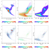 |
Fig. 1 LAMOST DR10 low-resolution and medium-resolution samples in the ET 2.0 field, presented in the three panels above and the three panels below, respectively. The left, middle, and right panels of each set of images represent the relationship diagrams of different physical parameters. Left panel: HRD based on Gaia DR3 data. The color bar indicates the number density of stars. Middle panel: The relationship diagram between (Teff) and log 𝑔 based on LAMOST DR10 data, with the color bar representing the parameter [Fe/H]. The black dashed line represents the empirical formula proposed by Ciardi et al. (2011). Dividing the samples into giant stars (above the line) and main-sequence stars (below the line). Right panel: relationship diagram between (Teff) and log g based on LAMOST DR10 data, with the color bar indicating the number density of stars. |
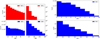 |
Fig. 2 S/N distribution statistics for the u and r bands of the low-resolution data (left panels). S/N distribution statistics for the r band of the medium-resolution data (right panels). |
3 Chromospheric activity
3.1 Hα
3.1.1 EW of Hα
The Hα line stands as a widely acknowledged indicator of stellar chromospheric activity (West et al. 2008; Newton et al. 2017). In particular, for low-mass stars, the S/N near the Ca II H&K lines is often insufficient. This deficiency is evident in our statistical analysis of S/N, as illustrated in Figure 2. Since our sample includes low-mass stars, analyzing the Hα spectral line is essential. Notably, our analysis reveals fewer than 110 000 spectra with S/N greater than 10 in the u band, whereas over 320 000 spectra boast S/N exceeding 10 in the r band. Therefore, for LAMOST data, the red-band spectrum near the Hα line has better quality, allowing us to conduct research on chromospheric activity using the Hα line. The equivalent width (EW) of Hα serves as a commonly employed parameter for quantifying the Hα line (Montes et al. 1995; Zhang et al. 2021). In this study, we also calculated the EW of Hα as one of the key indicators for assessing the Hα line. We employed the following formula, as outlined by (Hawley et al. 2002; West et al. 2004):
 (2)
(2)
Here, Fλ and Fc represent the spectral line flux and the continuum flux, respectively. Also, Fc is derived from the median of the continuous spectrum range after resampling the normalized spectrum. Based on this formula, when the obtained EW value is greater than or equal to 0, it indicates that the Hα line of the spectrum is an emission line. Conversely, when the EW is less than 0, it indicates that the Hα line of the corresponding spectrum is an absorption line. The selection of spectral line ranges and continuum ranges often requires different approaches. Furthermore, the choice of range significantly impacts our calculation of the Hα EW results. For instance, Zhang et al. (2016) chose a range of 4 Å at each end of the line center as the calculation area for Fλ, focusing primarily on M dwarfs. Conversely, Fang et al. (2018) employed a range of 6557–6569 Å and studied stars below 6500 K. Notably, the linewidth of the Hα line decreases as the (Teff) of the star increases (Mihalas 1978). Therefore, for F-type stars, a wider range of the Hα line is warranted. Our sample, as depicted in the Figure 1, comprises a significant number of F-type stars. Consequently, we opted for a wider range of the Hα line, specifically 6555–6571 Å. For the selection of continuous spectral ranges, West et al. (2004) conducted tests on multiple continuum ranges and ultimately selected two ranges with a width of 50 Å, each, spanning from 6500 to 6550 Å and from 6575 to 6625 Å. We have adopted their chosen ranges for our analysis.
The upper left panel of Figure 3 illustrates the results of our calculated Hα EW, encompassing both main sequence stars and giant stars in our sample. The upper middle panel provides an enlarged view of the upper left panel, revealing a clear separation between the EW of giant stars and main sequence stars in the lower temperature region. The bottom right panel of Figure 3 shows the results obtained from the medium-resolution data. In this panel with medium-resolution spectrum, some scattered points exhibit a clear vertical arrangement. This is due to multiple observations of the same star. The EWHα for some active stars can vary over time. The trend in the medium resolution EWHα-(Teff) relationship seen in the bottom-right panel is similar to that seen in the lower left panel with low resolution. Both EWHα results gradually decrease with increasing (Teff). However, the numerical values differ slightly, mainly due to differences in spectral resolution. Furthermore, main sequence stars exhibit significantly higher activity levels compared to giant stars, which aligns with realistic expectations. This segmentation phenomenon between giant stars and main sequence stars has also been observed in studies by He et al. (2023) and Zhang et al. (2021). Given that the primary scientific objective of ET 2.0 is to search for Earth-like planets, without involving giant stars, our subsequent analysis is focused solely on main sequence stars.
3.1.2 R’Hα
The EWHα exhibits a sensitive dependence on both the spectral type of the star or its (Teff). Stars of different spectral types or (Teff) have different EWHα characteristic values. To mitigate this effect, we adopted methods outlined in the works of Fang et al. (2016) and Fang et al. (2018). Specifically, we utilized the calculated Hα EW to subtract the baseline Hα EW corresponding to different (Teff ) values. This subtraction involves deducting the red curve fitted in the left panel of Figure 4. The red line represents the quartic polynomial fit obtained from the EWs of the weakest 2% of stars in each 100 K interval of (Teff).  is calculated using the following formula:
 (3)
(3)
where EWHα,basal denotes the red line. The  obtained as another indicator for quantifying stellar chromospheric activity. Comparatively,
  emerges as a superior indicator when contrasted with EWHα . In Figure 4, the four panels at the top show the relationship between EW′Hα and Teff for the low- resolution data and the medium-resolution data. It is clear that there are still many data points below EWHα,basal in the low- resolution data, but significantly fewer in the medium-resolution data. This is primarily due to the following reasons: 1. the EWHα,basal was derived by fitting the least active 2% of stars in our sample. Many extremely inactive samples are included below the baseline. Since the medium-resolution sample is smaller, there are noticeably fewer points below the baseline compared to the low-resolution results. 2. We carefully examined the 4200 spectra below the baseline and found that 54 spectra exhibited negative Ha flux values in the observational data, which was a misjudgment caused by observational errors. We have removed these 54 spectra, but there are still results in the remaining data that may be misjudgments caused by observational errors. 3. Due to the influence of spectral resolution, the results for low- resolution data tend to be more dispersed, making points below EWHα,basal appear more scattered and numerous. In other words, the apparent strong absorption is likely an artifact due to lower resolution.
Subsequently, we utilized  to compute
  , a widely employed chromospheric activity index based on the Hα line (Hawley et al. 1996; Delfosse et al. 1998). This index is defined as the ratio of the luminosity of the Hα line to the bolometric luminosity (LHα/Lbol). Walkowicz et al. (2004) initially introduced a parameter, χ, to calculate LHα/Lbol, which represents a distance-independent method. Subsequently, this method gained widespread adoption for the LHα/Lbol calculations (West et al. 2008; Douglas et al. 2014; Fang et al. 2018). In this study, we employed the same formula utilized in the works of Casagrande et al. (2008) and Reiners et al. (2012) to calculate χ:
 (4)
(4)
Here, FHα is derived using PHOENIX ACES (Husser et al. 2013) and σ represents the Stefan-Boltzmann constant. We used PHOENIX ACES spectra with (Teff) values ranging from 3100 K to 7000 K. The range for the log 𝑔 parameter is selected from 0 to 5 dex and the range for [Fe/H] is from −3 to 1 dex. Templates are selected every 100 K for the (Teff ), with a set of templates chosen every 0.5 dex for log 𝑔. For [Fe/H], when [Fe/H] is between −3 and −1, templates are selected every 1 dex, and for [Fe/H] between −1 and 1, templates are selected every 0.5 dex. The PHOENIX ACES templates are then degraded to a resolution of 1800, and the flux of the Hα line is computed. Lastly, we employ the following formula to compute  :
:
 (5)
(5)
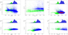 |
Fig. 3 Results of EWHα for the low-resolution data and the results of the S-index (SHK) shown in the three upper panels. The left panel shows all the data, while the middle panel provides a magnified view of the results. The right panel shows SHK. The three lower panels display the results of EWCaH, EWCaK for the low-resolution data, and EWHα for the medium-resolution data. In each panel, blue dots represent main sequence stars, while green dots represent giants. The red dots in the SHK result panel are sourced from Zhang et al. (2020). |
3.1.3 Activity-rotation relations and Ro based on Hα
The rotation of stars is intricately linked with their activity. For instance, rotation can impact the Coriolis force, thereby influencing fluid dynamics processes. Stars exhibiting faster rotation experience stronger Coriolis forces, which can intensify meridional circulation and enhance their magnetic activity. Thus, we delve into the relationship between stellar rotation periods and chromospheric activity. To compile comprehensive data, we reference various prior studies (Watson et al. 2006; McQuillan et al. 2014; Fetherolf et al. 2023) to gather as much rotational data as possible. Subsequently, we meticulously scrutinize the VSX catalog (Watson et al. 2006) to filter out binary stars from our sample, resulting in a low-resolution dataset comprising rotation periods for 16 000 stars and a medium-resolution dataset containing rotation periods for 170 stars.
Some dynamo theories posit that the magnetic activity of late-type stars arises from the α-Ω dynamo model, which amalgamates the effects of differential rotation along latitudinal directions and helical turbulence in radial directions. To explore the influence of motions in both dimensions on chromospheric activity, we compute Ro, defined as the ratio of the rotation period to the convective turnover timescale (Ro=Prot/τ), Wright et al. (2011) utilized an empirical formula correlated with stellar mass to estimate τ. Subsequently, this empirical formula has undergone updates in subsequent studies (Wright et al. 2018). To make a direct comparison with previous work, we have still adopted the empirical formula provided in Wright et al. (2011) for this study. The specific formula is as follows:
 (6)
(6)
We computed τ using the latest empirical formulas and subsequently employed Ro=Prot/τ derive Ro. Upon obtaining the periods and Ro values, we depicted their relationship with R′Hα in the following figures. The top-left panel of Figure 5 illustrates the correlation between Prot and R′Hα. Notably, when Prot is less than one day, R′Hα remains independent of Prot . However, as Prot exceeds one day, R′Hα decreases with an increase in Prot . In the top-left panel of Figure 6, we depict the relationship between Ro and R′Hα . Generally, this relationship is bifurcated into two regions: a saturated region and a non-saturated region (Douglas et al. 2014; Newton et al. 2017; Fang et al. 2018). In the saturated region, Ro exhibits independence from R′Hα. Conversely, in the non-saturated region, R′Hα decreases with an increase in Ro. Consequently, we fitted our results into two distinct parts employing the following formula as a reference:
 (7)
(7)
where Rosat represents the threshold value distinguishing the saturated region from the non-saturated region, and (R′Hα)sat denotes the corresponding R′Hα for the saturated region. Ultimately, we obtained the optimal fitting result at Rosat = 0.09 ± 0.01, with β = −0.32 ± 0.01 and (R′Hα)sat = 10−4.00±0.01. The fitting outcomes are depicted by a red dashed line in the left panel of Figure 6. Meanwhile, the blue dashed line in the panel represents the findings of Douglas et al. (2014), whose results indicate that when  . comparing our results to theirs, our Rosat and β values are within three times their standard deviation.
Due to the limited number of final parameter results available in the medium-resolution data set, which amounts to only 170 stars-most of which are relatively low-activity F and G-type stars with larger Ro statistical results cannot be well established. Therefore, in the results presented in Figures 5 and 6, we only plot the results from the low-resolution data set. All low-resolution data results related to the Hα line are shown in Table A.1 and the medium-resolution data results are shown in Table A.2.
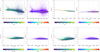 |
Fig. 4 Baseline fits for EWHα (from both medium and low-resolution data), shown in the upper two panels, and the lower two panels show E WCaK and EWCaH (both from low-resolution data), along with the results after subtracting the baseline. The solid red line in the figure depicts the fitting line for the least active 2% of stars in the sample, while the black dashed line represents y=0. In the panel without subtracting the baseline, the color bar indicates the parameter log 𝑔. In the panel after subtracting the baseline, the color bar represents the number density. |
3.2 Ca II H&K
3.2.1 S-index
In addition to Hα line, Ca II H&K lines are also widely recognized as indicators of stellar chromospheric activity (Karoff et al. 2016). Previous studies investigating the Ca II H&K lines typically employed the S-index as a quantifier of stellar chromospheric activity (Isaacson & Fischer 2010; Zhao et al. 2013). Vaughan et al. (1978) defined the S-index as the ratio of the flux of the Ca II H&K lines to that of the surrounding continuum. The calculation formula is as follows:
 (8)
(8)
where K and H respectively represent the flux within a triangular area with a full-width-at-half maximum of 1.09 Å centered at 3933.7 Å and 3968.5 Å. This is what was obtained after we resampled this portion of the spectral data. Then, V and R denote the flux within rectangular areas centered at 3901 Å and 4001 Å with a width of 20 Å. α is a constant determined by the normalization factor and the ratio of the width of the continuum window to the spectral line window. Zhang et al. (2020) utilized LAMOST low-resolution spectra to compute the S-index for FGK type main sequence stars in the Kepler field. For consistency, we adopted the same α value as theirs for calculating the S-index. In the upper right panel of Figure 3. we depict the S-index of our sample compared with that of Zhang et al. (2020). Here, blue and green dots represent the results of main sequence stars and giants in our sample, respectively. Notably, the S-index of main-sequence stars in our sample exhibits a high level of consistency with the findings of Zhang et al. (2020). Specifically, the S-index of main sequence stars increases with decreasing (Teff), aligning with previous studies indicating stronger chromospheric activity in cooler dwarfs. Similar to the Hα line, we observe that the S-index level of the giant sample is lower than that of main- equence stars, particularly in the low-temperature region. This finding corroborates the results of Zhao et al. (2013) and Zhang et al. (2023) where both studies combined main-sequence stars and giant stars for statistical analysis and demonstrated a similar distribution of S-index to our results. In particular, they are divided into two segments in the low-temperature region.
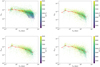 |
Fig. 5 Relationship between R′Hα , R′HK , R′CαK , and R′CaH in relation to Prot. The red dots within the figure represent the median value of each bin. |
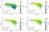 |
Fig. 6 Relationships between R′Hα, R′HK, R′CaK, and R′CaH with Ro. The red solid line represents the fit to the data, and the red shaded area indicates the error range of the fit. |
3.2.2 R′HK, R′CaH, and R′CaK
The S-index, determined by both spectral line flux and continuous spectrum flux at both ends, is sensitive to both spectral type or (Teff). Middelkoop (1982) introduced a correlation factor, Ccf , based on the B-V color to convert the S-index into the surface flux of FH + FK. Noyes et al. (1984) introduced R′HK as a more accurate measure of chromospheric emission, calculated as RHK – Rphot. Schrijver (1987) further refined this by subtracting the basal chromospheric flux using the B-V color. Isaacson & Fischer (2010) and Zhao et al. (2015) utilized both the S-index and the basal S-index (the fitted value for the least active 5% of their sample) to mitigate the influence of (Teff ) and spectral type on the S-index. In our study, we adopted a method consistent with theirs to eliminate the (Teff) and spectral type on SHK. This method is aligned with the approach we previously utilized for R′Hα. Subsequently, we computed the ratio of the Ca II H&K lines to the bolometric luminosity, denoted as R′HK.
To facilitate comparison with the quantification results of Hα lines, in addition to computing the R′HK, we also computed the EW′CaH, EW′Cak, R′H, and R′K of the Ca II H&K lines. The cal-cuation process closely mirrors that of the Hα line, with the only variations given in the central wavelength position and the continuum spectral range. Fang et al. (2018) previously calculated the EW of the Ca II K line, selecting a spectral range of 3930– 3937 Å and continuum spectral ranges of 3910–3915 Å and 3950–3955 Å. In alignment with the slightly wider range chosen for the Hα line, we opted for a spectral range of 3929–3938 Å, maintaining consistency in the continuum spectral range.
Similarly, for the Ca II H line, our chosen spectral range is 3964–3973 Å, with continuum coverage in the ranges of 3950–3955 Å and 3995–4000 Å. The specific calculation process is shown in the following formula:
 (9)
(9)
 (10)
(10)
 (11)
(11)
 (12)
(12)
 (13)
(13)
 (14)
(14)
 (15)
(15)
where FH and FK are calculated in a similar manner to FHα, both derived using the PHOENIX ACES. Also, EWCaH,basal and E WCaK,basal denotes the basal chromospheric flux, derived by fitting the least active stars in our sample.
The results of EW Ca II K and EW Ca II H are presented in the bottom-left panel and bottom-middle panel in Figure 3. Blue and green dots representing main sequence stars and giant stars, respectively. Following the processing method applied to the Hα line, we computed EW′CaK and EW′CaH, shown in the four panels below Figure 4. Furthermore, we examined the correlation between R′Hα, R′HK, R′CaH, and R′CaK in Figure 7. The black dashed line in the figure represents the straight line fit of the results, revealing a clear linear relationship where both R′CaH and R′CaK increase with the rise in Hα.
3.2.3 Activity–rotation relations and Ro based on Ca II H&K
Utilizing the method outlined in Section 3.1.3, we derived the Prot and Ro for approximately 8000 stars. These results were distinguished and plotted in Figures 5 and 6. In Figure 5, the upper right panel and the lower two panels depict the relationships between stellar magnetic activity parameters R′HK, R′CaH, R′CaK, and Prot, respectively. The red dots represent the median in each bin. It’s evident that when Prots less than 1 day, R′HK, R′CaH and R′CaK exhibit minimal variation with Prot. However, when Prot exceeds 1 day, these parameters gradually decrease with Prot increase.
Similarly, the upper right panel and the lower two panels in Figure 6 illustrate the relationships between these parameters and Ro. Employing the same fitting method as in the relationship between Hα and Ro, we obtain Rosat = 0.11 ± 0.01, β = −0.49 ± 0.01, and (R′HK)sat = 10−3.97±0.02. For R′CaH, we obtained Rosat = 0.12 ± 0.01, β = −0.56 ± 0.02 and (R′CaH)sat = 10−4.00±0.02. And for R′CaK, we obtain Rosat = 0.11 ± 0.01, β = −0.47 ± 0.01 and (R′CaK)sat = 10−3.95±0.02. Notably, the β values in these results are higher than the 0.32 found for the Hα line, consistent with the findings of Pasquini & Pallavicini (1991), indicating that the variation of the Hα flux with stellar activity is slightly slower than that of Ca II H&K. Furthermore, the critical values of these two regions typically range between 0.1 and 0.3. For instance, Douglas et al. (2014) and Newton et al. (2017) found critical values around  and 0.21 ±0.02, respectively, using the Hα line. Fang et al. (2018) suggested a critical value above 0.2, even reaching 0.27, based on Hα, Hβ, and Ca II K spectral lines.
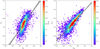 |
Fig. 7 Relationship between R′Hα and R′HK (left). Relationship between R′CaH and R′CaK (right). The black dashed line in the two panels represents the result fitted using the Monte Carlo method and the shaded area indicates the fitting error. |
3.3 EW variability of chromospheric activity indicators
Finally, we calculated the variation of the EWs of Hα, Ca II H, and Ca II K lines for stars with multiple observations in the low- resolution dataset, as well as the variation of the EW of Hα for all samples in the medium-resolution dataset. We calculated the changes in various chromosphere activity indicators using the following formula (Long et al. 2021; Zhang et al. 2023):
 (16)
(16)
Here i represents Hα, Ca II H, and Ca II K. In the low- resolution dataset, we have identified more than 2900 stars exhibiting obvious EW variations in the Hα line, 5700 stars in Ca II line, and 8400 stars in Ca II K. This indicates that compared to Hα line, Ca II H&K lines are more sensitive indicator of variation of chromospheric activity. In the medium-resolution dataset, 719 stars have been identified as exhibiting significant EW variations in the Hα line. Usually, stars with drastic variation in chromospheric activity indicators have stronger activity. These stars with exhibiting obvious chromospheric activity variations are not ideal samples for the search for exoplanets. All low-resolution data results related to the Ca II K lines are shown in Table A.1.
3.4 The priority of ET 2.0 observations
Utilizing LAMOST low-resolution spectra, We have established the observation priorities for the ET 2.0 field of view. The priority decreases sequentially from 0 to 4. To ensure that the stars we exclude are all those with strong activity, we selected an EW′Hα value greater than 0.2 as the threshold. 0.2 is three times the median of the EW′Hα,err . Compared to 0, this allows us to include more observational samples while avoiding misclassification of non-active stars due to S/N effects. Priority 0 means EW′CaK , EW′CaH, and EW′Hα are all less than 0.2, and none of the three spectral lines exhibit variability. Priority 1 contains two types of samples. The first type is when the EW′Hα line is less than 0.2 and the spectral lines do not exhibit variability. The second type is when the EW′CaK and EW′CaH lines are both less than 0.2 and the spectral lines do not exhibit variability. Priority 2 indicates that EW′CaK , EW′CaH and EW′Hα are all less than 0.2, but the spectral lines have variability (or only one observation) making it impossible to determine whether the spectral lines have variability. Priority 3 indicates that EW′CaK and EW′CaH are less than 0.2, or EW′Hα is less than 0.2, but the spectral lines exhibit variability (or there is only one observation), making it impossible to determine variability. Priority 4 indicates that EW′CaK , EW′CaH and EW′Hα are all greater than 0.2, belonging to samples with relatively strong activity. The activity level for those not specified falls between priorities 3 and 4. The priorities are displayed in the last column of Table A.1.
4 Summary
This study delves into the chromospheric activity of stellar sources observed by LAMOST within the ET 2.0 field. The key findings are summarized below:
Chromospheric activity analysis: we conducted chromospheric activity characterization for over 320 000 spectra using Hα lines and over 110 000 spectra using Ca II H&K lines.
Selection of observational targets: utilizing LAMOST low- and medium-resolution spectra, we determined the priority of the observational target for ET 2.0.
Correlation between active indicators: positive relationships were observed among different active indicators: R′Hα–R′HK and R′CaK –R′CaH.
Revised activity–rotation relations: we revisited the relationship between stellar activity and rotation, confirming the presence of two distinct regions: saturated and unsaturated. Our results have yielded a critical value between 0.09 and 0.12, in agreement with previous findings (Douglas et al. 2014). Additionally, we observed that Ca II H&K lines exhibit greater sensitivity to Ro than Hα line in the unsaturated region.
In summary, this work determined the chromospheric activity intensity of stars in the ET field based on LAMOST observation targets, expanded the sample of chromospherically active stars, and provided valuable references for the future observation targets of the ET 2.0 project.
Data availability
The Full Tables A.1 and A.2 are available at the CDS via anonymous ftp to cdsarc.cds.unistra.fr (130.79.128.5) or via https://cdsarc.cds.unistra.fr/viz-bin/cat/J/A+A/694/A157
Acknowledgements
Our research is supported by the NSFC awards No. 12373032 and 11963002. This paper is based on the data of LAMOST, a National Major Scientific Project built by the Chinese Academy of Sciences. We also thank the supports by the science research grants from the China Manned Space Project with No. CMS-CSST-2021-B07. Thank you to the Talent Program of the Guizhou Science and Technology Cooperation Platform – ZDSYS[2023]003 for the support.
Appendix A Table
Low-resolution spectral parameters.
Medium-resolution spectral parameters
References
- Antiochos, S. K., DeVore, C. R., & Klimchuk, J. A. 1999, ApJ, 510, 485 [Google Scholar]
- Babcock, H. W. 1958, ApJS, 3, 141 [Google Scholar]
- Ballerini, P., Micela, G., Lanza, A. F., et al. 2012, A&A, 539, A140 [NASA ADS] [CrossRef] [EDP Sciences] [Google Scholar]
- Berdyugina, S. V. 2005, Liv. Rev. Sol. Phys., 2, 8 [Google Scholar]
- Browning, M. K., Basri, G., Marcy, G. W., et al. 2010, AJ, 139, 504 [NASA ADS] [CrossRef] [Google Scholar]
- Casagrande, L., Flynn, C., & Bessell, M. 2008, MNRAS, 389, 585 [Google Scholar]
- Ciardi, D. R., von Braun, K., Bryden, G., et al. 2011, AJ, 141, 108 [Google Scholar]
- Cui, X.-Q., Zhao, Y.-H., Chu, Y.-Q., et al. 2012, Res. Astron. Astrophys., 12, 1197 [Google Scholar]
- Delfosse, X., Forveille, T., Perrier, C., et al. 1998, A&A, 331, 581 [NASA ADS] [Google Scholar]
- Douglas, S. T., Agüeros, M. A., Covey, K. R., et al. 2014, ApJ, 795, 161 [NASA ADS] [CrossRef] [Google Scholar]
- Fang, X.-S., Zhao, G., Zhao, J.-K., et al. 2016, MNRAS, 463, 2494 [NASA ADS] [CrossRef] [Google Scholar]
- Fang, X.-S., Zhao, G., Zhao, J.-K., et al. 2018, MNRAS, 476, 908 [NASA ADS] [CrossRef] [Google Scholar]
- Fetherolf, T., Pepper, J., Simpson, E., et al. 2023, ApJS, 268, 4 [NASA ADS] [CrossRef] [Google Scholar]
- Frasca, A., Molenda-Zakowicz, J., De Cat, P., et al. 2016, A&A, 594, A39 [CrossRef] [EDP Sciences] [Google Scholar]
- Gaia Collaboration (Brown, A. G. A., et al.) 2021, A&A, 649, A1 [NASA ADS] [CrossRef] [EDP Sciences] [Google Scholar]
- Gaia Collaboration (Vallenari, A., et al.) 2023, A&A, 674, A1 [NASA ADS] [CrossRef] [EDP Sciences] [Google Scholar]
- Ge, J., Zhang, H., Zang, W., et al. 2022, arXiv e-prints [arXiv:2206.06693] [Google Scholar]
- Gunn, A. G., & Doyle, J. G. 1997, A&A, 318, 60 [NASA ADS] [Google Scholar]
- Hawley, S. L., Gizis, J. E., & Reid, I. N. 1996, AJ, 112, 2799 [Google Scholar]
- Hawley, S. L., Covey, K. R., Knapp, G. R., et al. 2002, AJ, 123, 3409 [NASA ADS] [CrossRef] [Google Scholar]
- Hawley, S. L., Davenport, J. R. A., Kowalski, A. F., et al. 2014, ApJ, 797, 121 [Google Scholar]
- He, H., Zhang, W., Zhang, H., et al. 2023, Ap&SS, 368, 63 [CrossRef] [Google Scholar]
- Herbig, G. H. 1985, ApJ, 289, 269 [NASA ADS] [CrossRef] [Google Scholar]
- Husser, T.-O., Wende-von Berg, S., Dreizler, S., et al. 2013, A&A, 553, A6 [NASA ADS] [CrossRef] [EDP Sciences] [Google Scholar]
- Isaacson, H., & Fischer, D. 2010, ApJ, 725, 875 [Google Scholar]
- Karoff, C., Knudsen, M. F., De Cat, P., et al. 2016, Nat. Commun., 7, 11058 [NASA ADS] [CrossRef] [Google Scholar]
- Kay, C., Opher, M., & Kornbleuth, M. 2016, ApJ, 826, 195 [NASA ADS] [CrossRef] [Google Scholar]
- Koch, D. G., Borucki, W. J., Basri, G., et al. 2010, ApJ, 713, L79 [Google Scholar]
- Kraft, R. P. 1967, ApJ, 150, 551 [Google Scholar]
- Leighton, R. B. 1969, ApJ, 156, 1 [Google Scholar]
- Lingam, M., & Loeb, A. 2017, ApJ, 848, 41 [Google Scholar]
- Linsky, J. L., Redfield, S., & Tilipman, D. 2019, ApJ, 886, 41 [NASA ADS] [CrossRef] [Google Scholar]
- Liu, C., Fu, J., Shi, J., et al. 2020, arXiv e-prints [arXiv:2005.07210] [Google Scholar]
- Long, L., Zhang, L.-y., Bi, S.-L., et al. 2021, ApJS, 253, 51 [NASA ADS] [CrossRef] [Google Scholar]
- Lu, H.-p., Zhang, L.-y., Shi, J., et al. 2019, ApJS, 243, 28 [NASA ADS] [CrossRef] [Google Scholar]
- Lu, H.-p., Tian, H., Zhang, L.-y., et al. 2022, A&A, 663, A140 [NASA ADS] [CrossRef] [EDP Sciences] [Google Scholar]
- Luo, A.-L., Zhao, Y.-H., Zhao, G., et al. 2015, Res. Astron. Astrophys., 15, 1095 [Google Scholar]
- Mamajek, E. E., & Hillenbrand, L. A. 2008, ApJ, 687, 1264 [Google Scholar]
- Mayor, M., & Queloz, D. 1995, Nature, 378, 355 [Google Scholar]
- Mayor, M., Pepe, F., Queloz, D., et al. 2003, The Messenger, 114, 20 [NASA ADS] [Google Scholar]
- McQuillan, A., Mazeh, T., & Aigrain, S. 2014, ApJS, 211, 24 [Google Scholar]
- Middelkoop, F. 1982, A&A, 107, 31 [NASA ADS] [Google Scholar]
- Mihalas, D. 1978, Stellar atmospheres (San Francisco: W.H. Freeman) [Google Scholar]
- Mittag, M., Schmitt, J. H. M. M., & Schröder, K.-P. 2013, A&A, 549, A117 [NASA ADS] [CrossRef] [EDP Sciences] [Google Scholar]
- Mohanty, S., & Basri, G. 2003, ApJ, 583, 451 [NASA ADS] [CrossRef] [Google Scholar]
- Montes, D., Fernandez-Figueroa, M. J., de Castro, E., et al. 1995, A&A, 294, 165 [NASA ADS] [Google Scholar]
- Montes, D., Martin, E. L., Fernandez-Figueroa, M. J., et al. 1997, A&AS, 123, 473 [NASA ADS] [CrossRef] [EDP Sciences] [Google Scholar]
- Newton, E. R., Irwin, J., Charbonneau, D., et al. 2017, ApJ, 834, 85 [Google Scholar]
- Noyes, R. W., Hartmann, L. W., Baliunas, S. L., et al. 1984, ApJ, 279, 763 [NASA ADS] [CrossRef] [Google Scholar]
- Parker, E. N. 1955, ApJ, 121, 491 [Google Scholar]
- Pasquini, L., & Pallavicini, R. 1991, A&A, 251, 199 [NASA ADS] [Google Scholar]
- Reiners, A., Basri, G., & Browning, M. 2009, ApJ, 692, 538 [NASA ADS] [CrossRef] [Google Scholar]
- Reiners, A., Joshi, N., & Goldman, B. 2012, AJ, 143, 93 [Google Scholar]
- Reinhold, T., & Hekker, S. 2020, A&A, 635, A43 [NASA ADS] [CrossRef] [EDP Sciences] [Google Scholar]
- Ricker, G. R., Winn, J. N., Vanderspek, R., et al. 2014, Proc. SPIE, 9143, 914320 [Google Scholar]
- Robertson, P., Roy, A., & Mahadevan, S. 2015, ApJ, 805, L22 [NASA ADS] [CrossRef] [Google Scholar]
- Schrijver, C. J. 1987, A&A, 172, 111 [NASA ADS] [Google Scholar]
- Schrijver, C. J., Cote, J., Zwaan, C., et al. 1989, ApJ, 337, 964 [NASA ADS] [CrossRef] [Google Scholar]
- Stauffer, J. R., & Hartmann, L. W. 1986, ApJS, 61, 531 [NASA ADS] [CrossRef] [Google Scholar]
- Stauffer, J. R., & Hartmann, L. W. 1987, ApJ, 318, 337 [NASA ADS] [CrossRef] [Google Scholar]
- Strassmeier, K. G. 2009, A&A Rev., 17, 251 [NASA ADS] [CrossRef] [Google Scholar]
- Su, T., Zhang, L.-y., Long, L., et al. 2022, ApJS, 261, 26 [NASA ADS] [CrossRef] [Google Scholar]
- Thomas, B. C., Jackman, C. H., & Melott, A. L. 2007, Geophys. Res. Lett., 34, L06810 [NASA ADS] [Google Scholar]
- Tu, Z.-L., Yang, M., Zhang, Z. J., et al. 2020, ApJ, 890, 46 [NASA ADS] [CrossRef] [Google Scholar]
- Tu, Z.-L., Yang, M., Wang, H.-F., et al. 2021, ApJS, 253, 35 [NASA ADS] [CrossRef] [Google Scholar]
- Vaughan, A. H., & Preston, G. W. 1980, PASP, 92, 385 [Google Scholar]
- Vaughan, A. H., Preston, G. W., & Wilson, O. C. 1978, PASP, 90, 267 [Google Scholar]
- Walkowicz, L. M., Hawley, S. L., & West, A. A. 2004, PASP, 116, 1105 [CrossRef] [Google Scholar]
- Wang, S.-G., Su, D.-Q., Chu, Y.-Q., et al. 1996, Appl. Opt., 35, 5155 [NASA ADS] [CrossRef] [Google Scholar]
- Watson, C. L., Henden, A. A., & Price, A. 2006, Soc. Astron. Sci. Annu. Symp., 25, 47 [Google Scholar]
- West, A. A., Hawley, S. L., Walkowicz, L. M., et al. 2004, AJ, 128, 426 [NASA ADS] [CrossRef] [Google Scholar]
- West, A. A., Hawley, S. L., Bochanski, J. J., et al. 2008, AJ, 135, 785 [Google Scholar]
- Wilson, O. C. 1963, ApJ, 138, 832 [NASA ADS] [CrossRef] [Google Scholar]
- Wilson, O. C. 1968, ApJ, 153, 221 [Google Scholar]
- Wilson, O. C., & Skumanich, A. 1964, ApJ, 140, 1401 [NASA ADS] [CrossRef] [Google Scholar]
- Wolszczan, A., & Frail, D. A. 1992, Nature, 355, 145 [CrossRef] [Google Scholar]
- Wright, N. J., Drake, J. J., Mamajek, E. E., et al. 2011, ApJ, 743, 48 [NASA ADS] [CrossRef] [Google Scholar]
- Wright, N. J., Newton, E. R., Williams, P. K. G., et al. 2018, MNRAS, 479, 2351 [NASA ADS] [CrossRef] [Google Scholar]
- York, D. G., Adelman, J., Anderson, J. E., et al. 2000, AJ, 120, 1579 [Google Scholar]
- Zhang, L., Pi, Q., Han, X. L., et al. 2016, New A, 44, 66 [Google Scholar]
- Zhang, L., Lu, H., Han, X. L., et al. 2018, New A, 61, 36 [NASA ADS] [CrossRef] [Google Scholar]
- Zhang, J., Bi, S., Li, Y., et al. 2020, ApJS, 247, 9 [NASA ADS] [CrossRef] [Google Scholar]
- Zhang, L.-y., Meng, G., Long, L., et al. 2021, ApJS, 253, 19 [NASA ADS] [CrossRef] [Google Scholar]
- Zhang, L.-. Y., Su, T., Misra, P., et al. 2023, ApJS, 264, 17 [NASA ADS] [CrossRef] [Google Scholar]
- Zhang, J., Xiang, M., Yu, J., et al. 2024, ApJS, 272, 40 [CrossRef] [Google Scholar]
- Zhao, G., Zhao, Y.-H., Chu, Y.-Q., et al. 2012, Res. Astron. Astrophys., 12, 723 [CrossRef] [Google Scholar]
- Zhao, J. K., Oswalt, T. D., Zhao, G., et al. 2013, AJ, 145, 140 [Google Scholar]
- Zhao, J.-K., Oswalt, T. D., Chen, Y.-Q., et al. 2015, Res. Astron. Astrophys., 15, 1282 [CrossRef] [Google Scholar]
All Tables
All Figures
|
Fig. 1 LAMOST DR10 low-resolution and medium-resolution samples in the ET 2.0 field, presented in the three panels above and the three panels below, respectively. The left, middle, and right panels of each set of images represent the relationship diagrams of different physical parameters. Left panel: HRD based on Gaia DR3 data. The color bar indicates the number density of stars. Middle panel: The relationship diagram between (Teff) and log 𝑔 based on LAMOST DR10 data, with the color bar representing the parameter [Fe/H]. The black dashed line represents the empirical formula proposed by Ciardi et al. (2011). Dividing the samples into giant stars (above the line) and main-sequence stars (below the line). Right panel: relationship diagram between (Teff) and log g based on LAMOST DR10 data, with the color bar indicating the number density of stars. |
| In the text | |
|
Fig. 2 S/N distribution statistics for the u and r bands of the low-resolution data (left panels). S/N distribution statistics for the r band of the medium-resolution data (right panels). |
| In the text | |
|
Fig. 3 Results of EWHα for the low-resolution data and the results of the S-index (SHK) shown in the three upper panels. The left panel shows all the data, while the middle panel provides a magnified view of the results. The right panel shows SHK. The three lower panels display the results of EWCaH, EWCaK for the low-resolution data, and EWHα for the medium-resolution data. In each panel, blue dots represent main sequence stars, while green dots represent giants. The red dots in the SHK result panel are sourced from Zhang et al. (2020). |
| In the text | |
|
Fig. 4 Baseline fits for EWHα (from both medium and low-resolution data), shown in the upper two panels, and the lower two panels show E WCaK and EWCaH (both from low-resolution data), along with the results after subtracting the baseline. The solid red line in the figure depicts the fitting line for the least active 2% of stars in the sample, while the black dashed line represents y=0. In the panel without subtracting the baseline, the color bar indicates the parameter log 𝑔. In the panel after subtracting the baseline, the color bar represents the number density. |
| In the text | |
|
Fig. 5 Relationship between R′Hα , R′HK , R′CαK , and R′CaH in relation to Prot. The red dots within the figure represent the median value of each bin. |
| In the text | |
|
Fig. 6 Relationships between R′Hα, R′HK, R′CaK, and R′CaH with Ro. The red solid line represents the fit to the data, and the red shaded area indicates the error range of the fit. |
| In the text | |
|
Fig. 7 Relationship between R′Hα and R′HK (left). Relationship between R′CaH and R′CaK (right). The black dashed line in the two panels represents the result fitted using the Monte Carlo method and the shaded area indicates the fitting error. |
| In the text | |
Current usage metrics show cumulative count of Article Views (full-text article views including HTML views, PDF and ePub downloads, according to the available data) and Abstracts Views on Vision4Press platform.
Data correspond to usage on the plateform after 2015. The current usage metrics is available 48-96 hours after online publication and is updated daily on week days.
Initial download of the metrics may take a while.