| Issue |
A&A
Volume 694, February 2025
|
|
|---|---|---|
| Article Number | A140 | |
| Number of page(s) | 17 | |
| Section | Extragalactic astronomy | |
| DOI | https://doi.org/10.1051/0004-6361/202451805 | |
| Published online | 10 February 2025 | |
Spectral energy distribution modelling of broad emission line quasars: From X-ray to radio wavelengths
1
INAF – Osservatorio Astrofisico di Arcetri, Largo E. Fermi 5, 50125 Firenze, Italy
2
School of Astrophysics, Presidency University Kolkata 700073, India
3
International Gemini Observatory/NSF NOIRLab, Casilla 603, La Serena, Chile
4
Laboratório Nacional de Astrofísica, MCTI, Rua dos Estados Unidos, 154, Bairro das Nações, Itajubá, MG 37501-591, Brazil
5
Department of Physics, Presidency University, Kolkata 700073, India
⋆ Corresponding author; This email address is being protected from spambots. You need JavaScript enabled to view it.
Received:
5
August
2024
Accepted:
21
November
2024
Abstract
Aims. We study differences in the physical properties of quasar host galaxies using an optically selected sample of radio-loud (RL) and radio-quiet quasars (in the redshift range 0.15 ≤ z ≤ 1.9) that we have further cross-matched with the VLA-FIRST survey catalogue. The sources in our sample have broad Hβ and Mg II emission lines (1000 km/s < FWHM < 15 000 km/s) with a sub-sample of high broad-line quasars (FWHM > 15 000 km/s). We constructed the broad-band spectral energy distribution (SED) of our broad-line quasars using multi-wavelength archival data and targeted observations with the AstroSat telescope.
Methods. We used the state-of-the-art SED modelling code CIGALE v2022.0 to model the SEDs and determine the best-fit physical parameters of the quasar host galaxies; namely, their star formation rate (SFR), main-sequence stellar mass, luminosity absorbed by dust, e-folding time, and stellar population age.
Results. We find that the emission from the host galaxy of our sources is between 20% and 35% of the total luminosity, as they are mostly dominated by central quasars. Using the best-fit estimates, we reconstructed the optical spectra of our quasars, which show remarkable agreement in reproducing the observed SDSS spectra of the same sources. We plot the main-sequence relation for our quasars and note that they are significantly away from the main sequence of star-forming galaxies. Further, the main-sequence relation shows a bimodality for our RL quasars, indicating populations segregated by Eddington ratios.
Conclusions. We conclude that RL quasars in our sample with lower Eddington ratios tend to have substantially lower SFRs for similar stellar mass. Our analyses thus provide a completely independent route to studying the host galaxies of quasars and addressing the radio dichotomy problem from the host galaxy angle.
Key words: catalogs / galaxies: active / quasars: emission lines
Gemini Science Fellow.
CNPq Fellow.
© The Authors 2025
 Open Access article, published by EDP Sciences, under the terms of the Creative Commons Attribution License (https://creativecommons.org/licenses/by/4.0), which permits unrestricted use, distribution, and reproduction in any medium, provided the original work is properly cited.
This article is published in open access under the Subscribe to Open model. This email address is being protected from spambots. You need JavaScript enabled to view it. to support open access publication.
1. Introduction
Quasars are the most luminous and the most distant members of the active galactic nuclei (AGN) population. Although quasars were first discovered through their strong radio jet emission (Schmidt 1963), roughly 10% of quasars are considered powerful radio sources termed radio-loud (RL) quasars (Sandage 1965); stritt; (Schmidt & Green 1983; Kellermann et al. 1989; Miller et al. 1993; Ivezić et al. 2002; Jiang et al. 2007; Rafter et al. 2011). The physical reason behind the existence of this radio dichotomy remains an unsolved problem in quasar physics (Strittmatter et al. 1980; Kellermann et al. 1989; Miller et al. 1990; Ivezić et al. 2002; White et al. 2007; Zamfir et al. 2008).
Various factors have been proposed to explain the RL–radio-quiet (RQ) divide, such as the mass and spin of the central black hole (BH) (McLure & Jarvis 2004), the different physical origin of radio emission (Laor & Behar 2008), accretion rates (Sikora et al. 2007; Hamilton 2010; Marziani et al. 2021), and the overall spectral energy distribution (SED) (Laor et al. 1997; Marziani et al. 2023). However, none of the above studies have been conclusive. One approach to addressing this radio dichotomy involves studying their host galaxy properties (Sikora et al. 2007; Lagos et al. 2009; Kimball et al. 2011). The hosts of quasars are often star-forming galaxies (see review by Heckman & Best 2014). Synchrotron radiation from electrons accelerated to relativistic speeds in supernova remnants as well as free-free emission from HII regions are produced in star formation regions (Condon 1992). It has been found that radio continuum emission at low frequencies in low-luminosity quasars is consistent with being dominated by star formation (Gürkan et al. 2019). Further, in contrast with previous studies at lower redshifts, (e.g. McLure & Dunlop 2001), Falcke et al. (1996), and Kauffmann et al. (2008) showed that RL AGNs appear to be found in denser environments than their RQ counterparts. This is in qualitative agreement with other works on higher-redshift quasars (Kalfountzou et al. 2012).
It was realised from early studies that the cosmic star formation history (SFH) (e.g. Madau et al. 1996; Hopkins & Beacom 2006) and the evolving luminosity density of quasars (e.g. Boyle & Terlevich 1998; Richards & Kratzer 2014; Croom et al. 2009) follow a similar trend (e.g. Franceschini et al. 1999). There is supporting evidence for the presence of cold gas (e.g. Evans et al. 2001; Scoville et al. 2003; Walter et al. 2004; Emonts et al. 2011), dust (Archibald et al. 2001; Page et al. 2001; Reuland et al. 2004; Stevens et al. 2005), and young stars (e.g. Tadhunter et al. 2005; Baldi & Capetti 2008; Herbert et al. 2010) in powerful RL quasars, in contrast to the composition of the normal ellipticals that usually host RL quasars (e.g. Dunlop et al. 2003).
Many studies have also attempted multi-band optical photometry (e.g. Sánchez et al. 2004) or spectroscopy (e.g. Trichas et al. 2010, 2012; Kalfountzou et al. 2011 to determine the star formation activity in quasar host galaxies. At lower redshift, the spectrophotometric data from SDSS for well-defined samples of radio galaxies have also been used to investigate differences in star formation activity and environments of quasar host galaxies (e.g. Kauffmann et al. 2003, 2004; Best et al. 2005; Best & Heckman 2012). It was found that the environment plays a relatively minor role if the radio loudness is due to the physics of the central engine and how it is fuelled. However, the quasar properties may be connected with the star formation in their host galaxies (e.g. Herbert et al. 2010; Croft et al. 2006; Silk & Nusser 2010).
The complex physical interplay between the main baryonic components of galaxies like stars, their remnants, molecular, atomic, and ionised gas, dust, and supermassive BHs causes multi-wavelength emission ranging from γ–rays to the radio domain (see e.g. Harrison 2014; Netzer 2015). The typical SED of a galaxy that covers a broad wavelength range, from X-ray to infrared (IR), therefore contains the imprint of the baryonic processes that drove its formation and evolution across cosmic time. In other words, it is important to extract the information tightly woven into the SED of galaxies across a broad range of wavelengths to understand galaxy formation and evolution. Modelling the SED of galaxies is a heavily intricate problem as it involves AGN contributions as well. Galaxies with very different properties can have broadly similar SEDs and misinterpretation of the SED could lead to unrealistic physical conclusions. This is particularly the case when we do not consider the full SED.
In our previous studies, using the Sloan Digital Sky Survey Data Release 7 quasar catalogue we selected a sample of RL and RQ quasars through their broad Hβ and Mg II full width at half maximum (FWHM) (Chakraborty & Bhattacharjee 2021; Chakraborty et al. 2021, 2022). Our results revealed that the RL fraction (RLF) increases with FWHM for both broad Hβ and Mg II samples. To understand this effect, we further selected a sub-sample with FWHMs greater than 15 000 km s−1 (HBL hereafter) from both Hβ and Mg II samples and performed a systematic study of the different AGN properties; namely, the bolometric luminosity, BH mass, optical continuum luminosity, and Eddington ratio. To search for possible reasons for higher RLF, we further constructed and compared the composite SDSS spectra of the RL and RQ quasars for our Hβ sample. We also compared the BH mass, Eddington ratio, bolometric luminosity, Hβ FWHM, and RFe (i.e. the flux ratio of the optical Fe II emission within 4434–4684 Å to the broad Hβ emission) of our sample with the rest of the Hβ broad emission line objects; that is, an FWHM of less than 15 000 km s−1 (non-HBL hereafter). We found that the luminosities are different but BH mass and Eddington ratios are similar for RL and RQ HBL. The accretion disc luminosity of the RL quasars in our HBL sample is higher, which indicates a connection between a brighter disc and a more prominent jet. By comparing them with the non-HBL broad emission line quasars, we found that the HBL sources have the lowest Eddington ratios in addition to having a very high RLF. We also found that the [O III] narrow emission line is stronger in the RL compared to the RQ quasars in our HBL sample.
In addition to their intrinsic differences, we anticipate the presence of a radio jet having a distinct effect on its host galaxy. In this work, we compare the physical properties of the RL and RQ quasar-hosting galaxies of broad Hβ and Mg II samples by modelling their SEDs with the CIGALE v2022.01 code (Yang et al. 2022). This analysis allows us to examine the radio dichotomy problem from the angle of host galaxies of our RL and RQ quasars. The paper is organised as follows. In Sect. 2, we lay out the construction of our dataset and discuss our methodology for modelling the broad-band SED of our sources. In Sect. 3, we report our results. Finally, we discuss our results and summarise our main conclusions in Sect. 4.
2. Methodology
We now describe our methodology for the construction and modelling of the broad-band SEDs of our quasar sample.
2.1. Datasets
Our main quasar sample is drawn from the SDSS (York et al. 2000) Data Release 7 (Abazajian et al. 2009) quasar catalogue (Shen et al. 2011). It consists of 105 783 quasars brighter than Mi = −22.0 that have been spectroscopically confirmed and taken from ∼9380 sq. deg of the sky. The catalogue consists of quasars that have reliable redshifts and have at least one emission line (Hβ and Mg II) with an FWHM greater than 1000 km s−1. The flux limit for the main spectroscopic sample is i < 19.1; hence, the majority of quasars are brighter than i ≈ 19 within the redshift limit of z < 1.9, which include broad Hβ and Mg II line samples. We have chosen to use DR7 because it contains all the BH masses and includes line fits with multiple Gaussian functions for the broad Hβ and Mg II lines. Except for the C IV emission line, different procedures to measure the broad Hβ and Mg II have been adopted (Shen et al. 2008; McLure & Dunlop 2004), and different fiducial scaling relations to compute Hβ- and Mg II-based virial BH masses are used.
Shen et al. (2011) cross-matched the quasar catalogue of SDSS DR7 with the FIRST survey (White et al. 2007). The quasars that have only one FIRST source within 5″ are classified as core-dominated radio sources and those that have multiple FIRST sources within 30″ are classified as lobe-dominated. These two categories are together termed as RL quasars by Shen et al. (2011). Quasars with only one FIRST match between 5″ and 30″ are classified as FIRST non-detections and as RQ quasars. The SDSS sample contains 105,783 quasars, of which 99 182 have FIRST counterparts. Among these, 9399 are RL quasars and 88 979 are RQ ones.
Furthermore, these RL and RQ samples were cross-matched with WISE (Wright et al. 2010) for IR counterparts. The WISE cross-matching left the sample size for RL and RQ quasars as 959 and 7252, respectively. Next, the sample was cross-matched with GALEX (Martin et al. 2005) for UV counterparts, where 186 and 74 counterparts were found for RL and RQ quasars, respectively. Among these sources, three RL sources and two RQ ones are HBL. Lastly, for X-ray counterparts, our sample was cross-matched with Chandra (Evans et al. 2010), ROSAT (Truemper 1982), Swift (Tueller et al. 2008), and XMM-Newton (Bianchi et al. 2009). The cross-matching with the X-ray catalogues was conducted within a radius of 3 arcseconds of our sources (Svoboda et al. 2017). This sample (non-HBL hereafter) consists of 31 RL and 14 RQ quasars in the redshift range 0.33 < z < 1.88, with at least one broad emission line (Hβ or Mg II). After cross-matching with X-rays, our sample do not contain any HBL source. However, we added three RL HBL sources and two RQ ones to our sample (HBL hereafter) without the X-ray data. Including the HBL sources, our sample consists of 34 RL (Table A.1) and 16 RQ (Table B.1) quasars. We note that we also cross-matched our sources with the 2MASS catalogue (Skrutskie et al. 2006) for near-IR coverage. We found 17 matches consisting of both the RL and RQ populations. For the 17 2MASS matches, we performed the SED analysis with and without the 2MASS data point. Our results indicate that the derived host galaxy properties with and without the 2MASS data are statistically similar. Adding the 2MASS sources would have significantly reduced our sample size, and hence we did not include the 2MASS analysis in this work.
While constructing the broad-band SED, we found that some of our sources have near-UV (NUV) but no far-UV (FUV) observations in GALEX. For those sources, we performed observations of a sample of three RL quasars and three RQ ones in the FUV band using the Ultraviolet Imaging Telescope (UVIT) on board AstroSat (Proposal ID: A11_047). These six sources in particular were selected based on their low exposure time requirement for observation. After including the six AstroSat sources, our final sample consists of 37 RL sources and 19 RQ ones (0.15 < z < 1.88; Fig. 1). We briefly discuss the UVIT data reduction here.
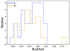 |
Fig. 1. Histograms of redshift for the non-HBL+HBL+AstroSat-observed RL (dashed blue) and RQ (solid orange) sources in our sample. Our datasets are described in Sect. 2.1. |
For the analysis of our AstroSat sources, we obtained the Level 1 (L1) UVIT data from the AstroSat data archive2, which we processed using the CCDLAB pipeline (Postma & Leahy 2017), to generate orbitwise cleaned images. CCDLAB applies various detector and satellite corrections to the L1 data, such as corrections for the flat field, centroiding bias, and pointing drift. Using CCDLAB, we aligned and merged the orbitwise images into a final image for each observation. Astrometry of the final images using CCDLAB was performed for two sources (SDSS 085605.83+450520.0 and SDSS 085605.83+450520.0).
For the other four observations, identification of the source of interest was done by comparing the UVIT field of view with the same field in NUV from the GALEX All-sky Imaging Survey using SIMBAD. We then performed aperture photometry on the final images using standard Python tools, astropy and photutils. For all the sources, we extracted the source counts from circular regions with radii of 25 pixels centred on the source. Background counts were extracted from nearby circular regions with 60-pixel radii. Finally, we converted the background-corrected source count rates to respective flux (fλ) and magnitude values using the UVIT zero point flux and magnitude information provided by Tandon et al. (2020). The observed flux values are corrected for galactic extinction with the Milky Way extinction curve with RV = 3.1 following Cardelli et al. (1988), using the extinction.ccm89 package. The images and other details of our sources are provided in Fig. 2 and Table 1.
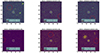 |
Fig. 2. Photometry of the six sources observed with AstroSat/UVIT. Top panel: Zoomed-in view of three RQ sources. Bottom panel: Zoomed-in view of three RL sources. |
Six sources observed with AstroSat/UVIT, using the CaF2 grating centred at 1481 Å (the FUV Band).
2.2. The code: CIGALE v2022.0
The CIGALE v2022.0 code (Yang et al. 2020) is a modular code written in the Python language, the purpose of which is to model the spectra of galaxies from FUV to radio wavelengths. Based on the earlier CIGALE code (Boquien et al. 2019), it can also estimate the physical properties of a galaxy; for example, the star formation rate (SFR), total stellar mass in the galaxy, and contribution of dust luminosity. The code performs the modelling of galaxy spectra through several steps: input processing, input parameter specification, model computation, and analysis.
Firstly, the code checks the input file for input data (e.g. fluxes, errors, redshifts, physical properties), which modules to consider, and their parameter values. After processing and normalising the input data, the code uses this data file to determine the photometric bands or filters to use, among other operations (which are skipped if only model generation is required).
The code first computes the SFH of the galaxy, from which it computes the stellar spectrum and single stellar population (SSP) models. It then models the nebular emission (both line and continuum) caused by Lyman continuum photons and applies dust attenuation and emission models to compute the luminosity contributed or diminished by the dust. Furthermore, it can also model the emission of an AGN, and incorporate the effects of redshift and absorption by the intergalactic medium (IGM).
The SFR can be modelled using several available models; notable among them are the double-exponential SFR, the delayed SFR, the periodic SFR, and so on. It can also read and process SFH from files, using the sfhfromfile module, for modelling arbitrarily complex SFHs. To determine the stellar spectrum, an SSP library is adopted, in addition to the SFH computed in the previous step. The code offers two popular SSP libraries: that of Bruzual & Charlot (2003) (module bc03) and Maraston (2005) (module m2005). Each of them is available for several metallicities, and two initial mass functions (IMFs): Chabrier (2003) and Salpeter (1964).
The nebular emission is important, since it allows one to probe into recent star formation through hydrogen lines and radio continuum. In addition, we can estimate gas metallicity from the metal lines. CIGALE v2022.0 uses nebular templates based on Inoue (2011), which have been generated with CLOUDY 13.01 (Ferland et al. 1998, 2013). These templates depend on the ionisation fraction (U), and metallicity (Z, assumed to be the same as stellar metallicity). The electron density was set at 100 cm−3 and was taken to be a constant, which is a fiducial value assumed for the density. To take into account the absorption of Lyman continuum photons by dust and their escape from the galaxy without ionisation, the nebular emission was down-scaled following Inoue (2011).
The effects of dust attenuation and emission were further applied to these emissions, based on the principle that the energy absorbed by the dust in the UV-NIR range is re-emitted in the mid to far-IR range. The emission of the dust can be modelled, among other ways, by assuming a power law variation of the radiation field intensity (U) with the dust mass (Md):
 (1)
(1)
where α is a parameter of the model.
Attenuation due to dust was calculated following the Calzetti et al. (2000) starburst attenuation curve (module dustatt_modified_staburst), extended with the Leitherer et al. (2002) curve between the Lyman break and 150 nm. The Dale et al. (2014) model (module dale2014) has been implemented for the IR SED of the dust heated by stars, without the AGN component. Continuum and line nebular emission produced in HII regions (module nebular) were considered. Redshifts and the absorption of short wavelength radiation by the IGM (module redshifting) were also taken care of.
Furthermore, the radio synchrotron emission and AGN emission can also be modelled with several available modules in the code. The radio synchrotron emission was modelled by two parameters: a power law slope, α, and a radio-IR correlation, qIR (Helou et al. 1985).
CIGALE v2022.0 is potentially very accurate for the characterisation of galaxies that host AGNs (Best et al. 2023; Pacifici et al. 2023) as it incorporates AGN models that can account for direct AGN light contributions and IR emission arising from AGN heating of the dust. It also predicts the AGN X-ray emission (Yang et al. 2020). The inclusion of AGN models gives CIGALE v2022.0 a significant advantage over other SED fitting codes when fitting the SEDs of galaxies that have a significant AGN contribution. It allows for a more robust estimation of host galaxy parameters, and also a mechanism to identify and classify AGNs within the sample.
The SKIRTOR (module skirtor2016) templates (Stalevski et al. 2012, 2016) are used for AGN emission modelling. SKIRTOR, a clumpy two-phase torus model, considers an anisotropic and constant disc emission. A detailed description of how the SKIRTOR model is being implemented in CIGALE v2022.0 is given in Yang et al. (2020). fracAGN, which is the AGN fraction, is defined as the ratio of the AGN IR emission to the total galaxy IR emission. A dust screen absorption and a grey-body emission are modelled by polar dust component (EB − V). For our work, we adopted the Small Magellanic Cloud extinction curve Prevot et al. (1984). Re-emitted grey-body dust was parameterised with an emissivity index of 1.6 and a temperature of 100 K. For the radio emission modelling, the slope of the power law synchrotron emission related to star formation and that of the power law AGN isotropic radio emission was considered to be 0.8 and 0.7, respectively (Randall et al. 2012; Tiwari 2019). The radio-loudness parameter of AGN was defined as RAGN = Lν,GHz/Lν,2500 A, where Lν,2500 A is the 2500 Å intrinsic disc luminosity measured at a viewing angle of 30°. Moreover, the ratio of the total star-forming IR luminosity (mostly in FIR) and the corresponding radio synchrotron luminosity at 21 cm (1.4 GHz) is defined as qIR.
The code fits the models to the observational data, determines the likelihoods of the models, and uses those likelihoods to estimate the physical properties. Here, the ‘analysis modules’ of the code are used to estimate the physical parameters of interest. The code can utilise two analysis modules to do this; namely, savefluxes, which generates a grid of models and saves the outputs, and pdf_analysis, which, in addition to generating a grid of models, fits them to observational data to estimate physical parameters. The fluxes are observer-dependent and are computed after calculating a given model. The fluxes are obtained in bands by integrating the model spectrum through a corresponding filter.
As was discussed before, SED fitting using CIGALE v2022.0 depends on the input parameter values and choice of models. For our analysis, a delayed SFH model (module sfhdelayed) was applied to build the galaxy component. The model also includes a constant ongoing star formation that is not allowed to be longer than 50Myr. Using the Bruzual & Charlot (2003) SSP templates (module bc03) with the IMF of Salpeter (1964), stellar emission is modelled and metallicity is taken to be equal to the solar value (0.02). The modules and input parameters we used in our analysis are presented in Table 2.
Model parameters for the RL sources (non-HBL+HBL+AstroSat-detected sources) in our sample.
3. Results
As was mentioned before, our RL and RQ samples have five detections in the optical band (u, g, r, i, and z photometric bands from SDSS), four detections in the IR band (W1, W2, W3, and W4 bands from WISE), two UV detections (FUV and NUV bands of GALEX), and one X-ray detection (Chandra/ROSAT/Swift/XMM) with their respective errors. In addition to that, our RL quasars have one radio detection (FIRST 1.4 GHz band). Shen et al. (2011) do not include errors for FIRST detections, so we have assumed an error of 10% in the radio flux. Figure 1 represents the redshift distributions of our final RL and RQ samples.
3.1. Spectral energy distribution modelling using CIGALE v2022.0
Based on our input parameters described in Table 2, we modelled the SEDs of our sources described in Tables A.1 and B.1. We note that the model parameters have been included after extensive parameter studies that followed analysis of previous studies (e.g. Mountrichas et al. 2021, 2022, 2023, 2024a). Figures 3 and 4 represent some example SEDs of the non-HBL RL and RQ sources used in our analysis. Figure 5 represents SEDs of HBL RL and RQ sources and Fig. 6 represents the SEDs of RL and RQ sources observed with AstroSat. For HBL sources and the sources observed with AstroSat, we did not find any X-ray counterpart (see Sect. 2.1). For the SED fitting of our AstroSat sources, we have used a box-car filter centred around 1481 Å as the response function for the CaF2 grating of AstroSat/UVIT FUV observations of these six sources.
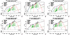 |
Fig. 3. Examples of best-fit SEDs of non-HBL RL quasar sources, constructed using the CIGALE v2022.0 code. Reduced χ2 values calculated by CIGALE v2022.0 code for individual SEDs are provided in the figures. |
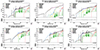 |
Fig. 4. Examples of best-fit SEDs of non-HBL RQ quasar sources, constructed using the CIGALE v2022.0 code. Reduced χ2 values calculated by CIGALE v2022.0 code for individual SEDs are provided in the figures. |
3.2. Extraction of host galaxy properties
From the best-fit SED, we computed the stellar population age, stellar mass, SFR, dust luminosity, and e-folding time of our RL and RQ quasar samples. Figure 7 represents distributions of the host galaxy properties for our RL and RQ sources (non-HBL-SED+HBL+AstroSat-observed). From the best-fit values, we note that the stellar masses are similar for both RL (mean 10.95 ± 0.097 M⊙) and RQ (mean 10.86 ± 0.15 M⊙) quasars, although the stellar masses extend to lower values for RQ quasar host galaxies (see top-left panel of Fig. 7). The luminosity absorbed by dust (for RL the mean is 38.28 ± 0.11 W and for RQ the mean is 38.29 ± 0.14 W), e-folding time (for RL the mean is 2190.7 ± 129.96 Myr and for RQ the mean is 2266.6 ± 249.33 Myr), stellar population age (for RL the mean is 2080.0 ± 246.29 Myr and for RQ the mean is 2850.7 ± 356.69 Myr), and SFR (for RL the mean is 199.15 ± 67.88 M⊙/yr and for RQ the mean is 163.70 ± 67.52 M⊙/yr) are similar for both populations. The mean values are provided in Table 3. We note that the values remain statistically similar for all the sub-classes together and for each sub-class separately; however, some striking features are evident in the stellar mass and SFR properties for our HBL sources that we discuss later.
Mean values of host galaxy properties for RL and RQ quasars in our sample.
To check for the consistency of our modelling, we fitted the SED with the optical+IR+UV, optical+UV, and optical+IR data points. Our results show that excluding the UV leads to an underestimation of the stellar mass, while excluding the IR data affects the best-fit values of the SFR. We note that the UV emission traces young stellar populations and for higher-redshift sources the SDSS u-band might allow observations of radiation emitted by young stars. Hence, it is likely that the absence of UV data might primarily affect SED fitting measurements at lower redshifts. To test for this, we randomly selected RL and RQ quasars at different redshifts and performed the SED analysis with and without UV coverage. We did notice that the effect is stronger at lower redshifts, but the offset (which is always an underestimation of stellar mass) does not exhibit any systematic pattern. Previous studies using X-ray AGNs have found that the absence of UV coverage has a negligible impact on SED analysis, even at low redshifts, in terms of SFR calculations (e.g. Koutoulidis et al. 2022; Mountrichas et al. 2022). Since our UV coverage substantially reduces the sample size, we wish to perform a more extensive analysis of our sources to study host galaxy correlations in future work (Chatterjee et al., in prep.). As was expected, the exclusion of the radio and the X-ray data has almost no effect on the inferred stellar mass or SFR. We are thus confident about the robustness of our fits.
We also note that Mountrichas et al. (2023) found that the SFH parameters are highly degenerate. For example, the degeneracy between stellar age and e-folding time has been discussed. To test for this, we adopted the method proposed by Mountrichas et al. (2023) whereby we include the Hdelta and Dn4000 spectral parameters along with our initial values of other parameters to generate mock fluxes for our sources. We then extracted the best-fit host galaxy parameters from these mock catalogues. We find the best-fit values from the mock catalogues to be statistically identical with our derived best-fit values, validating the robustness of our fits.
To check for the dependence of host galaxy properties with redshift and FWHM (of either the Hβ or Mg II lines), we divided the entire sample into two equally split redshift bins (the lower redshift bin for z ≤ 0.9 and the higher redshift bin for z > 0.9) and three FWHM bins (1500 ≤ FWHM < 5000 km s−1; 5000 ≤ FWHM < 8000 km s−1; and FWHM > 8000 km s−1). We do not find either of the host galaxy properties to be dependent on redshift or FWHM; however, we note that the sample sizes are not significant enough to rule out any such dependence.
To further test for the quality of our fits, we followed the prescription of Mountrichas et al. (2021) by checking the consistency between the Bayesian and best-fit values of host galaxy parameters obtained from CIGALE v2022.0. A large difference between the Bayesian values (which consider the entire parametric grid of all allowed models, with a weight of exp(−χ2/2) for each model) and the best-fit values indicates that a Gaussian probability distribution function cannot correctly reproduce the observed data. As per Mountrichas et al. (2021), we considered the following criteria:  and
and  . We see that in our final sample, 54% of the RL sources and 75% of the RQ ones satisfy these criteria (M21 sub-sample hereafter). We further note that the sources for which the best-fit parameter values of the host galaxy contain large uncertainties are mostly the ones that do not satisfy the above criterion.
In Fig. 8, we plot the M⋆ − SFR relations for our full sample as well as the M21 sub-sample. As is noted, the highest and lowest redshifts of our sources are 1.8 and 0.15, respectively, while the median redshift is about 1.3. The solid lines in all panels represent the main-sequence (MS) relation for three redshifts (.38: blue, 1.33: cyan, and 3.0: brown) from Schreiber et al. (2015). The choice of z = 0.38 comes from the lower limit in redshifts of our sources, barring a few of the Astrosat sources. The top and bottom rows are for the full sample and the M21 sub-sample, respectively. We clearly see that our RL and RQ quasars are off from the Schreiber et al. (2015) relation. In fact, a large number of our quasar sources follow the z = 3.0 MS relation for star-forming galaxies. When we consider our HBL sources (red diamonds), we note a distinct feature. Our HBL RL sources tend to have higher stellar mass with lower SFRs, while for the RQ ones we obtain lower stellar mass with higher SFRs. In addition, we observe a clear hint of a dichotomy in the M⋆ − SFR relation for our RL sources at the higher stellar mass range. The dichotomous trend is more evident for the M21 sub-sample (bottom left panel of Fig. 8).
Simple power law fits to the data show that for our RL sources  and
and  when we consider the full sample and the non-HBL (blue dots in Fig. 8) sample, respectively. For the RQ sources,
  and
and  , respectively, for the full and the non-HBL samples. The trends do not change for the M21 sub-sample. We thus observe that while the mean values of stellar mass and SFR are similar, the average SFR for RL scales higher with stellar mass compared to the RQ population. In a companion paper (Chatterjee et al., in prep), we perform a detailed study of the host galaxy correlations of our sample using the best-fit values derived from the SED modelling.
To check for any trend in the observed MS relation with redshifts, we plot the MS relation in Fig. 9, which are colour-coded by the redshift of the sample. We note that our HBL quasars have a distribution of redshifts, yet the SFR tends to be low for the HBL-RL sources. A somewhat similar trend is also observed for our AstroSat sources. We note that our HBL and AstroSat sources did not have any X-ray counterparts. It was also noted in Chakraborty et al. (2022) that the HBL sample had the lowest Eddington ratio. To test for that, in Fig. 10 we plot the Eddington ratios of our sources as a function of their derived stellar mass. A clear hint of a dichotomy in the Eddington ratio distribution is observed in our RL quasars. We further note that our HBL and AstroSat sources have lower Eddington ratios than our non-HBL sources. Thus, we clearly observe a connection between the SFR and the Eddington ratio. Quasars with lower accretion rates tend to have a lower SFR in their host galaxies, which is a physically plausible scenario, hinting at the unavailability of cold gas in these galaxies.
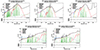 |
Fig. 5. Best-fit SEDs of HBL sources. Reduced χ2 values calculated by CIGALE v2022.0 code for individual SEDS are provided in the figures. Top panel: RL sources. Bottom panel: RQ sources. |
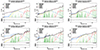 |
Fig. 6. Best-fit SEDs of the sources observed with AstroSat/UVIT without the X-ray data constructed using the CIGALE v2022.0 code. Reduced χ2 values provided by CIGALE v2022.0 for individual SEDs are shown in the figures. Top panel: RL sources. Bottom panel: RQ sources. |
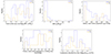 |
Fig. 7. Distributions of host galaxy properties. Top left panel: Solid orange and dashed blue lines denote the histograms of stellar mass (M⋆) for the host galaxies of RQ and RL quasars of the non-HBL+HBL+AstroSat-observed samples. Top middle panel: Same as the top left panel but for the SFR distributions. Top left panel: Same as the top left panel but for the stellar population age distributions. Bottom left panel: Same as the top left panel but for the e-folding time distributions. Bottom right panel: Same as the top left panel but for the dust luminosity distributions. The mean values of the parameters for our RL and RQ sources are provided in Table 3. |
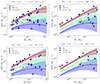 |
Fig. 8. Variation in stellar mass (M⋆) of the host galaxies with their corresponding SFRs. Overplotted solid lines are analytical galaxy MS relations from Schreiber et al. (2015), at different redshifts with corresponding 1-σ uncertainty contours. We note that the highest redshift of our sample is z ∼ 1.8 (see Fig. 1), and thus the z = 3 trend lies outside our sample’s redshift range. The majority of the sources in our sample lie at a significant distance from the galaxy MS and tend to follow the high-redshift (z = 3) trend. In Fig. 9, we have colour-coded our sources with redshifts. Top left panel: For entire RL non-HBL, HBL and AstroSat-observed sources. Top right panel: For entire RQ non-HBL, HBL and AstroSat-observed sources. Bottom left panel: For RL non-HBL, HBL and AstroSat-observed sources that follow the criteria of Mountrichas et al. (2021). Bottom left panel: For RQ non-HBL, HBL and AstroSat-observed sources that follow the criteria of Mountrichas et al. (2021). The observed bimodality in the MS for RL quasars is evident. See Fig. 10 and discussions in Sect. 4. |
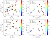 |
Fig. 9. Variation in stellar mass (M⋆) of the host galaxies with their corresponding SFRs for our sources (Fig. 8). The colour bars represent the redshift of each source. Top left panel: For entire RL non-HBL, HBL and AstroSat-observed sources. Top right panel: For entire RQ non-HBL, HBL and AstroSat-observed sources. Bottom left panel: For RL non-HBL, HBL and AstroSat-observed sources that follow the criteria of Mountrichas et al. (2021). Bottom right panel: For RQ non-HBL, HBL and AstroSat-observed sources that follow the criteria of Mountrichas et al. (2021). We do not observe any significant redshift effect in the MS relation. |
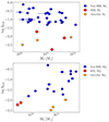 |
Fig. 10. Variation in stellar mass (M⋆) with the Eddington ratio (λEdd) of the central quasar. Top panel: For RL non-HBL, HBL and AstroSat-observed sources. Bottom panel: For RQ non-HBL, HBL and AstroSat-observed sources. See, Fig. 8 and Sect. 4 for discussions. |
3.3. Comparison with SDSS spectra
To highlight the overall agreement of the best-fit CIGALE v2022.0 SED model with the observed data, we overplot the modelled SED with the input photometry from SDSS as well as the SDSS spectrum for the source from the same epoch (see Fig. 11). The best-fit model is quite successful in reproducing multiple features in the observed spectrum, the primary among them being the power law slope of the spectrum. In addition, the intensities of the narrow emission lines can be recovered, albeit with notably higher intensities from the model – a limitation of the finite grid in the ionisation parameter adopted in the CIGALE v2022.0 code. The panels in this figure also highlight the importance of the contribution from the broad emission lines (e.g. C IV, Mg II, and Hβ; see e.g. Panda et al. 2019a; Pozo Nuñez et al. 2023; Panda et al. 2024) and the FeII pseudo-continuum (Panda et al. 2018, 2019b; Pandey et al. 2024) that is composed of multiple overlapping transitions in the spectrum.
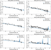 |
Fig. 11. Examples of source spectra from SDSS overplotted with the best-fit SEDs from CIGALE v2022.0 in the optical range. Top panel: For two non-HBL RL quasars from our sample. Middle panel: For two non-HBL RQ quasars from our sample. Bottom left panel: For one HBL RL quasar from our sample. Bottom right panel: For one HBL RQ quasar from our sample. Our SED modelling based on the photometric data is successful in reproducing the quasar spectra. |
The CIGALE v2022.0 modelling does not account for these emission lines given the complexity of reproducing physical conditions for such emitting regions. One also notices minor offsets between the SDSS photometric data and the spectrum. The primary reason behind this is that the photometric data results from the convolution of flux over the broad-band filters. Here, for a given redshift and accounting for the broad emission line contribution (there are other contributors such as the Balmer continuum, and FeII pseudo-continuum; see e.g. Pozo Nuñez et al. 2023; Czerny et al. 2023; Panda et al. 2023, 2024) for the source, the minor discrepancies between the photometric data and spectrum can be mitigated. Nonetheless, the underlying power law continuum of the AGN – the primary ionising source – is reproduced well by our CIGALE v2022.0 models.
3.4. Active galactic nuclei spectral energy distribution simulation
As we are interested in extracting the host galaxy contribution and most of the observed photometric data are dominated by the central quasar, it is important to extract the contribution of the host galaxy to the total luminosity. This is necessary to estimate the contribution of the AGN to the SED in each band. Physically, one would expect that, while the AGN would be dominant in radio, optical, and X-ray bands, the host galaxy contribution would be non-negligible in IR and UV bands. To analyse this, we simulated a pure quasar SED by manually setting the AGN fraction in the IR band, fracAGN = 0.999, using the simulation parameters described in Yang et al. (2020). The contribution of the dominant AGN components in the UV-IR range, the disc, and the torus, is shown in Fig. 12 (top panel). We note that the disc emission dominates the optical range, while the emission from the torus is predominant in the IR. However, if we consider the contribution from all wavelengths, the contribution of the torus is insignificant compared to the disc emission. The relative fractional contribution of the host galaxy to the total flux density, considering the full-physics and the AGN-only simulations, was calculated as:
 |
Fig. 12. Separation of AGN and host galaxy contribution. Top panel: Contribution of the principal AGN Components in the UV–IR range, the accretion disc and the torus, in the total SED of the host galaxy. Bottom panel: Relative contribution of the emission from the host galaxy in the IR–UV part of the SED, following Eq. (2). The emission lines are from the full-physics model and are not present in the AGN-only model. The host galaxy contributes about 50% of the total luminosity at lower wavelengths, and very little at higher wavelengths. See Sects. 3.4 and 4 for more discussions. |
 (2)
(2)
where Fλ, AGN and Fλ, total are the flux densities derived from the AGN-only model (skirtor2016; Stalevski et al. 2016) and the total model (AGN + host galaxy components), respectively. The dependence of fgalaxy on λ is shown in Fig. 12 (bottom panel). As is seen in the figure, we observe a substantial contribution from the host galaxy in the SED. Furthermore, we also checked for changes in the host galaxy properties (from those obtained using all available bands) by systematically removing the X-ray and radio bands from our datasets. We observe that there is little to no change in the host galaxy properties upon making these changes.
4. Discussion
Supermassive BHs at the centre of their host galaxies generate copious amounts of emission from the gravitational potential energy of the accreted material. They can be observed as intense radiation at different wavelengths – for example, X-ray, UV, IR, and radio – which is a characteristic signature of AGNs. The energy released during the accretion process is also an important source of heating the interstellar and intergalactic medium (e.g. Morganti 2017). The observed correlations between host galaxy properties and the central engine (e.g. M–σ relation; Gebhardt et al. 2000; Peterson 2008; Ferrarese & Merritt 2000) suggest a strong connection between the host galaxy and the central AGN. At a broader level, quasar activity plays a role in galaxy evolution and, more generally, structure formation in the Universe (e.g. Brandt & Alexander 2015). A huge volume of work exists in the literature that has probed this connection through spectroscopic studies as well as X-ray and radio imaging (e.g. Berton & Järvelä 2021; Le Fèvre et al. 2019; Giacintucci et al. 2010; Fischer et al. 2019). In our current work, we have constructed the broad-band SEDs of our quasar samples and extracted their host galaxy properties via the modelling of those. In particular, we have tried to address the radio dichotomy issue in quasars by identifying clues in their host galaxy properties; namely, star formation and stellar mass.
The main challenge of this work is in separating the quasar and the host galaxy contributions to the SED. As is discussed in Sect. 3.4, we performed our feasibility study by simulating a quasar spectrum and extracting the host galaxy contribution from there (see Fig. 12). In addition, we performed an alternative analysis to check for consistency. Recently, Jalan et al. (2023) used a large sample of SDSS DR14 quasars to derive an empirical relation between the host galaxy fraction (ratio of the stellar luminosity to the total continuum luminosity) and the total AGN luminosity and redshift, by extracting the host galaxy contribution with stellar templates (e.g. Rakshit & Woo 2018), a power law AGN continuum, iron line templates (see, e.g. Barth et al. 2015; Kovačević et al. 2010), and fitting of emission lines. As our parent sample is SDSS DR7, we used these empirical relations both for redshift (although limited to z ≤ 0.8) and for quasar luminosity. From both the relations, our derived host galaxy fraction is in the range from 20% to 35%.
We have also derived the relative contribution of the host galaxy to the total SED by comparing the relative difference of the SED of a full-physics fitting (i.e. with all components included) with that of an AGN-only fitting in which the AGN-fraction in the total luminosity had been set to unity. This relative contribution (of the host galaxy) is shown in Fig. 12, for the UV–IR range only. We observe that the host galaxy contributes ∼50% of the total luminosity at lower wavelengths in this range, and almost the total luminosity at higher wavelengths (around the FIR range). Thus, our results for the host galaxy contribution appear to be consistent with the estimate of 20% to 35% when integrated over all wavelengths in our sample.
There have been several works on the extraction of host galaxy properties through SED modelling of AGNs (e.g. Mountrichas et al. 2024a; Gadallah 2023; Pouliasis et al. 2022; Koutoulidis et al. 2022; Zou et al. 2022; Zhu et al. 2023; Cutiva-Alvarez et al. 2023; Mountrichas et al. 2021; Yamada et al. 2023). Most of these work involve X-ray bright AGNs, while one study (Cutiva-Alvarez et al. 2023) attempted to model the quasar SED in the NIR/MIR range. Sources in their sample are well beyond our redshift ranges and they find that there is rapid growth (e-folding time: 750–1000 Myrs) of quasars, while the SEDs are degenerate to quasar continuum and starbursts beyond z > 1.6. Mountrichas et al. (2024a) studied X-ray selected AGNs spanning a large range of luminosities and redshifts and found that the shallower slope of the Mstellar − SFR relation in X-ray bright AGN-hosting galaxies implies a smaller amount of star formation in contrast to the galaxy MS. The study shows a slope of 0.21 ± 0.04 for AGN-hosting galaxies and 0.48 ± 0.01 for non-AGN ones in the redshift range of 0.3 < z < 1.0. Similar results are observed in the redshift range of 1.0 < z < 2.0, where the slopes for AGN and non-AGN galaxies are 0.50 ± 0.04 and 0.88 ± 0.02, respectively. As is noted in Sect. 3.2, we observe similar slopes for our quasar host galaxies; however, the results vary once we include the HBL and AstroSat sources. Pouliasis et al. (2022) perform a similar study with X-ray bright AGN and show that AGNs that lie above or within the MS have higher specific accretion rates compared to those below the MS.
In Figs. 8 and 9, we observe a hint of a dichotomy in the M⋆ − SFR relation. As is noted in Chakraborty et al. (2022), the Eddington ratios of the sources in the HBL sample are the lowest and they also exhibit lower SFRs. This correlation has been observed in previous studies, which have explored it using either the Eddington ratio or its proxy, the specific BH accretion rate, across the general AGN population (e.g. Torbaniuk et al. 2021, 2024), different AGN types (such as Sy2, LINERS, composite, and Compton thick AGNs; Mountrichas et al. 2024b), and in relation to X-ray obscuration (e.g. Georgantopoulos et al. 2023; Mountrichas et al. 2024b). In Fig. 10, we further plot the Eddington rates of our quasar sources as a function of their galaxy stellar mass. We observe that the RQ population does not exhibit any notable dichotomy, and it is observed that the Eddington ratios of the quasars follow an increasing trend with the galaxy stellar mass (AstroSat sources deviating from this). The situation changes with the RL population, where we do see a clear dichotomy (at log λEdd = −1.5) between the Eddington ratios of the HBL and the AstroSat sources and the ones of the non-HBL sources.
We note that, across stellar masses, the Eddington ratios remain relatively unchanged (with a slight negative slope). We thus propose that it is likely that the radio jets emanating from low-Eddington ratio systems inhibit star formation in their host galaxies. However, we require further studies with larger samples to test the hypothesis. It is important to note that none of our HBL or AstroSat sources are detected in the X-rays, implying a lower X-ray threshold for these sources. In the future, we wish to perform a wider search, in particular with the eROSITA (Brunner et al. 2022; Merloni et al. 2024) catalogue to discuss the X-ray properties. As was noted before, the main aim of this work is to find clues about the larger RL fraction for optical quasars with broader emission lines that is observed in Chakraborty et al. (2022). Although we do not observe any significant difference in host galaxy properties of RL and RQ quasars when segregated in FWHM, we still observe differences in some host galaxy properties of our sources based on their radio emission. In future, we wish to perform a detailed analysis on the radio SED (Dey et al. 2022) of our RL sources with a wider range of data.
5. Summary
In the previous work of Chakraborty et al. (2022) and Chakraborty & Bhattacharjee (2021), the radio dichotomy of broad-line quasars was studied by looking at their intrinsic differences. The current study aims to examine this dichotomy in the context of host galaxy properties being affected by the presence of radio jets in some systems. For this work, to analyse the host galaxy properties, we compiled a dataset comprising 37 RL quasars and 19 RQ ones (0.15 < z < 1.88) that have at least one broad emission line (either Hβ or Mg II) and modelled the SEDs over a wide range of wavelengths, from the X-ray to the radio, using CIGALE v2022.0. We performed one of the first studies in modelling the broad-band (from X-rays to radio) quasar-hosting galaxy SEDs, classified by their radio emssion. The main results of our investigation can be summarised as follows:
In this work, for the first time we have constructed the multi-wavelength broad-band SED (ranging from X-rays to radio) of optically selected broad-line quasars. We have further classified them as RL and RQ sources and derived their host galaxy properties by modelling their SEDs. In addition to that, we extracted the host galaxy properties of our high broad-line RL and RQ quasars (FWHM > 15 000 kms−1) defined as the HBL sample in Chakraborty et al. (2022) and compared their host galaxy properties with the non-HBL sample. For six of our quasar sources, we obtained FUV data with AstroSat/UVIT. We performed analysis of the AstroSat observations and employed them for the first time for SED analysis using CIGALE v2022.0. We have introduced a box-car filter for fitting the AstroSat FUV data.
-
We obtained host galaxy properties such as stellar mass, SFR, luminosity absorbed by dust, stellar population age, and e-folding time from the SED modelling, and we see that the mean values do not exhibit any difference between the RL and RQ populations.
-
To validate our results, we compared the best-fit model SED we obtained, input photometric data points from Shen et al. (2011), and the SDSS spectrum of the source from the same epoch. The best-fit model for the optical range is quite successful in reproducing multiple features in the observed spectrum by SDSS. We tested for the consistency between the Bayesian and best-fit values of host galaxy parameters from CIGALE v2022.0 using the prescription of Mountrichas et al. (2021) and found that 54% of the RL quasars and 75% of the RQ ones satisfy the prescription.
-
To ensure the fidelity of the extraction of our host galaxy properties, we simulated a pure AGN SED and compared that with the full SED. Our results show that in the UV-IR range about 50–100% of the emission can be reconstructed from the host galaxy, which is adequate for extracting properties such as stellar mass and SFR. We further used the results from Jalan et al. (2023) to extract the host galaxy fraction and our results show that roughly 20-30% of the emission in our sources is due to their host galaxies. The result is consistent with our AGN SED simulation when averaged over all wavelengths.
-
We have obtained the MS relations for our quasars and found that they are far apart from the galaxy MS and tend to follow the high-redshift (z ∼ 3, in Fig. 8) MS relation for star-forming galaxies. We note a dichotomy in the stellar mass -SFR relation for our RL sources, indicating a quenching of star formation. When compared with the Eddington ratios of our sources, we see that there is some connection between quenched star formation and the accretion activity of the central engine, implying a stronger dichotomy in the Eddington ratio-SFR results. We further note that the redshift of our RL and RQ sources does not have any effect on the observed MS relations. We propose to further study host galaxy correlations in a follow-up study (Chatterjee et al., in prep.).
The radio dichotomy problem in quasars is an outstanding question in extra-galactic astronomy. Our previous work Chakraborty et al. (2021, 2022) revealed that the RL fraction increases substantially when quasars are classified based on the width of their emission line. In this study, we performed SED modelling of the host galaxies of our broad-line quasars to check for differences between the RL and RQ populations, as well as the population sampled over their broad-line width. Our analysis shows that although the mean values of the host galaxy parameters of our RL and RQ quasars tend to be similar, we see a difference in the MS relation of our quasars, indicating a difference in the dynamics of the host galaxy modulated by the presence of radio jets in the central engines. We propose to undertake a similar study with larger statistics in the future to have a more conclusive understanding of these effects.
Acknowledgments
The authors wish to thank the anonymous referee whose comments and suggestions have greatly helped in improving the draft. AC wants to thank Evangelos Dimitrios Paspaliaris of INAF – Osservatorio Astrofisico di Arcetri for all his valuable suggestions. SC acknowledges financial support from SERB through the POWER Fellowship (SPF/2022/000084) and the CRG/2020/002064 grant. AC and SC thank Veronique Buat, Denis Burgarella, and Guang Yang for extensive discussion and help with the CIGALE package. SP is supported by the international Gemini Observatory, a program of NSF NOIRLab, which is managed by the Association of Universities for Research in Astronomy (AURA) under a cooperative agreement with the U.S. National Science Foundation, on behalf of the Gemini partnership of Argentina, Brazil, Canada, Chile, the Republic of Korea, and the United States of America. SP also acknowledges the financial support of the Conselho Nacional de Desenvolvimento Cientí-fico e Tecnológico (CNPq) Fellowships 300936/2023-0 and 301628/2024-6. MK acknowledges financial support from SERB through the POWER Fellowship (SPF/2022/000084). SJ wants to thank Joseph E. Postma, UVIT calibration manager, for all his help with the CCDLAB Pipeline. RC thanks ISRO for support under the AstroSat archival data utilization program, SERB for a SURE grant, and Presidency University for support under the Faculty Research and Professional Development Fund (FRPDF). SC and RC acknowledge IUCAA for their hospitality and usage of their facilities through the university associateship program. This work uses UVIT data onboard the AstroSat mission of the Indian Space Research Organization (ISRO), archived at the Indian Space Science Data Center (ISSDC). We thank the payload operations center by the Indian Institute of Astrophysics (IIA) for the initial processing of the UVIT data used in this work.
References
- Abazajian, K. N., Adelman-McCarthy, J. K., Agüeros, M. A., et al. 2009, ApJS, 182, 543 [Google Scholar]
- Archibald, E. N., Dunlop, J. S., Hughes, D. H., et al. 2001, MNRAS, 323, 417 [NASA ADS] [CrossRef] [Google Scholar]
- Baldi, R. D., & Capetti, A. 2008, A&A, 489, 989 [NASA ADS] [CrossRef] [EDP Sciences] [Google Scholar]
- Barth, A. J., Bennert, V. N., Canalizo, G., et al. 2015, ApJS, 217, 26 [NASA ADS] [CrossRef] [Google Scholar]
- Berton, M., & Järvelä, E. 2021, Universe, 7, 188 [NASA ADS] [CrossRef] [Google Scholar]
- Best, P. N., & Heckman, T. M. 2012, MNRAS, 421, 1569 [NASA ADS] [CrossRef] [Google Scholar]
- Best, P. N., Kauffmann, G., Heckman, T. M., et al. 2005, MNRAS, 362, 25 [Google Scholar]
- Best, P. N., Kondapally, R., Williams, W. L., et al. 2023, MNRAS, 523, 1729 [NASA ADS] [CrossRef] [Google Scholar]
- Bianchi, S., Guainazzi, M., Matt, G., Fonseca Bonilla, N., & Ponti, G. 2009, A&A, 495, 421 [NASA ADS] [CrossRef] [EDP Sciences] [Google Scholar]
- Boquien, M., Burgarella, D., Roehlly, Y., et al. 2019, A&A, 622, A103 [NASA ADS] [CrossRef] [EDP Sciences] [Google Scholar]
- Boyle, B. J., & Terlevich, R. J. 1998, MNRAS, 293, L49 [CrossRef] [Google Scholar]
- Brandt, W. N., & Alexander, D. M. 2015, A&ARv, 23, 1 [Google Scholar]
- Brunner, H., Liu, T., Lamer, G., et al. 2022, A&A, 661, A1 [NASA ADS] [CrossRef] [EDP Sciences] [Google Scholar]
- Bruzual, G., & Charlot, S. 2003, MNRAS, 344, 1000 [NASA ADS] [CrossRef] [Google Scholar]
- Calzetti, D., Armus, L., Bohlin, R. C., et al. 2000, ApJ, 533, 682 [NASA ADS] [CrossRef] [Google Scholar]
- Cardelli, J. A., Clayton, G. C., & Mathis, J. S. 1988, ApJ, 329, L33 [NASA ADS] [CrossRef] [Google Scholar]
- Chabrier, G. 2003, PASP, 115, 763 [Google Scholar]
- Chakraborty, A., & Bhattacharjee, A. 2021, Astron. Nachr., 342, 142 [NASA ADS] [CrossRef] [Google Scholar]
- Chakraborty, A., Bhattacharjee, A., & Chatterjee, S. 2021, Galaxies, 9, 74 [Google Scholar]
- Chakraborty, A., Bhattacharjee, A., Brotherton, M. S., et al. 2022, MNRAS, 516, 2824 [NASA ADS] [CrossRef] [Google Scholar]
- Condon, J. J. 1992, ARA&A, 30, 575 [Google Scholar]
- Croft, S., van Breugel, W., de Vries, W., et al. 2006, ApJ, 647, 1040 [NASA ADS] [CrossRef] [Google Scholar]
- Croom, S. M., Richards, G. T., Shanks, T., et al. 2009, MNRAS, 399, 1755 [NASA ADS] [CrossRef] [Google Scholar]
- Cutiva-Alvarez, K. A., Coziol, R., & Torres-Papaqui, J. P. 2023, MNRAS, 521, 3058 [NASA ADS] [CrossRef] [Google Scholar]
- Czerny, B., Panda, S., Prince, R., et al. 2023, A&A, 675, A163 [NASA ADS] [CrossRef] [EDP Sciences] [Google Scholar]
- Dale, D. A., Helou, G., Magdis, G. E., et al. 2014, ApJ, 784, 83 [Google Scholar]
- Dey, S., Goyal, A., Małek, K., et al. 2022, ApJ, 938, 152 [NASA ADS] [CrossRef] [Google Scholar]
- Dunlop, J. S., McLure, R. J., Kukula, M. J., et al. 2003, MNRAS, 340, 1095 [NASA ADS] [CrossRef] [Google Scholar]
- Emonts, B. H. C., Feain, I., Mao, M. Y., et al. 2011, ApJ, 734, L25 [NASA ADS] [CrossRef] [Google Scholar]
- Evans, A. S., Frayer, D. T., Surace, J. A., & Sanders, D. B. 2001, AJ, 121, 1893 [Google Scholar]
- Evans, I. N., Primini, F. A., Glotfelty, K. J., et al. 2010, ApJS, 189, 37 [NASA ADS] [CrossRef] [Google Scholar]
- Falcke, H., Sherwood, W., & Patnaik, A. R. 1996, ApJ, 471, 106 [Google Scholar]
- Ferland, G. J., Korista, K. T., Verner, D. A., et al. 1998, PASP, 110, 761 [Google Scholar]
- Ferland, G. J., Porter, R. L., van Hoof, P. A. M., et al. 2013, Rev. Mex. Astron. Astrofis., 49, 137 [Google Scholar]
- Ferrarese, L., & Merritt, D. 2000, ApJ, 539, L9 [Google Scholar]
- Fischer, T., Smith, K. L., Kraemer, S., et al. 2019, ApJ, 887, 200 [Google Scholar]
- Franceschini, A., Hasinger, G., Miyaji, T., & Malquori, D. 1999, MNRAS, 310, L5 [NASA ADS] [CrossRef] [Google Scholar]
- Gadallah, K. A. K. 2023, MNRAS, 520, 2351 [NASA ADS] [CrossRef] [Google Scholar]
- Gebhardt, K., Bender, R., Bower, G., et al. 2000, ApJ, 539, L13 [Google Scholar]
- Georgantopoulos, I., Pouliasis, E., Mountrichas, G., et al. 2023, A&A, 673, A67 [NASA ADS] [CrossRef] [EDP Sciences] [Google Scholar]
- Giacintucci, S., O’Sullivan, E., Vrtilek, J. M., et al. 2010, in X-ray Astronomy 2009; Present Status, Multi-Wavelength Approach and Future Perspectives, eds. A. Comastri, L. Angelini, M. Cappi, et al. (AIP), AIP Conf. Ser., 1248, 277 [Google Scholar]
- Gürkan, G., Hardcastle, M. J., Best, P. N., et al. 2019, A&A, 622, A11 [NASA ADS] [CrossRef] [EDP Sciences] [Google Scholar]
- Hamilton, T. S. 2010, MNRAS, 407, 2393 [NASA ADS] [CrossRef] [Google Scholar]
- Harrison, C. M. C. 2014, Ph.D. Thesis, Durham University, UK [Google Scholar]
- Heckman, T. M., & Best, P. N. 2014, ARA&A, 52, 589 [Google Scholar]
- Helou, G., Soifer, B. T., & Rowan-Robinson, M. 1985, ApJ, 298, L7 [Google Scholar]
- Herbert, P. D., Jarvis, M. J., Willott, C. J., et al. 2010, MNRAS, 406, 1841 [NASA ADS] [Google Scholar]
- Hopkins, A. M., & Beacom, J. F. 2006, ApJ, 651, 142 [NASA ADS] [CrossRef] [Google Scholar]
- Inoue, A. K. 2011, MNRAS, 415, 2920 [NASA ADS] [CrossRef] [Google Scholar]
- Ivezić, Ž., Menou, K., Knapp, G. R., et al. 2002, AJ, 124, 2364 [CrossRef] [Google Scholar]
- Jalan, P., Rakshit, S., Woo, J.-J., Kotilainen, J., & Stalin, C. S. 2023, MNRAS, 521, L11 [NASA ADS] [CrossRef] [Google Scholar]
- Jiang, L., Fan, X., Ivezić, Ž., et al. 2007, ApJ, 656, 680 [Google Scholar]
- Kalfountzou, E., Trichas, M., Rowan-Robinson, M., et al. 2011, MNRAS, 413, 249 [CrossRef] [Google Scholar]
- Kalfountzou, E., Jarvis, M. J., Bonfield, D. G., & Hardcastle, M. J. 2012, MNRAS, 427, 2401 [NASA ADS] [CrossRef] [Google Scholar]
- Kauffmann, G., Heckman, T. M., Tremonti, C., et al. 2003, MNRAS, 346, 1055 [Google Scholar]
- Kauffmann, G., White, S. D. M., Heckman, T. M., et al. 2004, MNRAS, 353, 713 [Google Scholar]
- Kauffmann, G., Heckman, T. M., & Best, P. N. 2008, MNRAS, 384, 953 [Google Scholar]
- Kellermann, K. I., Sramek, R., Schmidt, M., Shaffer, D. B., & Green, R. 1989, AJ, 98, 1195 [Google Scholar]
- Kimball, A. E., Kellermann, K. I., Condon, J. J., Ivezić, Ž., & Perley, R. A. 2011, ApJ, 739, L29 [NASA ADS] [CrossRef] [Google Scholar]
- Koutoulidis, L., Mountrichas, G., Georgantopoulos, I., Pouliasis, E., & Plionis, M. 2022, A&A, 658, A35 [NASA ADS] [CrossRef] [EDP Sciences] [Google Scholar]
- Kovačević, J., Popović, L. Č., & Dimitrijević, M. S. 2010, ApJS, 189, 15 [Google Scholar]
- Lagos, C. D. P., Padilla, N. D., & Cora, S. A. 2009, MNRAS, 395, 625 [NASA ADS] [CrossRef] [Google Scholar]
- Laor, A., & Behar, E. 2008, MNRAS, 390, 847 [NASA ADS] [CrossRef] [Google Scholar]
- Laor, A., Fiore, F., Elvis, M., Wilkes, B. J., & McDowell, J. C. 1997, ApJ, 477, 93 [Google Scholar]
- Le Fèvre, O., Lemaux, B. C., Nakajima, K., et al. 2019, A&A, 625, A51 [NASA ADS] [CrossRef] [EDP Sciences] [Google Scholar]
- Leitherer, C., Calzetti, D., & Martins, L. 2002, P., 574, 114 [Google Scholar]
- Madau, P., Ferguson, H. C., Dickinson, M. E., et al. 1996, MNRAS, 283, 1388 [Google Scholar]
- Maraston, C. 2005, MNRAS, 362, 799 [NASA ADS] [CrossRef] [Google Scholar]
- Martin, D. C., Fanson, J., Schiminovich, D., et al. 2005, ApJ, 619, L1 [Google Scholar]
- Marziani, P., Sniegowska, M., Panda, S., et al. 2021, Am. Astron. Soc. Meeting Abstr., 53, 337.03 [Google Scholar]
- Marziani, P., Panda, S., Deconto Machado, A., & Del Olmo, A. 2023, Galaxies, 11, 52 [NASA ADS] [CrossRef] [Google Scholar]
- McLure, R. J., & Dunlop, J. S. 2001, MNRAS, 321, 515 [NASA ADS] [CrossRef] [Google Scholar]
- McLure, R. J., & Dunlop, J. S. 2004, MNRAS, 352, 1390 [NASA ADS] [CrossRef] [Google Scholar]
- McLure, R. J., & Jarvis, M. J. 2004, MNRAS, 353, L45 [NASA ADS] [CrossRef] [Google Scholar]
- Merloni, A., Lamer, G., Liu, T., et al. 2024, A&A, 682, A34 [NASA ADS] [CrossRef] [EDP Sciences] [Google Scholar]
- Miller, L., Peacock, J. A., & Mead, A. R. G. 1990, MNRAS, 244, 207 [NASA ADS] [Google Scholar]
- Miller, P., Rawlings, S., & Saunders, R. 1993, MNRAS, 263, 425 [NASA ADS] [Google Scholar]
- Morganti, R. 2017, Nat. Astron., 1, 596 [Google Scholar]
- Mountrichas, G., Buat, V., Yang, G., et al. 2021, A&A, 653, A74 [NASA ADS] [CrossRef] [EDP Sciences] [Google Scholar]
- Mountrichas, G., Masoura, V. A., Xilouris, E. M., et al. 2022, A&A, 661, A108 [NASA ADS] [CrossRef] [EDP Sciences] [Google Scholar]
- Mountrichas, G., Yang, G., Buat, V., et al. 2023, A&A, 675, A137 [NASA ADS] [CrossRef] [EDP Sciences] [Google Scholar]
- Mountrichas, G., Masoura, V. A., Corral, A., & Carrera, F. J. 2024a, A&A, 683, A143 [NASA ADS] [CrossRef] [EDP Sciences] [Google Scholar]
- Mountrichas, G., Viitanen, A., Carrera, F. J., et al. 2024b, A&A, 683, A172 [NASA ADS] [CrossRef] [EDP Sciences] [Google Scholar]
- Netzer, H. 2015, ARA&A, 53, 365 [Google Scholar]
- Pacifici, C., Iyer, K. G., Mobasher, B., et al. 2023, ApJ, 944, 141 [NASA ADS] [CrossRef] [Google Scholar]
- Page, M. J., Stevens, J. A., Mittaz, J. P. D., & Carrera, F. J. 2001, Science, 294, 2516 [NASA ADS] [CrossRef] [Google Scholar]
- Panda, S., Czerny, B., Adhikari, T. P., et al. 2018, ApJ, 866, 115 [CrossRef] [Google Scholar]
- Panda, S., Martínez-Aldama, M. L., & Zajaček, M. 2019a, Front. Astron. Space Sci., 6, 75 [NASA ADS] [CrossRef] [Google Scholar]
- Panda, S., Marziani, P., & Czerny, B. 2019b, ApJ, 882, 79 [NASA ADS] [CrossRef] [Google Scholar]
- Panda, S., Marziani, P., Czerny, B., Rodríguez-Ardila, A., & Pozo Nuñez, F. 2023, Universe, 9, 492 [NASA ADS] [CrossRef] [Google Scholar]
- Panda, S., Kozłowski, S., Gromadzki, M., et al. 2024, ApJS, 272, 11 [NASA ADS] [CrossRef] [Google Scholar]
- Pandey, A., Martínez-Aldama, M. L., Czerny, B., Panda, S., & Zajaček, M. 2024, arXiv e-prints [arXiv:2401.18052] [Google Scholar]
- Peterson, B. M. 2008, New Astron. Rev., 52, 240 [Google Scholar]
- Postma, J. E., & Leahy, D. 2017, PASP, 129, 115002 [Google Scholar]
- Pouliasis, E., Mountrichas, G., Georgantopoulos, I., et al. 2022, A&A, 667, A56 [NASA ADS] [CrossRef] [EDP Sciences] [Google Scholar]
- Pozo Nuñez, F., Bruckmann, C., Deesamutara, S., et al. 2023, MNRAS, 522, 2002 [CrossRef] [Google Scholar]
- Prevot, M. L., Lequeux, J., Maurice, E., Prevot, L., & Rocca-Volmerange, B. 1984, A&A, 132, 389 [Google Scholar]
- Rafter, S. E., Crenshaw, D. M., & Wiita, P. J. 2011, AJ, 141, 85 [NASA ADS] [CrossRef] [Google Scholar]
- Rakshit, S., & Woo, J.-H. 2018, ApJ, 865, 5 [Google Scholar]
- Randall, K. E., Hopkins, A. M., Norris, R. P., et al. 2012, MNRAS, 421, 1644 [NASA ADS] [CrossRef] [Google Scholar]
- Reuland, M., Rottgering, H., Van Breugel, W., & De Breuck, C. 2004, MNRAS, 353, 377 [CrossRef] [Google Scholar]
- Richards, G. T., & Kratzer, R. 2014, Am. Astron. Soc. Meeting Abstr., 223, 150.35 [Google Scholar]
- Salpeter, E. E. 1964, ApJ, 140, 796 [NASA ADS] [CrossRef] [Google Scholar]
- Sánchez, S. F., Jahnke, K., Wisotzki, L., et al. 2004, ApJ, 614, 586 [CrossRef] [Google Scholar]
- Sandage, A. 1965, ApJ, 141, 1560 [NASA ADS] [CrossRef] [Google Scholar]
- Schartmann, M., Meisenheimer, K., Camenzind, M., Wolf, S., & Henning, T. 2005, A&A, 437, 861 [NASA ADS] [CrossRef] [EDP Sciences] [Google Scholar]
- Schmidt, M. 1963, Nature, 197, 1040 [Google Scholar]
- Schmidt, M., & Green, R. F. 1983, ApJ, 269, 352 [NASA ADS] [CrossRef] [Google Scholar]
- Schreiber, C., Pannella, M., Elbaz, D., et al. 2015, A&A, 575, A74 [NASA ADS] [CrossRef] [EDP Sciences] [Google Scholar]
- Scoville, N. Z., Frayer, D. T., Schinnerer, E., & Christopher, M. 2003, ApJ, 585, L105 [NASA ADS] [CrossRef] [Google Scholar]
- Shen, Y., Greene, J. E., Strauss, M. A., Richards, G. T., & Schneider, D. P. 2008, ApJ, 680, 169 [Google Scholar]
- Shen, Y., Richards, G. T., Strauss, M. A., et al. 2011, ApJS, 194, 45 [Google Scholar]
- Sikora, M., Stawarz, Ł., & Lasota, J.-P. 2007, ApJ, 658, 815 [NASA ADS] [CrossRef] [Google Scholar]
- Silk, J., & Nusser, A. 2010, ApJ, 725, 556 [NASA ADS] [CrossRef] [Google Scholar]
- Skrutskie, M. F., Cutri, R. M., Stiening, R., et al. 2006, AJ, 131, 1163 [NASA ADS] [CrossRef] [Google Scholar]
- Stalevski, M., Fritz, J., Baes, M., Nakos, T., & Popović, L. Č. 2012, MNRAS, 420, 2756 [Google Scholar]
- Stalevski, M., Ricci, C., Ueda, Y., et al. 2016, MNRAS, 458, 2288 [Google Scholar]
- Stevens, J. A., Page, M. J., Ivison, R. J., et al. 2005, MNRAS, 360, 610 [CrossRef] [Google Scholar]
- Strittmatter, P. A., Hill, P., Pauliny-Toth, I. I. K., Steppe, H., & Witzel, A. 1980, A&A, 88, L12 [NASA ADS] [Google Scholar]
- Svoboda, J., Guainazzi, M., & Merloni, A. 2017, A&A, 603, A127 [NASA ADS] [CrossRef] [EDP Sciences] [Google Scholar]
- Tadhunter, C., Robinson, T. G., González Delgado, R. M., Wills, K., & Morganti, R. 2005, MNRAS, 356, 480 [CrossRef] [Google Scholar]
- Tandon, S. N., Postma, J., Joseph, P., et al. 2020, AJ, 159, 158 [Google Scholar]
- Tiwari, P. 2019, RAA, 19, 096 [NASA ADS] [Google Scholar]
- Torbaniuk, O., Paolillo, M., Carrera, F., et al. 2021, MNRAS, 506, 2619 [NASA ADS] [CrossRef] [Google Scholar]
- Torbaniuk, O., Paolillo, M., D’Abrusco, R., et al. 2024, MNRAS, 527, 12091 [Google Scholar]
- Trichas, M., Rowan-Robinson, M., Georgakakis, A., et al. 2010, MNRAS, 405, 2243 [NASA ADS] [Google Scholar]
- Trichas, M., Green, P. J., Silverman, J. D., et al. 2012, ApJS, 200, 17 [CrossRef] [Google Scholar]
- Truemper, J. 1982, Adv. Space Res., 2, 241 [Google Scholar]
- Tueller, J., Mushotzky, R. F., Barthelmy, S., et al. 2008, ApJ, 681, 113 [NASA ADS] [CrossRef] [Google Scholar]
- Walter, F., Carilli, C., Bertoldi, F., et al. 2004, ApJ, 615, L17 [NASA ADS] [CrossRef] [Google Scholar]
- White, R. L., Helfand, D. J., Becker, R. H., Glikman, E., & de Vries, W. 2007, ApJ, 654, 99 [Google Scholar]
- Wright, E. L., Eisenhardt, P. R. M., Mainzer, A. K., et al. 2010, AJ, 140, 1868 [Google Scholar]
- Yamada, S., Ueda, Y., Herrera-Endoqui, M., et al. 2023, ApJS, 265, 37 [NASA ADS] [CrossRef] [Google Scholar]
- Yang, G., Boquien, M., Buat, V., et al. 2020, MNRAS, 491, 740 [Google Scholar]
- Yang, G., Boquien, M., Brandt, W. N., et al. 2022, ApJ, 927, 192 [NASA ADS] [CrossRef] [Google Scholar]
- York, D. G., Adelman, J., Anderson, J. E., Jr, et al. 2000, AJ, 120, 1579 [Google Scholar]
- Zamfir, S., Sulentic, J. W., & Marziani, P. 2008, MNRAS, 387, 856 [NASA ADS] [CrossRef] [Google Scholar]
- Zhu, S., Brandt, W. N., Zou, F., et al. 2023, MNRAS, 522, 3506 [NASA ADS] [CrossRef] [Google Scholar]
- Zou, F., Brandt, W. N., Chen, C.-T., et al. 2022, ApJS, 262, 15 [NASA ADS] [CrossRef] [Google Scholar]
Appendix
Data of RL quasars
Appendix
Data of RQ quasars
All Tables
Six sources observed with AstroSat/UVIT, using the CaF2 grating centred at 1481 Å (the FUV Band).
Model parameters for the RL sources (non-HBL+HBL+AstroSat-detected sources) in our sample.
All Figures
|
Fig. 1. Histograms of redshift for the non-HBL+HBL+AstroSat-observed RL (dashed blue) and RQ (solid orange) sources in our sample. Our datasets are described in Sect. 2.1. |
| In the text | |
|
Fig. 2. Photometry of the six sources observed with AstroSat/UVIT. Top panel: Zoomed-in view of three RQ sources. Bottom panel: Zoomed-in view of three RL sources. |
| In the text | |
|
Fig. 3. Examples of best-fit SEDs of non-HBL RL quasar sources, constructed using the CIGALE v2022.0 code. Reduced χ2 values calculated by CIGALE v2022.0 code for individual SEDs are provided in the figures. |
| In the text | |
|
Fig. 4. Examples of best-fit SEDs of non-HBL RQ quasar sources, constructed using the CIGALE v2022.0 code. Reduced χ2 values calculated by CIGALE v2022.0 code for individual SEDs are provided in the figures. |
| In the text | |
|
Fig. 5. Best-fit SEDs of HBL sources. Reduced χ2 values calculated by CIGALE v2022.0 code for individual SEDS are provided in the figures. Top panel: RL sources. Bottom panel: RQ sources. |
| In the text | |
|
Fig. 6. Best-fit SEDs of the sources observed with AstroSat/UVIT without the X-ray data constructed using the CIGALE v2022.0 code. Reduced χ2 values provided by CIGALE v2022.0 for individual SEDs are shown in the figures. Top panel: RL sources. Bottom panel: RQ sources. |
| In the text | |
|
Fig. 7. Distributions of host galaxy properties. Top left panel: Solid orange and dashed blue lines denote the histograms of stellar mass (M⋆) for the host galaxies of RQ and RL quasars of the non-HBL+HBL+AstroSat-observed samples. Top middle panel: Same as the top left panel but for the SFR distributions. Top left panel: Same as the top left panel but for the stellar population age distributions. Bottom left panel: Same as the top left panel but for the e-folding time distributions. Bottom right panel: Same as the top left panel but for the dust luminosity distributions. The mean values of the parameters for our RL and RQ sources are provided in Table 3. |
| In the text | |
|
Fig. 8. Variation in stellar mass (M⋆) of the host galaxies with their corresponding SFRs. Overplotted solid lines are analytical galaxy MS relations from Schreiber et al. (2015), at different redshifts with corresponding 1-σ uncertainty contours. We note that the highest redshift of our sample is z ∼ 1.8 (see Fig. 1), and thus the z = 3 trend lies outside our sample’s redshift range. The majority of the sources in our sample lie at a significant distance from the galaxy MS and tend to follow the high-redshift (z = 3) trend. In Fig. 9, we have colour-coded our sources with redshifts. Top left panel: For entire RL non-HBL, HBL and AstroSat-observed sources. Top right panel: For entire RQ non-HBL, HBL and AstroSat-observed sources. Bottom left panel: For RL non-HBL, HBL and AstroSat-observed sources that follow the criteria of Mountrichas et al. (2021). Bottom left panel: For RQ non-HBL, HBL and AstroSat-observed sources that follow the criteria of Mountrichas et al. (2021). The observed bimodality in the MS for RL quasars is evident. See Fig. 10 and discussions in Sect. 4. |
| In the text | |
|
Fig. 9. Variation in stellar mass (M⋆) of the host galaxies with their corresponding SFRs for our sources (Fig. 8). The colour bars represent the redshift of each source. Top left panel: For entire RL non-HBL, HBL and AstroSat-observed sources. Top right panel: For entire RQ non-HBL, HBL and AstroSat-observed sources. Bottom left panel: For RL non-HBL, HBL and AstroSat-observed sources that follow the criteria of Mountrichas et al. (2021). Bottom right panel: For RQ non-HBL, HBL and AstroSat-observed sources that follow the criteria of Mountrichas et al. (2021). We do not observe any significant redshift effect in the MS relation. |
| In the text | |
|
Fig. 10. Variation in stellar mass (M⋆) with the Eddington ratio (λEdd) of the central quasar. Top panel: For RL non-HBL, HBL and AstroSat-observed sources. Bottom panel: For RQ non-HBL, HBL and AstroSat-observed sources. See, Fig. 8 and Sect. 4 for discussions. |
| In the text | |
|
Fig. 11. Examples of source spectra from SDSS overplotted with the best-fit SEDs from CIGALE v2022.0 in the optical range. Top panel: For two non-HBL RL quasars from our sample. Middle panel: For two non-HBL RQ quasars from our sample. Bottom left panel: For one HBL RL quasar from our sample. Bottom right panel: For one HBL RQ quasar from our sample. Our SED modelling based on the photometric data is successful in reproducing the quasar spectra. |
| In the text | |
|
Fig. 12. Separation of AGN and host galaxy contribution. Top panel: Contribution of the principal AGN Components in the UV–IR range, the accretion disc and the torus, in the total SED of the host galaxy. Bottom panel: Relative contribution of the emission from the host galaxy in the IR–UV part of the SED, following Eq. (2). The emission lines are from the full-physics model and are not present in the AGN-only model. The host galaxy contributes about 50% of the total luminosity at lower wavelengths, and very little at higher wavelengths. See Sects. 3.4 and 4 for more discussions. |
| In the text | |
Current usage metrics show cumulative count of Article Views (full-text article views including HTML views, PDF and ePub downloads, according to the available data) and Abstracts Views on Vision4Press platform.
Data correspond to usage on the plateform after 2015. The current usage metrics is available 48-96 hours after online publication and is updated daily on week days.
Initial download of the metrics may take a while.