| Issue |
A&A
Volume 694, February 2025
|
|
|---|---|---|
| Article Number | A315 | |
| Number of page(s) | 14 | |
| Section | The Sun and the Heliosphere | |
| DOI | https://doi.org/10.1051/0004-6361/202451706 | |
| Published online | 24 February 2025 | |
Sun-as-a-star analysis of simulated solar flares
1
School of Astronomy and Space Science, Nanjing University, 163 Xianlin Road, Nanjing 210023, PR China
2
Key Laboratory for Modern Astronomy and Astrophysics (Nanjing University), Ministry of Education, Nanjing 210023, 163 Xianlin Road, PR China
3
Institute for Solar Physics, Dept. of Astronomy, Stockholm University, AlbaNova University Centre, SE-106 91 Stockholm, Sweden
⋆ Corresponding authors; This email address is being protected from spambots. You need JavaScript enabled to view it.
, This email address is being protected from spambots. You need JavaScript enabled to view it.
Received:
29
July
2024
Accepted:
26
December
2024
Abstract
Context. Stellar flares have an impact on habitable planets. To relate the observations of the Sun with those of stars, one needs to use a Sun-as-a-star analysis, that is, to degrade the resolution of the Sun to a single point. With the data of the Sun-as-a-star observations, a simulation of solar flares is required to provide a systemic clue for the Sun-as-a-star study.
Aims. We aim to explore how the Sun-as-a-star spectrum varies with the flare magnitude and location based on a grid of solar flare models.
Methods. Using 1D radiative hydrodynamics modeling and multi-thread flare assumption, we obtained the spectrum of a typical flare with an enhancement of chromospheric lines.
Results. The Sun-as-a-star spectrum of the Hα line shows enhanced and shifted components, which are highly dependent on the flare magnitude and location. The equivalent width ΔEW is a good indicator of energy release. The bisector method can be used to diagnose the sign of the line-of-sight velocity in the flaring atmosphere. For both Hα and Hβ lines, the Sun-as-a-star spectrum of a limb flare tends to be wider and shows a dip in the line center. In particular, we propose two quantities to diagnose the magnitude and location of the stellar flares. Besides this, caution must be taken when calculating the radiation energy, since the astrophysical flux-to-energy conversion ratio is dependent on the flare location.
Key words: line: profiles / radiative transfer / Sun: flares / stars: flare
© The Authors 2025
 Open Access article, published by EDP Sciences, under the terms of the Creative Commons Attribution License (https://creativecommons.org/licenses/by/4.0), which permits unrestricted use, distribution, and reproduction in any medium, provided the original work is properly cited.
This article is published in open access under the Subscribe to Open model. This email address is being protected from spambots. You need JavaScript enabled to view it. to support open access publication.
1. Introduction
In order to search for habitable planets, it is necessary to learn the change in the interplanetary space environment that originated from the hosting star. A star with intense and frequent activities can strongly influence the space weather; such activities have a significant impact on the creation and maintenance of life on planets. Stellar flares are a common type of stellar activity, which release a large amount of energy in a short period (Kowalski 2024). Flares are thought to originate from magnetic reconnections and are sometimes accompanied by coronal mass ejections (CMEs) and energetic particles, which can hazardously change the space weather (Pulkkinen 2007; Tsurutani et al. 2003). During flares, energy is released from the magnetic field in the upper atmosphere (Parker 1963; Shibata & Tanuma 2001; Shibata & Magara 2011), which is partly converted to a radiation enhancement observed in multi-spectral windows such as the radio, optical, ultraviolet, X-rays, and so on. For solar flares, the released energy is typically 1029–1033 erg. In other stars, the total energy can reach up to 1036 erg (Maehara et al. 2012). However, there is recent a debate about whether the total flare energy can be derived from the assumption of black-body radiation or hydrogen recombination continuum. The latter would lower the estimated total energy by one order of magnitude (Simões et al. 2024).
Since stars are too distant to be observed with sufficient spatial resolution, as the Sun has, determining the flare level and even its location on the stars is a significant challenge. Therefore, one usually resorts to observations and modeling of the Sun. Studying the Sun provides a bridge to understanding what could happen on other stars – especially solar-type stars (Notsu et al. 2013) – since all transient events on the Sun may also occur in other types of stars (Haisch et al. 1991).
To relate the observations of the Sun with those of stars, one has to degrade the resolution of the Sun to a single point, that is, integrate the observables over the full disk of the Sun. The method is called the Sun-as-a-star analysis (e.g. Woods et al. 2004; Kretzschmar 2011; Pietrow & Pastor Yabar 2024). This method is widely used in determining the long-period variation of the total solar irradiance (TSI) (Livingston et al. 2007; Criscuoli et al. 2023; Zills et al. 2024). Today, the Sun-as-a-star method is also used for detecting short-period events such as solar flares and filament eruptions (Otsu et al. 2022; Namekata et al. 2022a; Xu et al. 2022; Pietrow et al. 2024a).
For solar flares, the flaring region is too small compared with the whole solar disk, making it very difficult to directly see the flare signals from the optical spectra. A practical way to extract the flare signals is to study the Sun-as-a-star spectrum subtracted by the pre-flare one. Namekata et al. (2022a) calculated the pre-flare-subtracted Hα spectra taken by the Solar Dynamics Doppler Imager, from which the velocity and line width are obtained. Otsu et al. (2022), Otsu & Asai (2024) used the same instrument and method to analyze several flares, filament eruptions, and prominence eruptions. They suggest that the different characteristics in the Sun-as-a-star profiles can be evidence of different kinds of activities.
Furthermore, the result of Otsu et al. (2022) suggests that the Hα line emission is related to the location of the flare, showing a center-to-limb variation (CLV). The CLV effect has been proven to be significant in the quiet-Sun spectrum (Pietrow et al. 2023; Pietrow & Pastor Yabar 2024). Such an effect is even more conspicuous when a flare occurs, in other words, two identical flares can result in very different Sun-as-a-star spectra if one is located at the disk center and the other is at the disk limb. By considering the CLV effect on flare observations, Woods et al. (2006) used the traditional limb-darkening formula to obtain the ratio of the TSI to the GOES X-ray flare energy as a function of the flare location. Although there have been some previous studies, the CLV effect in solar or stellar flares is still poorly understood and requires further in-depth research, as indicated by Notsu et al. (2024). One may notice that the previous studies are mostly based on observations, and those based on simulations are still lacking. By comparison, simulations are more illustrative in revealing the CLV effect in dependence on key parameters like the flare magnitudes and locations, thus providing a clue to diagnosing stellar flares.
In this paper, we introduce a model to calculate the Sun-as-a-star spectrum of chromospheric lines during a flare. A specific parameter study on the Sun-as-a-star spectrum is presented. The two key parameters in our model include the flare magnitude and location. In Sect. 2, we introduce the model used in our work. We show the result in Sect. 3, and we compare it to observations in Sect. 4. Finally, we summarize our results in Sect. 5.
2. Method
Observations with high spatial resolution have shown that flares are not composed of a single loop (Aschwanden & Alexander 2001) but a series of loops. To be realistic, a multi-thread flare simulation is suggested (Warren 2006; Rubio da Costa et al. 2016; Kowalski et al. 2017). The principle of multi-thread simulation is that the foot points of flare loops brighten consecutively as the magnetic reconnection proceeds and all the brightened foot points contribute to the total flare radiation. We adopt such a model in this work. We first simulated the spectrum of a flaring loop, which is regarded as a single thread. Then, we calculated the multi-thread spectrum based on the result of the single thread.
2.1. Simulation of a single thread
The RADYN code is a one-dimensional radiative hydrodynamic code based on a plane-parallel atmosphere (Carlsson & Stein 1992, 1995, 1997, 2002). It is now used more often to calculate the atmospheric response under flare conditions (Allred et al. 2015). Solar flares are assumed to be caused by nonthermal electrons, which are produced by magnetic reconnection in the corona. The electrons lose their energy by interacting with ambient particles through coulomb collisions, leading to the heating of the atmosphere in the meantime. In our simulation, the initial atmosphere is based on the VAL3C model, with a 20 Mm flare loop. We only simulated one leg of a semicircular loop from the photosphere to the corona (10 Mm). A nonthermal electron beam is injected from the loop top and travels downward along the loop. For each simulation thread, the energy flux of the electron beam linearly increases with time in the first 10 s, maintains the maximum value for 10 s, and then linearly decreases for the next 10 s. After that, the atmosphere continues to evolve with no heating for the last 30 s. The total simulation time for a single thread is thus 60 s, which is on the same order as in Rubio da Costa et al. (2016). We assume that the electrons follow a power-law distribution, with a fixed cut-off energy of Ec = 25 keV and a fixed spectral index of δ = 3. These two parameters change the penetration depth of the beam, and we fixed their values to some typical ones similar to those seen in previous flare simulations (Kerr et al. 2019; Hong et al. 2022; Yu et al. 2023). The peak energy flux Fpeak is a key parameter in flare simulations. Here, we take ten values from 1010 erg s−1 cm−2 to 1011 erg s−1 cm−2 for Fpeak, so as to cover different energy magnitudes of flares (hereafter noted as 1–10). The quadricircular loop is 10 Mm in length and the initial atmosphere is adopted to be the quiet-Sun model with a loop-top temperature of 1 MK.
In the simulation, we calculated the emergent intensity for five positions on the solar disk denoted by the cosine of the heliocentric angle μ ≡ cos θ. The values of μ are fixed at 0.047, 0.231, 0.500, 0.769, and 0.953, from the solar limb to the disk center. We ran the above single-thread simulation for 60 s and saved the snapshot every 1 s.
The spectral lines in RADYN are all calculated with the assumption of complete frequency redistribution, which is inaccurate for strong resonance lines such as Ca II K&H. So, we only took the Hα and Hβ lines from RADYN outputs. We then fed the simulation output to RH 1.5D (Pereira & Uitenbroek 2015) to recalculate the spectral lines (assuming partial frequency redistribution) and continua with different flare locations μ and a different electron beam flux Fpeak. We took all the Ca II K&H lines and continua from here. Thus, for each value of Fpeak, we obtain a three-dimensional data matrix for the emergent intensity as I(μ, λ, t).
2.2. Multi-thread model
Qiu & Longcope (2016) proposed two modes of multi-thread simulation: amplitude modulation and frequency modulation. Amplitude modulation modifies the intensity of each thread, while the time interval between two consecutive threads is constant. Frequency modulation means that the threads are all the same, but their occurrence rate changes with time. For both modulation types, every single loop brightens independently and does not interact with the adjacent loop.
Given a flare location μ and electron beam flux Fpeak, we used the multi-thread simulation with frequency modulation. At a given time t, the flare loops in the flare region are at different heating stages. We introduce an occurrence rate P(t) to denote the gradient of the cumulative fraction of loops that have started flaring. Thus, P(t)dt is equal to the percentage of the flare loops that start being heated at the time from t to t + dt, with  , where T is the total time when the heating of different threads is initiated in the multi-thread model. The average intensity of the flare region is then expressed as
 (1)
(1)
We note that the time range of a single thread I(μ, λ, t) is 0 s ≤t ≤ 60 s, so when t < 0 s or t > 60 s, we used the values at the boundary. Following Qiu & Longcope (2016), P(t) is set to be a two-half-Gaussian profile,
![Mathematical equation: $$ \begin{aligned} P(t) = {\left\{ \begin{array}{ll} \displaystyle C \, \mathrm{exp} \left[-\frac{(t-t_0)^2}{2\tau _0^2}\right]&0< t < t_0 \\ \displaystyle C \, \mathrm{exp} \left[-\frac{(t-t_0)^2}{18\tau _0^2}\right]&t_0 <t < T \\ \end{array}\right.}, \end{aligned} $$](/articles/aa/full_html/2025/02/aa51706-24/aa51706-24-eq3.gif) (2)
(2)
with a quick growth and a long decay, where C is the normalizing factor. Here, we take T = 1200 s, t0 = 200 s, and τ0 = 50 s; the normalizing factor C is equal to  . These parameters are set arbitrarily so that the shape of the soft X-ray flux curve in our model (Fig. 1) is similar to that in a typical solar flare (e.g., Namekata et al. 2022a). Other sets of P(t) will definitely change the light curve, but they will not qualitatively change the results. As the heating of each thread lasts 60 s, the total simulation time would be 1260 s in the multi-thread model.
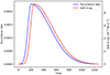 |
Fig. 1. Occurrence rate P(t) (blue) and GOES 1–8 Å flux when Fpeak = 5 (red) as a function of time. The X-ray synthetic method is introduced in Sect. 4.1. |
2.3. Sun-as-a-star analysis
As is well known, for an unresolved star we are actually observing its astrophysical flux F (which is equivalent to the intensity averaged over the apparent stellar disk  ) instead of the specific intensity. For the quiet Sun (t = 0 s in our simulation), the astrophysical flux is calculated as
 (3)
(3)
where we used the Gauss-Legendre quadrature, and the weight wn is 0.118, 0.239, 0.284, 0.239, and 0.118 for the five μn values listed in Sect. 2.1.
Compared to the whole disk, the flare is restricted to a small region where μ does not change much. We assume that the remainder of the disk is still well-represented by the quiet-Sun model. Then, for a given flare location μ, we can write the difference in astrophysical flux as
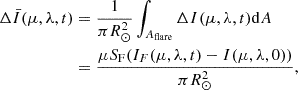 (4)
(4)
where the apparent area A is given by μSF, and the flaring area SF is assumed to be 1.5 × 1018cm2, which is a typical value of the flare ribbon area (estimated from Zhou et al. 2022). After normalizing this quantity by the quiet-Sun flux at the far wing (near-continuum) of each line, we can obtain the so-called Sun-as-a-star spectrum ΔS as defined in Namekata et al. (2022a):
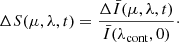 (5)
(5)
We note that the astrophysical flux in a flare case is  . After that, we constructed a grid of 50 flare models with ten different flare magnitudes and five different flare locations. It should be pointed out that in the above method, the following assumptions have been made:
-
The rotation of the Sun is neglected. This might affect the Doppler shift of the Sun-as-a-star spectrum ΔS when the flare occurs near the east or west limb.
-
The plane-parallel assumption means that we do not consider the orientation of the loops. The loop can be thought of as vertical to the surface, and the atmosphere is always extended in the x-y plane. We did not consider whether the flaring atmosphere is embedded in a variety of different initial atmospheres, as suggested in previous observations (Pietrow et al. 2024b).
-
The “halo” of the flare is not included in our 1D simulation, which can also play a role in contributing to the flare spectra (Namekata et al. 2022a).
-
The parameters of the nonthermal electron beam and the initial atmosphere are fixed in each multi-thread case. However, it is believed that beam injection sites can be localized within the flare ribbon (Druett et al. 2017; Osborne & Fletcher 2022; Polito et al. 2023).
-
We only focus on the flare ribbons as a simple model. Associated filament eruptions or CMEs are thus not included. However, as indicated by Otsu et al. (2022), the Doppler shift of the filament can be a very prominent characteristic of the Sun-as-a-star spectrum.
3. Sun-as-a-star flare spectra
3.1. Dependence on flare energy
We first explore how the Sun-as-a-star flare spectra (ΔS) are dependent on flare energy. Here, we fixed the flare location to around the disk center (μ = 0.953).
Figure 2 shows the time evolution of ΔS of the Hα line, in weak (Fpeak = 1) and strong (Fpeak = 10) flares. For the weak flare, after t = 100 s the Sun-as-a-star spectrum within ± 1 Å clearly starts to increase in intensity. At about t = 200 s, ΔS in the blue wing becomes negative, while it is still positive in the red wing. Considering that the Hα line is an absorption line, such an asymmetry is caused by the blueshift of the line (Namekata et al. 2021). For the strong flare, the profile is wider and stronger, and the value of ΔS is about twice that of the weak flare in the line center. Even in the far wing (± 2 Å), ΔS shows a weak increase, which is caused by both the broadening of the line and the enhancement of the continua. In this case, the asymmetry caused by the line shift is not apparently seen, while the enhancement dominates and continues until the end. We checked the other eight cases between the weak and strong ones and find that the blueshift signal weakens as Fpeak increases, which basically disappears at Fpeak = 5.
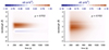 |
Fig. 2. Time evolution of Sun-as-a-star spectrum ΔS of Hα line with respect to wavelength and time for cases with Fpeak = 1 (left) and Fpeak = 10 (right) when flare occurs at the disk center (μ = 0.953). Red and blue represent enhancement and reduction, respectively. |
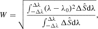
We now introduce three quantities that describe the properties of the line. The equivalent width ΔEW is calculated simply by integrating ΔS over wavelength. The integration range is ± 4 Å here in order to include the major variations in the profile. The line asymmetry A is obtained by the following equation:
 (6)
(6)
We followed Eq. (4) in Wu et al. (2022) and carried out an extra normalization. We set Δλ to be 0.5 Å. This quantity A(t) indicates red asymmetry for a positive value and blue asymmetry for a negative value. As for the line shift, we did not apply the two-component method (see Namekata et al. 2022a) since ΔS shows irregular profiles rather than double peaks. Here, we chose the bisector method, which is generally used on solar flares (Canfield et al. 1990), that is, finding a wavelength λm to make  , and here δλ is set to 1 Å. We chose to apply this method to
  rather than ΔS because the shape of
  is nearly symmetric after being averaged by the mainly quiet region of the disk. We can expect that the line shift values are quite small; thus, we primarily focused on the tendencies of these curves, which also contain useful information.
The result is shown in Fig. 3. For both weak and strong flares, the equivalent width increases rapidly and then decreases slowly, which follows the curve of the injected energy rate very well. The sign of the line shift and the line asymmetry depends on Fpeak: the weak flare presents a blueshift and red asymmetry, while the strong flare presents a redshift and blue asymmetry. After checking the other cases, we conclude that the line asymmetry of the Hα line always shows a negative correlation with the line shift.
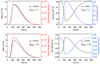 |
Fig. 3. Quantities as functions of time. Left: Injected energy rate of nonthermal electron beam (red line) and equivalent width (black line). Right: Line shift measured from bisector method (black line) and red asymmetry calculated from Eq. (6) (blue line). Positive values represent redshift and red asymmetry. |
Focusing on the evolution tendency of the three quantities above, the curve of ΔEW always follows that of the injected energy rate, but with a delay of tens of seconds. The curves of the line asymmetry and the line shift can have different behaviors. They might follow the energy rate curve as shown in the figure, and they might also deviate quite a lot as in cases Fpeak = 5 and 6 (see Fig. B.1). Thus, we consider the ΔEW of Hα as a good “real-time” indicator of the flare rather than the other two, regardless of flare locations (refer to Fig. B.2). From the perspective of line formation, the ΔEW depends highly on line enhancement and broadening. When the electron energy is released, and the line formation region is heated, the temperature there increases significantly, which immediately increases the ΔEW. However, the line asymmetry and the line shift result from the line-of-sight velocity of the plasma. Such a motion changes over simulation time (Kuridze et al. 2015; Hong et al. 2019) and is not directly related to the injected energy. It is worth mentioning that Namekata et al. (2022a) proposed the AIA 1600 Å curve as a proxy of the time profile of the energy release, which is somehow similar to the equivalent width.
As Fpeak increases, the blueshift as measured from the Sun-as-a-star spectrum changes to the redshift. To test whether the measured quantity reflects real motions in the atmosphere, we calculated the contribution function of t = 30 s of a single thread in both cases (see Fig. 4). The contribution function is defined as  , where jλ and τλ are the emissivity and optical depth, respectively. Integrating Cλ along the height, we obtain the emergent intensity. When Fpeak = 1, the line forms in the upper chromosphere (about 1.5 Mm). In this region, the plasma moves upward, which corresponds to the blueshift. As for case Fpeak = 10, the line forms lower and in a more concentrated way (about 1.3 Mm); the plasma moves downward and shows the redshift in our result. We checked the other eight cases and find that the plasma in the line formation region gradually shifts from upward movement to downward movement with increasing Fpeak, with the turning point at around Fpeak = 6. This accounts for the weakened blueshift signal as Fpeak increases. To account for the relationship between the line asymmetry and the line shift, we used the same interpretation as Kuridze et al. (2015): upward motion in the line formation region shifts the line core to the blue side, meaning more photons are absorbed in the blue wing. Consequently, the intensity in the red wing is larger compared to its blue wing counterpart, resulting in a red asymmetry. A similar explanation is used for redshift and blue asymmetry. The picture of Cλ shows that the bisector method is reasonable for detecting plasma motion in the chromosphere, at least for the velocity sign.
 |
Fig. 4. Line formation of Hα line at t = 30 s of single thread with Fpeak = 1 (left) and Fpeak = 10 (right). Lighter shades in the background denote larger values of the contribution function. The optical depth unity (red line) and the vertical velocity (blue line) as a function of height are overplotted, and the line profile is shown with a green line (right axis). |
3.2. Dependence on flare location
According to the Eddington-Barbier approximation – Iν(μ)≈Sν(τ = μ) – the emergent intensity of location μ depends on the source function where τ = μ. The line intensities at different locations reflect different layers of the solar atmosphere. Closer to the limb, μ is smaller; thus, we have properties in the shallower atmosphere, which causes the center-to-limb variation. In brief, the spectra show different profiles with respect to location, whether in quiet or flare regions.
Figure 5 presents the variation of ΔS at different locations when Fpeak = 1. Case μ = 0.047 is not shown, because the ΔS of such an event is too weak to be detected after being multiplied by μ (Eq. (4)). At each μ, the spectra show apparent red asymmetry and line broadening, which are similar to those found by Namekata et al. (2022a). From μ = 0.953 to 0.231, the maximum value of ΔS reduces because the projection area of the flare becomes smaller. We then focused on the profiles of ΔS when μ decreases. On one hand, the enhancement is more concentrated in the line core when μ = 0.953, but it has a larger spread when μ = 0.231. On the other hand, the profile shows multi-peaks, with most lying in the line wing instead of the line center. The absorption dip in the blue wing has negative values at the disk center, but it is less pronounced toward the solar limb. For strong flares (Fig. 6), the variations in different locations are similar to the weak ones, but with generally larger values of ΔS and a redshifted absorption dip.
 |
Fig. 5. Sun-as-a-star spectrum ΔS of Hα line of wavelength and time at different flare location μ when Fpeak = 1. The rest are the same as in Fig. 2. |
In order to focus more on profile shapes rather than values, we normalized ΔS by the maximum value of the whole profile at each time:  . Then, we plotted
  over different μ in cases Fpeak = 1 and 10 in Fig. 7. We show the result of t = 200 s, which is the peak time of our flare model. In the weak flare, values of
  at the red wings are larger than those at the blue wings, which is mainly caused by the blueshift, as discussed in Sect. 3.1. For the strong flare, the result is exactly the opposite: redshift decreases the values at the red wings and increases them at the blue wings.
 |
Fig. 7. Normalized profile |

As noted above, the width and dip of the normalized profile  vary with μ and Fpeak. For a quantitative analysis, we define the following two quantities to extract useful information from the profiles. One is the line width, defined as the second moment of the normalized profile
  ,
,
 (7)
(7)
where λ0 is the wavelength at the line center, and the value of Δλ is set to 4 Å.
We calculated the line width of both Hα and Hβ lines in different models and show the results in Fig. 8. The patterns in these two lines are quite similar. A larger Fpeak and a smaller μ would result in a larger W, which is also revealed from Fig. 7. The value of W(Hα) varies from 1.0 (the smallest Fpeak and the largest μ) to 2.3 (the largest Fpeak and the smallest μ), while the value of W(Hβ) is smaller, ranging from 0.4 to 1.5. We also note that the dependence on μ is more pronounced than that on Fpeak. For smaller values of μ, the line width does not vary much with Fpeak.
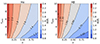 |
Fig. 8. Filled contours of line width W of Hα (left) and Hβ (right) line as a function of μ and Fpeak. |
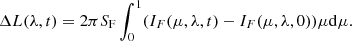
The other quantity is dΔS, which measures the relative difference between the line core and line wings:
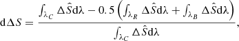 (8)
(8)
where λC, λR and λB are integration ranges for the line core, red wing, and blue wing. We chose λC = [−0.5 Å,0.5 Å], λR = [0.5 Å,1.5 Å] and λB = [−1.5 Å,0.5 Å] for the Hα line. For Hβ, the ranges of λC, λR, and λB are set to [−0.22 Å,0.22 Å], [0.22 Å,0.66 Å], and [−0.66 Å, −0.22 Å], respectively. A negative dΔS indicates a dip in the line core.
The results of dΔS are plotted in Fig. 9. For both lines, the value of dΔS has a weak dependence on Fpeak for 0.2 < μ < 0.4. The dependence on Fpeak becomes more pronounced when μ is larger than 0.6 or smaller than 0.2. For both W and dΔS, the dependence on μ is always strong regardless of the value of Fpeak. These two contours can be combined as diagnostics of the flare location from the observed line profiles, which are discussed further in Sect. 4.3.
4. Comparison with observations
4.1. Contrast profiles
Aside from the method mentioned in Sect. 2.3, the other approach to analyzing the Sun-as-a-star spectrum is to calculate the contrast profile (Pietrow et al. 2024a). The contrast profile R is obtained by normalizing  with the quiet spectrum:
  . When normalizing, the values of the quiet spectrum on the denominator vary over wavelength, rather than a constant as in Eq. (4), so shapes of R evidently differ from ΔS. We show R of four synthesized chromospheric lines (Hα, Hβ, Ca II K, and Ca II H) with respect to two parameters at t = 200 s in Fig. 10. The shapes of the Hα and Hβ contrast profiles look similar, which is also the case between the Ca II K and Ca II H profiles. However, the Hβ and Ca II K contrast profiles are wider and stronger than those of Hα and Ca II H, respectively. In these cases, the contrast profiles of Ca II are stronger and wider than that of H I, which indicates that Ca II lines are more sensitive to flares under nonthermal electron beam heating. As Fpeak increases and μ decreases, the triple-peak profiles of the Ca II lines become more pronounced.
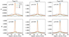 |
Fig. 10. Contrast profile R of Hα, Hβ, Ca II K, and Ca II H lines in different models. The parameter Fpeak varies among 1 (Left), 5 (middle), and 10 (right), while μ varies between 0.231 (top) and 0.953 (bottom). |
Compared to observations of the X-class flares in (Pietrow et al. 2024a), the intensity of R in our simulation is much smaller, even if for the strongest case (Fpeak = 10, μ = 0.953). The observed contrast profiles of each line (particularly Ca II lines) are also wider than simulations. One reason for these differences is that our flare area is not as large as those in their observations. We used the same flare area (1.5 × 1018cm2) to calculate the soft X-ray flux in our models following Pinto et al. (2015), assuming the radiation mechanism to be a thermal bremsstrahlung one. An optically thin assumption is also employed here, meaning that the X-ray flux is independent of μ. The corresponding GOES soft X-ray flux is partly shown in Fig. 11. We find that for different flares in our simulation, as the electron beam flux increases, the increase in soft X-ray flux is larger than the increase in the contrast profiles. This implies that in order to reach the same soft X-ray flux level, a larger flare area with a smaller beam flux would result in a larger value in the contrast profile. Pietrow et al. (2024a) also noted a red wing enhancement in Ca II K of the observed X9.3 flare implying chromospheric condensation (Malcolm Druett, private communication), while the red wing enhancement only appears in both weak and limb flares in our models (see the upper left panel of Fig. 11), and is the result of weak-upflowing absorptive plasma at the bottom of the evaporation region (see the left panel of Fig. 4).
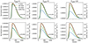 |
Fig. 11. Time evolution of S-index, Hα-index, and Hβ-index; arrangement order of parameters is similar to that in Fig. 10. |
4.2. Activity indices
Several activity indices of chromospheric lines have been defined to quantify the strength of stellar chromospheric activities (Boisse et al. 2009; Melbourne et al. 2020; Amazo-Gómez et al. 2023). In the quiet-Sun profiles, the line centers of these lines form in the chromosphere, while the line wings form in the photosphere. During flaring activities, especially when heating is dominated by a nonthermal beam, the upper chromosphere is heated more efficiently than the lower layers. Consequently, the line center that is formed in the chromosphere exhibits a stronger response than the wings and the continuum. This result holds even though flares can produce additional strong chromospheric sources in the line wings and bound-free continua (Allred et al. 2015; Simões et al. 2017; Druett & Zharkova 2018). Vaughan et al. (1978) introduced the concept of S-index, which is the ratio between the line core of Ca II H/K and the nearby continuum.
In quiet-Sun profiles, the line centers form in the chromosphere, while the line wings form in the photosphere. During flaring activities, especially when heating is dominated by a nonthermal beam, the upper chromosphere is heated more efficiently than the lower layers. Consequently, the line center that is formed in the chromosphere exhibits a stronger response than the wings and the continuum. We followed Melbourne et al. (2020) to calculate the S-index as
 (9)
(9)
where the line fluxes FH and FK are the integration of the astrophysical flux over the 1.09 Å wide triangular bands centered on 3933.66 Å and 3968.46 Å, and the near-continuum fluxes FR and FV are integrated over ±10 Å centered on 3901 Å and 4001 Å, respectively. The Hα-index is calculated as
 (10)
(10)
where FHα is the integrated flux over 0.6 Å around the Hα line center (6562.8 Å) and F1 and F2 correspond to the continuum flux integrated over 8 Å windows centered at 6550.85 and 6580.28 Å, respectively. Similarly, for Hβ, the index is obtained by setting the wavelength centers of the integration ranges of FHβ, F1, and F2 to 4861.38, 4585, and 4880 Å, with a window width of 0.2, 10, and 10 Å, respectively. Wavelength window values are the same as those of Pietrow et al. (2024a), who use relatively narrower windows in the line center to reduce the wash-out effect by the photosphere. Pietrow et al. (2024a) suggests that the Hα and Hβ index values are strongly dependent on the width of these windows, so here we only compare our results to their observations.
We plot the time evolution of the three indices in Fig. 11. The indices in the observation often exhibit much more noise compared to our simulation, which explains why only strong flares are detectable from the indices in the observations. Considering the X9.3 flare reported by Pietrow et al. (2024a), it results in an approximately 1% increase of the S-index and a 0.5% increase of the Hα/Hβ index. In our simulation, even for the strongest case (bottom right panel), we see an approximately 0.02% increase of the Hα/Hβ-index and a 0.01% increase of the S-index, which is nearly one fifth of that in Pietrow et al. (2024a). As discussed above, one possible reason is that the flare class is not large enough. Another reason is that the contrast profiles are narrower than those in Pietrow et al. (2024a). For case Fpeak = 10, μ = 0.953 (bottom right panel in Fig. 10), the double peaks of the Ca II K line wings are located at ±10 km/s, but at about ±70 km/s in the observation. The narrow profiles result in a much smaller increase of FH and FK, leading to a much smaller increase of the S-index. Considering the noise level in Pietrow et al. (2024a), it could still be difficult to detect the flare signal from the activity indices of our simulated X2 flare. Pietrow et al. (2024a) also reveals that the increase of the S-index has a longer duration compared to the other two indices. However, the longer duration of the S-index is not found in our simulation, since our simulation is only in one-dimensional, and we did not include the complexity of the multidimensional evolution and heating in solar flares (Druett et al. 2024; Ruan et al. 2024).
In solar flare observations, the soft X-ray flux of GOES 1–8 Å is also considered as an index to indicate flare magnitudes. We show the flux together with the three indices in Fig. 11. The GOES flux for the case of Fpeak = 1 is notably smaller due to the neglect of coronal heating by electrons below the cut-off energy. The peak of the soft X-ray curve has an approximately 30 s time delay compared to other index curves. Such a time delay is similar to those of observations reported in Namekata et al. (2022a), where the ΔEW of the Hα peaks faster than GOES X-ray. It seems that the heating of the chromosphere is faster than that of the corona in our model, which is a commonly observed relationship in solar flares and is one aspect of the relationship between the gradient of the soft X-ray flux curve and the hard X-ray flux curve known as the Neupert effect (Neupert 1968).
4.3. Diagnosing the flare location from observations
One of the primary objectives of our work is to find a method to diagnose the location of a stellar flare. In Sect. 3.2, we introduced two quantities – W and dΔS – and plotted their variations with respect to two parameters, μ and Fpeak. Both W and dΔS have a larger dependence on μ, and these contours can be used to locate the flare. For example, if dΔS(Hα) < 0, then μ should be less than 0.4 from Fig. 9, which makes it a near-limb event. By combining Figs. 8 and 9, one can determine the possible range of μ and Fpeak. Taking the Hβ line as an example, if W = 0.6 and dΔS = 0.4, we can diagnose that Fpeak is small and μ is large, meaning that a weak flare occurs near the disk center.
We point out that this diagnostic method only works well when the flare ribbon causes the majority of the variation of the Sun-as-a-star spectrum. In real observations, solar flares are sometimes accompanied by other transient phenomena such as surges, filament eruptions, and coronal rain. Usually, these events can be identified by their unique characteristics. For example, a sudden enhancement of ΔS shifting from the blue wing to the red wing may indicate an out-of-limb prominence eruption Otsu et al. (2022). An absorption of ΔS shifting from the blue wing to the red wing indicates a filament eruption or a surge on the solar disk (Ikuta & Shibata 2024). Nonetheless, as long as we exclude the interference events above, the characteristics of the spectrum can be systematically compared with our simulation. We take event 2 and event 4 of Otsu et al. (2022) as examples. The Sun-as-a-star spectrum of the limb flare (event 2) seems to appear as a central dip (see their Fig. 4), while that of the non-limb flare (event 4) shows a single-peak profile (see their Fig. 8), similarly to our results.
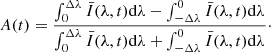
4.4. From flux to energy
As mentioned in Sect. 2, the astrophysical flux F (equivalent to  ) is measured in units of erg s−1 cm−2 sr−2 Å−1. In order to be compared with the Sun-as-a-star observation,
  must be converted into flux received by the detector (also known as the irradiance if the detector is on the Earth) as follows:
 (11)
(11)
with the solar radius R⊙ and distance D.
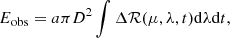
The next step is to determine the flare radiation energy from ℛ. As is known, a flare radiates energy in all directions. Since there is no “Dyson sphere”, it is impossible to detect the flux from a 4π solid angle. Therefore, in order to calculate the radiative energy, one should rely on some estimation methods. That is to say, one needs a conversion coefficient a between radiative energy E and irradiance ℛ:
 (12)
(12)
where Δℛ(μ, λ, t) = ℛ(μ, λ, t)−ℛ(μ, λ, 0). If the radiation is assumed to be isotropic, the coefficient a is then taken as four. This simple assumption has been employed in many previous works (Kowalski 2024; Notsu et al. 2024; Fletcher et al. 2011; Zhao et al. 2024). However, as discussed in Sect. 3, the flare spectra show significant differences if the flare occurs at different locations (e.g., the radiation enhancement at the disk center is greater than that at the disk limb). This indicates that flare radiation is not isotropic, making it inaccurate to choose four as the value of the coefficient. Woods et al. (2006) first considered such anisotropy. By integrating the limb darkening equation over the solid angle which is constrained by observations, they derived a coefficient of 1.4 for optically thick lines. For optically thin lines they assumed isotropy in the hemisphere, giving a coefficient of two. Kretzschmar et al. (2010) also adopted a = 1.4 in their calculations. However, in our simulation, we can directly calculate the energy due to flares without assumptions as the increase of the outward flux at the flare region surface:
 (13)
(13)
By integrating ΔL(λ, t) over wavelength and time, we may obtain the total radiated flare energy Esim:
 (14)
(14)
With both Esim (independent of the location) and ℛ (dependent of the location), we then calculate the coefficient a from Eq. (12) directly:
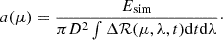 (15)
(15)
One should notice that the a is independent of D, R⊙, and SF. We show the results of a as a function of the location in Fig. 12.
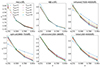 |
Fig. 12. Coefficient a in flux-energy conversion as a function of the flare location with different pass bands. Different colors indicate different flare magnitudes. |
We defined five pass bands: infrared (7500–40 000 Å), optical (3800–7500 Å), ultraviolet (200–3800 Å), Hα (6562.88 ± 5 Å), Hβ (4861.38 ± 3 Å), and total (200–40 000 Å). The majority of the solar irradiance lies in the wavelength range of 200–40 000 Å. The correlation of the coefficient a with μ for different Fpeak values is quite similar, although the results in weak flares have a large deviation. In each panel, a is negatively correlated with μ, which means that a near-limb flare requires a larger conversion coefficient from flux to energy than a disk-center flare. Except for two Balmer lines, the coefficient varies from about 1.6 to 2.3, with μ varying from 0.953 to 0.231. For the Hα and Hβ lines, the range of variation is greater; the coefficient at the center is 1.25 and can reach 3.0 at the limb, probably because the change in the chromosphere is more remarkable than in the photosphere. When the flare occurs at the disk center, the coefficient for the total pass band lies in the range of (1.58, 1.70), which is a little larger than the value of 1.4 in Woods et al. (2006). When μ equals 0.5, the coefficient is two, which is similar to that under the isotropic assumption in the hemisphere. The coefficient value range of different pass bands is listed in Appendix A for reference.
Such a variation is caused by two effects: the center-to-limb variation of the specific intensity and the projection effect. The former means that the enhancement of the specific intensity ΔIF varies with μ, while the latter requires ΔIF to be multiplied by μ (refer to Eq. (4)). If we only consider the projection effect, the coefficient is directly the reciprocal of μ, which becomes extremely large when μ is small. However, the coefficient does not significantly change with μ due to the compensation of the CLV of specific intensity: ΔIF at the limb is larger than at the center, meaning that limb flares are relatively brighter than center flares (see Fig. 4 and Sect. 3.3 in Cheng et al. 2010). This effect decreases the huge conversion coefficient caused by the small projection area of the limb flare, rendering a gentle change of a (compared to the 1/μ) in Fig. 12.
The flux-energy conversion relationship of a flare is significantly influenced by the flare location. For solar flares, since we can determine the location through imaging observations, it is easy to estimate the radiative energy in each pass band using the coefficient of Fig. 12. We can also determine the energy of a stellar flare if the flare location can be determined (refer to Sect. 4.3). However, the accuracy of a(μ) still needs to be confirmed by further observations with multiple pass bands.
4.5. Energy proportion of different pass bands
Stellar flare observations often give a light curve of a certain pass band. To estimate the total radiation energy of a stellar flare, the energy proportion of the pass band in the total wavelength is required. Here, we present the radiation energy proportion across different pass bands in Table 1. We note that the values are energy rather than flux, so they are independent of the flare location. The ratio of the optical, infrared, and ultraviolet radiation varies slowly with different Fpeak, but it is close to 3:2:5 for most cases. The contribution from the Balmer lines differs as the beam flux changes. For the Fpeak = 1 case, the Hα line contributes to less than 8% of the optical energy, but for the Fpeak = 10 case, the contribution drops to 2.6%. The ratio values in high beam-flux cases are similar to those in previous observations (1.8% in Namekata et al. 2022a and 1.5% in Namekata et al. 2022b), although they have used the assumption of black-body radiation for the optical continuum, which might underestimate the ratio to some extent (Simões et al. 2024). We notice that nearly one third of the flare energy comes from the optical pass band, with the majority attributed to the optical continuum. However, caution should be taken in categorizing these flares as observed “white-light flares” due to the instrumental sensitivity in real observations.
Energy partition of each pass band.
We also point out that the energy proportion is dependent on Ec and δ since different pass bands of photons arise from different depths of the atmosphere, and the beam penetration depth is strongly influenced by these parameters (Allred et al. 2015). It is also important that the beam parameters are believed to be highly dependent on location within the flare ribbon (Druett et al. 2017; Osborne & Fletcher 2022; Polito et al. 2023), as mentioned in Sect. 2.3. The relationship between energy proportion and flare properties remains to be confirmed.
5. Conclusion
In this paper, we present a Sun-as-a-star analysis of simulated solar flares. We begin by calculating the atmospheric response to nonthermal electron beam heating and the corresponding chromospheric lines in a single flare loop. Based on this single loop, we synthesize the Sun-as-a-star profiles using the multi-thread model. Two major parameters – electron beam flux Fpeak and flare location μ – are studied by analyzing the Sun-as-a-star spectra ΔS of the chromospheric lines. We summarize our results as follows.
-
The shape of ΔS(Hα) is characterized by the line enhancement and the line shift. Weak flares show apparent line shift, with an absorption at the blue wings. The line shift signal disappears when the flare occurs at the limb (see Fig. 5) or the flare energy is larger (see Fig. 2).
-
In weak flares, the Hα line shows a blueshift, resulting in a red asymmetry, while in strong flares it shows a redshift, leading to a blue asymmetry. The signs of line shift and line asymmetry are then always opposite. Compared to the line shift or the line asymmetry, the time evolution of the equivalent width of Hα is better correlated to that of the energy rate, making it a real-time indicator of the flare.
-
The profile of ΔS is highly dependent on the flare location. Getting closer to the disk limb, ΔS becomes wider and shows a more apparent dip in the line core, with multiple peaks at the wings. Two quantities – W and dΔS – are defined to measure the degree of the line width and the dip, respectively. For both Hα and Hβ lines, these two quantities have a stronger dependence on μ than Fpeak. Notably, when 0.2 < μ < 0.4, dΔS is primarily dependent on the location. We recommend using these two quantities to diagnose the location and magnitude of the stellar flare.
-
One needs a conversion coefficient a to calculate the radiation energy from the observed flux (Eq. (12)). We show that a is a function of the location μ. Additionally, the radiation energy proportion of different pass bands is presented in Table 1 for reference.
The above results in our simulations generally agree with previous observations. Yet, we will rely on more future observations, such as the full-disk observation of the Hα line by the Chinese Hα Solar Explorer (Li et al. 2019), to verify the models and diagnostics. On the other hand, simulations of other transient events including those by Yang et al. (2022) and Ikuta & Shibata (2024) are needed to distinguish these events from flares in the observations.
Acknowledgments
We thank the referee, Malcolm Druett, for his detailed and valuable suggestions that have greatly improved this paper. This project has been funded by National Key R&D Program of China under grant 2022YFF0503004 and by NSFC under grant 12127901. J.H. is also funded by the European Union through the European Research Council (ERC) under the Horizon Europe program (MAGHEAT, grant agreement 101088184). The Institute for Solar Physics is supported by a grant for research infrastructures of national importance from the Swedish Research Council (registration number 2021-00169).
References
- Allred, J. C., Kowalski, A. F., & Carlsson, M. 2015, ApJ, 809, 104 [NASA ADS] [CrossRef] [Google Scholar]
- Amazo-Gómez, E. M., Alvarado-Gómez, J. D., Poppenhäger, K., et al. 2023, MNRAS, 524, 5725 [CrossRef] [Google Scholar]
- Aschwanden, M. J., & Alexander, D. 2001, Sol. Phys., 204, 91 [NASA ADS] [CrossRef] [Google Scholar]
- Boisse, I., Moutou, C., Vidal-Madjar, A., et al. 2009, A&A, 495, 959 [NASA ADS] [CrossRef] [EDP Sciences] [Google Scholar]
- Canfield, R. C., Penn, M. J., Wulser, J.-P., & Kiplinger, A. L. 1990, ApJ, 363, 318 [NASA ADS] [CrossRef] [Google Scholar]
- Carlsson, M., & Stein, R. F. 1992, ApJ, 397, L59 [Google Scholar]
- Carlsson, M., & Stein, R. F. 1995, ApJ, 440, L29 [Google Scholar]
- Carlsson, M., & Stein, R. F. 1997, ApJ, 481, 500 [Google Scholar]
- Carlsson, M., & Stein, R. F. 2002, ApJ, 572, 626 [Google Scholar]
- Cheng, J. X., Ding, M. D., & Carlsson, M. 2010, ApJ, 711, 185 [NASA ADS] [CrossRef] [Google Scholar]
- Criscuoli, S., Marchenko, S., DeLand, M., Choudhary, D., & Kopp, G. 2023, ApJ, 951, 151 [NASA ADS] [CrossRef] [Google Scholar]
- Druett, M. K., & Zharkova, V. V. 2018, A&A, 610, A68 [NASA ADS] [CrossRef] [EDP Sciences] [Google Scholar]
- Druett, M., Scullion, E., Zharkova, V., et al. 2017, Nat. Commun., 8, 15905 [NASA ADS] [CrossRef] [Google Scholar]
- Druett, M., Ruan, W., & Keppens, R. 2024, A&A, 684, A171 [NASA ADS] [CrossRef] [EDP Sciences] [Google Scholar]
- Fletcher, L., Dennis, B. R., Hudson, H. S., et al. 2011, Space Sci. Rev., 159, 19 [Google Scholar]
- Haisch, B., Strong, K. T., & Rodono, M. 1991, ARA&A, 29, 275 [Google Scholar]
- Hong, J., Li, Y., Ding, M. D., & Carlsson, M. 2019, ApJ, 879, 128 [NASA ADS] [CrossRef] [Google Scholar]
- Hong, J., Carlsson, M., & Ding, M. D. 2022, A&A, 661, A77 [NASA ADS] [CrossRef] [EDP Sciences] [Google Scholar]
- Ikuta, K., & Shibata, K. 2024, ApJ, 963, 50 [NASA ADS] [CrossRef] [Google Scholar]
- Kerr, G. S., Carlsson, M., Allred, J. C., Young, P. R., & Daw, A. N. 2019, ApJ, 871, 23 [NASA ADS] [CrossRef] [Google Scholar]
- Kowalski, A. F. 2024, Liv. Rev. Sol. Phys., 21, 1 [NASA ADS] [CrossRef] [Google Scholar]
- Kowalski, A. F., Allred, J. C., Uitenbroek, H., et al. 2017, ApJ, 837, 125 [Google Scholar]
- Kretzschmar, M. 2011, A&A, 530, A84 [NASA ADS] [CrossRef] [EDP Sciences] [Google Scholar]
- Kretzschmar, M., de Wit, T. D., Schmutz, W., et al. 2010, Nat. Phys., 6, 690 [CrossRef] [Google Scholar]
- Kuridze, D., Mathioudakis, M., Simões, P. J. A., et al. 2015, ApJ, 813, 125 [Google Scholar]
- Li, Y., Ding, M. D., Hong, J., Li, H., & Gan, W. Q. 2019, ApJ, 879, 30 [NASA ADS] [CrossRef] [Google Scholar]
- Livingston, W., Wallace, L., White, O. R., & Giampapa, M. S. 2007, ApJ, 657, 1137 [CrossRef] [Google Scholar]
- Maehara, H., Shibayama, T., Notsu, S., et al. 2012, Nature, 485, 478 [NASA ADS] [Google Scholar]
- Melbourne, K., Youngblood, A., France, K., et al. 2020, AJ, 160, 269 [CrossRef] [Google Scholar]
- Namekata, K., Maehara, H., Honda, S., et al. 2021, Nat. Astron., 6, 241 [Google Scholar]
- Namekata, K., Ichimoto, K., Ishii, T. T., & Shibata, K. 2022a, ApJ, 933, 209 [NASA ADS] [CrossRef] [Google Scholar]
- Namekata, K., Maehara, H., Honda, S., et al. 2022b, ApJ, 926, L5 [CrossRef] [Google Scholar]
- Neupert, W. M. 1968, ApJ, 153, L59 [NASA ADS] [CrossRef] [Google Scholar]
- Notsu, Y., Shibayama, T., Maehara, H., et al. 2013, ApJ, 771, 127 [NASA ADS] [CrossRef] [Google Scholar]
- Notsu, Y., Kowalski, A. F., Maehara, H., et al. 2024, ApJ, 961, 189 [NASA ADS] [CrossRef] [Google Scholar]
- Osborne, C. M. J., & Fletcher, L. 2022, MNRAS, 516, 6066 [NASA ADS] [CrossRef] [Google Scholar]
- Otsu, T., & Asai, A. 2024, ApJ, 964, 75 [NASA ADS] [CrossRef] [Google Scholar]
- Otsu, T., Asai, A., Ichimoto, K., Ishii, T. T., & Namekata, K. 2022, ApJ, 939, 98 [NASA ADS] [CrossRef] [Google Scholar]
- Parker, E. N. 1963, ApJS, 8, 177 [NASA ADS] [CrossRef] [Google Scholar]
- Pereira, T. M. D., & Uitenbroek, H. 2015, A&A, 574, A3 [NASA ADS] [CrossRef] [EDP Sciences] [Google Scholar]
- Pietrow, A. G. M., & Pastor Yabar, A. 2024, IAU Symp., 365, 389 [NASA ADS] [Google Scholar]
- Pietrow, A. G. M., Hoppe, R., Bergemann, M., & Calvo, F. 2023, A&A, 672, L6 [NASA ADS] [CrossRef] [EDP Sciences] [Google Scholar]
- Pietrow, A. G. M., Cretignier, M., Druett, M. K., et al. 2024a, A&A, 682, A46 [NASA ADS] [CrossRef] [EDP Sciences] [Google Scholar]
- Pietrow, A. G. M., Druett, M. K., & Singh, V. 2024b, A&A, 685, A137 [NASA ADS] [CrossRef] [EDP Sciences] [Google Scholar]
- Pinto, R. F., Vilmer, N., & Brun, A. S. 2015, A&A, 576, A37 [NASA ADS] [CrossRef] [EDP Sciences] [Google Scholar]
- Polito, V., Kerr, G. S., Xu, Y., Sadykov, V. M., & Lorincik, J. 2023, ApJ, 944, 104 [NASA ADS] [CrossRef] [Google Scholar]
- Pulkkinen, T. 2007, Liv. Rev. Sol. Phys., 4, 1 [Google Scholar]
- Qiu, J., & Longcope, D. W. 2016, ApJ, 820, 14 [NASA ADS] [CrossRef] [Google Scholar]
- Ruan, W., Keppens, R., Yan, L., & Antolin, P. 2024, ApJ, 967, 82 [CrossRef] [Google Scholar]
- Rubio da Costa, F., Kleint, L., Petrosian, V., Liu, W., & Allred, J. C. 2016, ApJ, 827, 38 [NASA ADS] [CrossRef] [Google Scholar]
- Shibata, K., & Magara, T. 2011, Liv. Rev. Sol. Phys., 8, 6 [Google Scholar]
- Shibata, K., & Tanuma, S. 2001, Earth Planets Space, 53, 473 [NASA ADS] [CrossRef] [Google Scholar]
- Simões, P. J. A., Kerr, G. S., Fletcher, L., et al. 2017, A&A, 605, A125 [NASA ADS] [CrossRef] [EDP Sciences] [Google Scholar]
- Simões, P. J. A., Araújo, A., Válio, A., & Fletcher, L. 2024, MNRAS, 528, 2562 [CrossRef] [Google Scholar]
- Tsurutani, B. T., Gonzalez, W. D., Lakhina, G. S., & Alex, S. 2003, J. Geophys. Res.: Space Phys., 108, 1268 [CrossRef] [Google Scholar]
- Vaughan, A. H., Preston, G. W., & Wilson, O. C. 1978, PASP, 90, 267 [Google Scholar]
- Warren, H. P. 2006, ApJ, 637, 522 [NASA ADS] [CrossRef] [Google Scholar]
- Woods, T. N., Eparvier, F. G., Fontenla, J., et al. 2004, Geophys. Res. Lett., 31, L10802 [Google Scholar]
- Woods, T. N., Kopp, G., & Chamberlin, P. C. 2006, J. Geophys. Res.: Space Phys., 111, A10S14 [CrossRef] [Google Scholar]
- Wu, Y., Chen, H., Tian, H., et al. 2022, ApJ, 928, 180 [NASA ADS] [CrossRef] [Google Scholar]
- Xu, Y., Tian, H., Hou, Z., et al. 2022, ApJ, 931, 76 [NASA ADS] [CrossRef] [Google Scholar]
- Yang, Z., Tian, H., Bai, X., et al. 2022, ApJS, 260, 36 [NASA ADS] [CrossRef] [Google Scholar]
- Yu, H. C., Hong, J., & Ding, M. D. 2023, A&A, 675, A171 [NASA ADS] [CrossRef] [EDP Sciences] [Google Scholar]
- Zhao, Z. H., Hua, Z. Q., Cheng, X., Li, Z. Y., & Ding, M. D. 2024, ApJ, 961, 130 [NASA ADS] [CrossRef] [Google Scholar]
- Zhou, Y.-A., Hong, J., Li, Y., & Ding, M. D. 2022, ApJ, 926, 223 [NASA ADS] [CrossRef] [Google Scholar]
- Zills, G., Criscuoli, S., Bertello, L., & Pevtsov, A. 2024, Front. Astron. Space Sci., 10, 1328364 [NASA ADS] [CrossRef] [Google Scholar]
Appendix A: Additional table for Fig. 12
Values of conversion coefficient a.
Appendix B: Additional figures
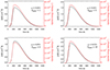 |
Fig. B.2. Injected energy rate of the non-thermal electron beam (red line) and equivalent width (black line) when flares occur at disk limb. |
All Tables
All Figures
|
Fig. 1. Occurrence rate P(t) (blue) and GOES 1–8 Å flux when Fpeak = 5 (red) as a function of time. The X-ray synthetic method is introduced in Sect. 4.1. |
| In the text | |
|
Fig. 2. Time evolution of Sun-as-a-star spectrum ΔS of Hα line with respect to wavelength and time for cases with Fpeak = 1 (left) and Fpeak = 10 (right) when flare occurs at the disk center (μ = 0.953). Red and blue represent enhancement and reduction, respectively. |
| In the text | |
|
Fig. 3. Quantities as functions of time. Left: Injected energy rate of nonthermal electron beam (red line) and equivalent width (black line). Right: Line shift measured from bisector method (black line) and red asymmetry calculated from Eq. (6) (blue line). Positive values represent redshift and red asymmetry. |
| In the text | |
|
Fig. 4. Line formation of Hα line at t = 30 s of single thread with Fpeak = 1 (left) and Fpeak = 10 (right). Lighter shades in the background denote larger values of the contribution function. The optical depth unity (red line) and the vertical velocity (blue line) as a function of height are overplotted, and the line profile is shown with a green line (right axis). |
| In the text | |
|
Fig. 5. Sun-as-a-star spectrum ΔS of Hα line of wavelength and time at different flare location μ when Fpeak = 1. The rest are the same as in Fig. 2. |
| In the text | |
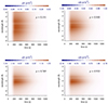 |
Fig. 6. Same as Fig. 5, but Fpeak = 10. |
| In the text | |
|
Fig. 7. Normalized profile |
| In the text | |
|
Fig. 8. Filled contours of line width W of Hα (left) and Hβ (right) line as a function of μ and Fpeak. |
| In the text | |
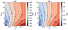 |
Fig. 9. Same as Fig. 8, but for dΔS. |
| In the text | |
|
Fig. 10. Contrast profile R of Hα, Hβ, Ca II K, and Ca II H lines in different models. The parameter Fpeak varies among 1 (Left), 5 (middle), and 10 (right), while μ varies between 0.231 (top) and 0.953 (bottom). |
| In the text | |
|
Fig. 11. Time evolution of S-index, Hα-index, and Hβ-index; arrangement order of parameters is similar to that in Fig. 10. |
| In the text | |
|
Fig. 12. Coefficient a in flux-energy conversion as a function of the flare location with different pass bands. Different colors indicate different flare magnitudes. |
| In the text | |
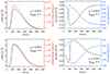 |
Fig. B.1. Same as Fig. 3 but Fpeak = 5 and 6. |
| In the text | |
|
Fig. B.2. Injected energy rate of the non-thermal electron beam (red line) and equivalent width (black line) when flares occur at disk limb. |
| In the text | |
Current usage metrics show cumulative count of Article Views (full-text article views including HTML views, PDF and ePub downloads, according to the available data) and Abstracts Views on Vision4Press platform.
Data correspond to usage on the plateform after 2015. The current usage metrics is available 48-96 hours after online publication and is updated daily on week days.
Initial download of the metrics may take a while.