| Issue |
A&A
Volume 694, February 2025
|
|
|---|---|---|
| Article Number | A314 | |
| Number of page(s) | 20 | |
| Section | Stellar structure and evolution | |
| DOI | https://doi.org/10.1051/0004-6361/202450514 | |
| Published online | 24 February 2025 | |
Seismic modelling of subgiant stars: Testing different grid interpolation methods
1
Instituto de Astrofísica e Ciências do Espaço, Universidade do Porto, CAUP, Rua das Estrelas, 4150-762 Porto, Portugal
2
Departamento de Física e Astronomia, Faculdade de Ciências da Universidade do Porto, Rua do Campo Alegre, s/n, 4169-007 Porto, Portugal
3
Université Côte d’Azur, Observatoire de la Côte d’Azur, CNRS, Laboratoire Lagrange, Nice, France
4
IRAP, Université de Toulouse, CNRS, CNES, UPS, 14 avenue Edouard Belin, 31400 Toulouse, France
5
LIRA, Observatoire de Paris, Université PSL, Sorbonne Université, Université Paris Cité, CY Cergy Paris Université, CNRS, 92190 Meudon, France
⋆ Corresponding author; This email address is being protected from spambots. You need JavaScript enabled to view it.
Received:
25
April
2024
Accepted:
19
December
2024
Abstract
Context. Grid-based modelling techniques have enabled the determination of stellar properties with great precision. The emergence of mixed modes during the subgiant phase, whose frequencies are characterised by a fast evolution with age, can potentially enable a precise determination of stellar properties, a key goal for future missions such as PLATO. However, current modelling techniques often consider grids that lack the resolution to properly account for the fast mode frequency evolution, consequently requiring the use of interpolation algorithms to cover the parameter space in between the grid models when applying model-data comparison methods.
Aims. We aim to reproduce the ℓ = 1 mode frequencies within the accuracy limits associated with the typical observational errors (∼0.1 μHz) through interpolation on a grid of subgiant models.
Methods. With that aim, we used variations of a two-step interpolation algorithm that considered linear and cubic splines interpolation methods and different age proxies (physical age, scaled age, and central density).
Results. The best results were obtained using an algorithm that considers cubic splines interpolation along tracks, linear interpolation across tracks, and central density ρc as the age proxy. This combination yielded, on average, an absolute error of 0.14 μHz but reached maximum absolute errors on the interpolated frequencies of 1.2 μHz for some models, which is an order of magnitude higher than the typical observational errors. Furthermore, we investigated the impact on the accuracy of the interpolation from changes in the physical properties of the stars, showing, in particular, how the addition of core overshoot can significantly affect the interpolation results.
Key words: asteroseismology / methods: statistical / stars: evolution / stars: fundamental parameters / stars: oscillations
© The Authors 2025
 Open Access article, published by EDP Sciences, under the terms of the Creative Commons Attribution License (https://creativecommons.org/licenses/by/4.0), which permits unrestricted use, distribution, and reproduction in any medium, provided the original work is properly cited.
This article is published in open access under the Subscribe to Open model. This email address is being protected from spambots. You need JavaScript enabled to view it. to support open access publication.
1. Introduction
As solar-type stars end their longest stage of evolution, by finishing the burning of hydrogen in their cores and leaving the main-sequence (MS) towards more evolved stages of evolution, their physical and chemical structure allow for the emergence of new interesting features. Supported by a combination of stellar pulsation theory and a tremendous amount of high-quality asteroseismic data from space missions such as the Convection, Rotation and planetary Transits mission (CoRoT; Baglin et al. 2006), Kepler (Gilliland et al. 2010; Koch et al. 2010), the Transiting Exoplanet Survey Satellite (TESS; Ricker et al. 2015; Campante et al. 2016; Cunha et al. 2019), and the upcoming PLAnetary Transits and Oscillations of stars mission (PLATO; Rauer et al. 2014; Cunha et al. 2021; Rauer et al. 2023; Goupil et al. 2024), these features can be used to make robust inferences on stellar properties, internal structure, and dynamics.
During the MS, turbulent motions drive global pulsation modes: the stochastic oscillations of solar-like pulsators. These are acoustic (or p-) modes and are maintained by the gradient of pressure fluctuation, being mostly sensitive to conditions in the outer part of the star. This is the case because their propagation cavities are located between the surface and an inner turning point (whose depth is strongly dependent on the mode degree ℓ). In addition, it is possible that MS solar-like stars also support internal gravity waves maintained by gravity acting on density fluctuations; internal gravity waves are essentially trapped beneath the convective envelope in a cavity that is mostly independent of the mode degree (Unno et al. 1989; Aerts et al. 2010; Cunha 2018). Nevertheless, despite some claims (Garcia et al. 2010; Fossat et al. 2017), it is not yet clear that these gravity (or g-) modes have been observed in the Sun.
The properties of p- and g- modes depend directly on the stellar structure, hence varying significantly with stellar mass and evolution. As a star evolves beyond the MS into the so-called subgiant phase, hydrogen fusion in a shell outside of the core supplies the star with energy as its core contracts and the buoyancy frequency increases significantly towards the centre. These structural changes cause the frequency of the g-modes to approach the frequency of the p-modes, resulting in the appearance of mixed modes. These modes are maintained by gravity acting on density perturbations in the deep interior and by the gradient of the pressure perturbation in the outer layers, both of which strongly constrain the interior structure of the star (Deheuvels & Michel 2011). They are also characterised by frequencies that have a fast evolution with age, which can potentially be used to determine stellar properties with great precision (Li et al. 2019).
Despite their potential, subgiant stars are not so well studied as MS stars and red giants since they are both less common than MS stars and fainter than red giants. However, major advances are expected, as subgiants constitute a significant fraction of the asteroseismic targets of TESS and of the upcoming PLATO mission.
Several fast, stable, and robust optimisation algorithms are now available to the community, such as AIMS (Asteroseismic Inference on a Massive Scale; Rendle et al. 2019), BASTA (BAyesian STellar Algorithm; Aguirre Børsen-Koch et al. 2022), SPInS (Stellar Parameters INferred Systematically; Lebreton & Reese 2020), and PARAM (Rodrigues et al. 2017). These algorithms provide a powerful diagnostic tool for the determination of stellar properties that allow for the determination of a representative set of models that best reproduce a given set of classical and asteroseismic constraints.
Most of the optimisation algorithms are grid based, requiring access to pre-computed grids of stellar models that span a given parameter space. This is quite different from a so-called on-the-fly modelling approach where the goodness of the fit is calculated while generating the stellar models. In this method, the set of models generated is of use only for the target being modelled, with the generation of a new set of models being required each time a new target is considered. This makes the on-the-fly modelling computationally expensive and less appropriate for a pipeline of an instrument observing a vast number of stars. However, there is also a drawback associated with the grid based method: When increasing the number of parameters of the models, the number of models on the stellar grid also increases, increasing the required storage and possibly decreasing the computational efficiency. Thus, expanding the grid to include more input parameters generally requires reducing the resolution of the initial grid, which in turn reduces the precision with which stellar properties are inferred. We note that despite their differences, these two modelling approaches are not necessarily mutually exclusive, as the result of grid searches may be used to restrict the region of parameter space being considered for the more refined model-on-the-fly analysis.
In order to guarantee a given precision on the inferred stellar properties needed (e.g. to ensure that the science requirements of a mission are satisfied), it may be required to couple a grid based approach with an interpolation algorithm. These algorithms are used to compensate for the lack of resolution in model grids by providing an approximate description of model predictions (e.g. the global and seismic properties) at points of the parameter space located in between the models of the initial pre-computed discrete grid.
Current optimisation codes, such as AIMS and BASTA, use (or may use) interpolation algorithms. Typically, the interpolation procedure considers a two-step process: (i) interpolation along the tracks, according to a chosen age proxy, and (ii) interpolation between evolutionary tracks, which amounts to interpolation in the parameter space defined by the grid parameters, excluding age.
Rendle et al. (2019) discuss the results of interpolation tests conducted while fitting observational data with AIMS. The authors compare their results with the typical uncertainties found in the literature for an MS target, 16 Cyg A, whose smallest and average uncertainties for ℓ = 0 modes are 0.04 and 0.08 μHz, respectively, and for a red giant branch (RGB) target, KIC 4448777, whose smallest and average uncertainties for ℓ = 0 modes are 0.014 and 0.018 μHz, respectively. For interpolation along evolutionary tracks, interpolation errors for ℓ = 0 modes were found to be smaller than both the smallest and average uncertainties from literature values, except for a small fraction of RGB tracks (less than 3% of the number of RGB tracks) characterised by low masses and high metallicities. For cross-track interpolation, their root mean square average errors are comparable to their literature reference value of 0.08 μHz.
For BASTA, Aguirre Børsen-Koch et al. (2022) only discuss the results of the complete interpolation procedure and restrict the analysis to MS stars. Using an interpolation procedure similar to that employed in AIMS, they show that the fractional differences in Δν between the original and the interpolated track are at the 10−4 level, which is an order of magnitude smaller than the relative uncertainty in Δν measured for the best Kepler targets. Li et al. (2020) test the interpolation of ℓ = 1,2 oscillation mode frequencies while investigating the dependencies of seismic stellar ages for 36 Kepler subgiants on helium fraction, the mixing-length parameter, and metallicity. Using cubic splines interpolation and physical age, τ, as the age proxy, the authors perform interpolation along a mass track with 1.20 M⊙, where models to be interpolated are separated by a time step of 6 × 10⁶ yr. For ℓ = 1 modes, the differences between interpolated frequencies and their true values were mostly below ∼0.05 μHz, especially for frequencies in the range of 0.5–1.5 νmax. Using the same method, interpolation of ℓ = 2 mode frequencies was found to work well for p-dominated modes but not for g-dominated ones. For 85% of the tested modes, frequency differences were found to be smaller than 0.2 μHz, but for the remaining poorly fitted g-dominated modes, differences can go up to 0.5 μHz.
In summary, among the literature works concerning grid based modelling of solar-like pulsators, only Li et al. (2020) performed interpolation tests on grids of subgiant stars. Yet, even in that case, the work focused exclusively on interpolation along evolutionary tracks. This highlights a lack of quantification of the accuracy of interpolation algorithms in the subgiant evolutionary phase.
In this work, we perform a characterisation of classical interpolation algorithms applied to the determination of the pulsation properties in the subgiant evolutionary phase and discuss the problems associated with them, establishing which method is capable of most accurately describing model frequencies interpolated both along and across evolutionary tracks of a two-parameter stellar grid. As a reference, we compare the interpolation errors with typical observational errors of δν∼0.1 μHz (Li et al. 2020), which we set as our accuracy aim.
In Section 2, we discuss what makes interpolation during the subgiant phase particularly challenging, further motivating our work. In Section 3, we describe the grid of stellar models and the classical interpolation methods we intend to characterise. In Section 4, we analyse the results and the interpolation errors associated with the application of the various interpolation methods to the stellar grid while considering different interpolation methods and age proxies. We start by considering only interpolation along an evolutionary track before addressing the more general case of interpolation across the mass tracks of the grid. We also discuss the influence that different grid resolutions have on the interpolation errors. In Section 5, we investigate the nature of a problem caused by interpolating mass tracks across the mass region where MS models start developing a convective core, discussing how the overshoot parameter fov influences the results. Finally, a summary of our main results is presented in Section 6.
2. The impact of subgiant mixed modes in interpolation
There have been numerous theoretical studies stating the potential of using the avoided crossings to accurately determining stellar ages during the subgiant phase, but none has fully considered their impact in grid interpolation. In this section, we motivate our work by discussing why some age proxies are more adequate than others when applying interpolation to typical grids of stellar subgiant models.
Along a given evolutionary track, p-mode oscillation frequencies change following the evolution of the mean density. In order to remove the impact of that evolutionary effect, we considered normalised frequencies defined by
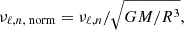 (1)
(1)
where G is the gravitational constant, M is the stellar mass, and R is the stellar radius of the corresponding model.
During the subgiant phase, we see the emergence of mixed modes whose frequencies exhibit a fast evolution, especially near the avoided crossings, that last about a couple tens of Myrs. For a fixed age, the same mode might be more acoustic- or gravity-dominated for different evolutionary tracks. This is shown in the top panel of Figure 1, which displays the evolution of the normalised frequency of a dipole mode of radial order n = 11 over various mass tracks, where we highlight a fixed value of age, of 4.18 Gyr, with a vertical dashed line. Because of this difference in the mode evolution at fixed age, when interpolating between different evolutionary tracks, we may be combining a mode that is evolving essentially as if it were acoustic (as in the case of the mass track with 1.23 M⊙), with a mode that is going through an avoided crossing (as in the case of the mass track with 1.24 M⊙). This difference in the mode evolution phase at fixed age is expected to impact the accuracy of the interpolation. One possible way to improve on that is to use proxies of age that better align the avoided crossings of adjacent mass tracks. One such proxy is the central density, ρc as illustrated in Figure 1. From the bottom panel, we see that avoided crossings appear more aligned when displayed as a function of the central density, ρc.
 |
Fig. 1. Evolution of the normalised frequencies of non-radial ℓ = 1 modes, with radial order n = 11, for evolutionary tracks of a stellar grid (the details of which are given in Section 3) with masses between 1.23 and 1.27 M⊙, as a function of the physical age τ (top) and the central density ρc (bottom). The points connected by a dashed line in the top panel indicate models with an age of 4.18 Gyr. The bottom panel displays a subplot that zooms on a particular avoided crossing for the mass M = 1.24 M⊙. |
To understand why ρc may be a better age proxy, we consider the evolution of the properties of the stellar core during the subgiant phase. When the H-burning ceases from being the main process of energy production in the core, the regions surrounding the isothermal He-core contract in order to increase pressure and temperature, triggering the H-burning process in a shell-boundary region around the core. This change in the structure influences the profile of the Brunt-Väisälä frequency in the stellar core. The increase in the Brunt-Väisälä frequency causes the frequency of g-modes to approach the frequency of p-modes, giving rise to a series of avoided crossings. In a fully ionised environment, the Brunt-Väisälä frequency can be written as
 (2)
(2)
where g is the local gravitational acceleration inside the star, HP is the local pressure scale height, ∇ad is the adiabatic gradient, ∇ is the temperature gradient, and ∇μ is the gradient of the mean molecular weight. Near the centre (r → 0), the local gravity inside the compact radiative subgiant core can be written as g(r)∼Gρcr. For an ideal gas in hydrostatic equilibrium, we thus find that the Brunt-Väisälä frequency scales as
 (3)
(3)
In early post-MS models, the central temperature, Tc, and the central mean molecular weight, μc, hardly change in the isothermal core where no nuclear reactions are happening. This leaves ρc as the main dependency of the Brunt-Väisälä frequency scaling in Equation (3). ρc increases monotonically during the subgiant phase due to the contraction of the inner regions of the star. It can, therefore, be considered as an age proxy for interpolation, with potential advantages compared to using physical age. In the following sections, we consider ρc and other age proxies to test grid interpolation accuracy during the subgiant phase.
3. Characterisation of the method
We start by describing the grid of stellar models used for our simulation tests and the procedure adopted to characterise the accuracy of linear and higher-order interpolation algorithms.
3.1. Input physics of the stellar grid
To perform tests that characterise the quality of interpolation, we compute a mass-age grid of evolutionary tracks in the subgiant phase. To this end, we used Modules for Experiments in Stellar Astrophysics (MESA, version r12778), an open-source stellar evolution package that is undergoing active development (Paxton et al. 2011, 2013, 2015, 2018, 2019). We adopted the solar composition from Asplund et al. (2009) and the OPAL opacity tables given by Grevesse & Sauval (1998), which were supplemented by the low-temperature opacities from Ferguson et al. (2005). We used the nuclear reactions rates obtained from the Joint Institute for Nuclear Astrophysics Reaction Library (JINA REACLIB, Cyburt et al. 2003) version 2.2, with specific rates for 12C(α, γ)16O (Kunz et al. 2002) and 14N(p, γ)15O (Imbriani et al. 2005). The boundary conditions at the stellar surface were established using the Krishna-Swamy atmosphere (Krishna Swamy 1966).
Our aim with this work is to test the interpolation across evolutionary tracks of different masses. Even though the ultimate goal is to test interpolation in a full grid where all parameters vary, we decided to keep things as simple as possible, by fixing all the physical inputs of the grid except for mass. Thus, we fixed metallicity at [Fe/H] = −0.1 dex, and varied the stellar mass between values of 1.150 and 1.350 M⊙, in steps of 0.005 M⊙. The goal was to produce a small but dense grid of stellar models in the subgiant phase, with masses crossing the region where small convective cores develop during the main sequence. The initial helium fraction was determined following the law of Galactic enrichment,
 (4)
(4)
where the primordial helium abundance is Y0 = 0.2485, according to Planck Collaboration XIII (2016), and the ratio ΔY/ΔZ is estimated to be 1.36 (Balser 2006; Nsamba et al. 2021). We also adopted the solar chemical mixture provided by Asplund et al. (2009), (Z/X)⊙ = 0.018099. The mixing-length parameter (first established in Böhm-Vitense 1958) is defined by αMLT = ℓMLT/HP, where ℓMLT is the mixing length, and HP is the pressure scale height. In MESA, αMLT is implemented by the mlt module for convection, as presented by Cox & Giuli (1968), and, for this grid, was fixed as 1.711. Convective overshooting was implemented via an exponential decay of the convective diffusion coefficient beyond the convective boundary, according to Herwig (2000),
 (5)
(5)
where Dconv,0 is the diffusion coefficient at the convective border, z is the distance from the boundary of the convective region, and fov is a user-adjusted dimensionless parameter set to 0.01. For small convective cores, MESA allows the implementation of convective overshoot through a geometrical cut-off (Paxton et al. 2011) that assures that overshoot is always limited to a fraction of the extension of the convective region. This is done by replacing HP in Equation (5) by
 (6)
(6)
where ΔRcz is the thickness of the convectively unstable region and αov is by default set to the mixing length parameter. Microscopic diffusion was not included.
The stellar models for all evolutionary tracks from the Hayashi line to the bottom of the red-giant branch were computed using MESA, but only the models from the subgiant phase were saved. This stage of evolution corresponds to the models calculated between the Terminal Age of the Main Sequence (TAMS), defined as when log(ρc)≃3.0 g.cm−3 (corresponding approximately to the age at which the central hydrogen abundance is Xc = 10−4 in our grid), and the Terminal Age of the SubGiant phase (TASG), defined as when log(ρc)≃4.5 g.cm−3 (Nsamba et al. 2018). Although unconventional, this ρc-condition for TAMS allows us to structure the grid with a constant ρc-step, starting from models with the same ρc value.
Computing a grid of stellar models capable of comprehensively describing oscillation modes in the subgiant phase is time-consuming as mixed modes vary rapidly with age. We programmed MESA to output models at a ρc-step of approximately 10 g.cm−3, which resulted in a dense grid of 121 424 stellar models distributed over the 41 evolutionary tracks, with the number of models per evolutionary track varying between 2959 and 2963. As the models of our stellar grid are equally spaced in central density, the number of models in the later stages of evolution is much larger than the number of models in the earlier stages of evolution, as seen in Figure 2, where we plot one in every 10 models along evolutionary tracks for illustration purposes. This information is important in order to correctly interpret the results we will present in our figures and tables.
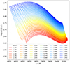 |
Fig. 2. Hertzsprung–Russell diagram displaying every tenth model of each of the 41 tracks in the subgiant phase produced for the stellar grid described in the text. |
For each model generated by MESA, we used GYRE (Townsend & Teitler 2013) to compute theoretical stellar oscillation frequencies for modes with ℓ = 0 and 1, by solving the equations for adiabatic stellar pulsations, outputting the frequencies within the frame window determined by
![Mathematical equation: $$ \begin{aligned}{[\nu _{\ell ,n}]} = \nu _{\rm max} \pm 3\sigma _\nu \text{,} \text{ where} \sigma _\nu = \frac{0.66 \nu _{\rm max}^{0.88}}{2\sqrt{2\log (2)}}, \end{aligned} $$](/articles/aa/full_html/2025/02/aa50514-24/aa50514-24-eq7.gif) (7)
(7)
where νmax is the frequency of maximum power, and σν is the width of the Gaussian envelope encompassing the distribution of pulsations, as given by Mosser et al. (2012).
While all radial orders of ℓ = 0 modes determined by GYRE within the frame window defined by Equation (7) were considered, only positive radial orders of ℓ = 1 modes were used in the tests. Only non-radial modes of degree ℓ = 1 were computed since the objective is to compare the interpolation of pure acoustic modes (ℓ = 0) with the interpolation of mixed modes (of which ℓ = 1 modes are the best example, since their p–g coupling is maximal).
3.2. Interpolation methods
A complete interpolation process requires both interpolation along the evolutionary track (i.e. in the age proxy), and across the input parameters of the grid (in this case, mass). Therefore, we considered a series of interpolation methods to explore the regions between stellar models, dividing the procedure in two steps: (i) age interpolation between models within an evolutionary track, considering a certain age proxy, and (ii) track interpolation across different evolutionary tracks (in the mass parameter), for a constant value of the previously chosen age proxy.
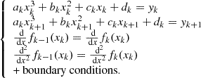
For the interpolation procedure, we considered first (linear) and third (cubic) order methods, contemplating either polynomial or spline interpolation. Polynomial interpolation usually fits a n order function to n + 1 points, and is used to interpolate between the middle two. Spline interpolation considers a set of n order functions, each defined between two data points to build a system of equations, constrained so that the values of the function and of its first and second derivatives match as one approaches each data point from the left and right. These requirements still leave the system under-constrained, which requires some reasonable assumptions to be made about the values beyond the range of data being fitted, usually an assumption about the 2nd derivative at the two end points. In both cases, the interpolated functions pass through all the existing points of the initial stellar grid. For example, consider an evolutionary track of a given mass M and a mode of a given radial order n (or similarly, consider a fixed value for a given age proxy τ and a mode of a given radial order n). Between every two models (x1, x2) on that evolutionary track (or at a fixed age proxy), we can linearly interpolate the frequencies to any point x within that interval by computing
 (8)
(8)
where y1 and y2 are the mode frequencies of radial order n in the models x1 and x2, respectively.
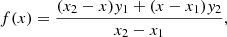
In the case of cubic splines, interpolation is accomplished using the function
![Mathematical equation: $$ \begin{aligned} f(x)= {\left\{ \begin{array}{ll} a_1x^3+b_1x^2+c_1x+d_1,\ \text{ if}\ x\in [x_1,x_2]\\ a_2x^3+b_2x^2+c_2x+d_2,\ \text{ if}\ x\in ]x_2,x_3]\\ \ldots \\ a_kx^3+b_kx^2+c_kx+d_k,\ \text{ if}\ x\in ]x_k,x_{k+1}] \end{array}\right.}, \end{aligned} $$](/articles/aa/full_html/2025/02/aa50514-24/aa50514-24-eq9.gif) (9)
(9)
where each of the four coefficients (ak, bk, ck, dk) that define a segment ]xk, xk + 1] of the resulting function is obtained by solving the system of equations
 (10)
(10)
We note that each polynomial from Equation (9) is valid within the respective intervals only. For interpolation in Python, we used the library package scipy.interpolate.interp1d(), while considering its default conditions. This includes boundary conditions established by a ‘not-a-knot’ condition, that is the first two polynomials’ third derivatives are equal in the point where they touch each other.
For each choice of the interpolation method, we can consider different age proxies for interpolation. Here we consider three options, namely, physical age, τ; scaled age, τscaled; and central density, ρc, with
 (11)
(11)
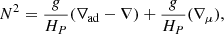
For each model i, the errors associated with each interpolation method and chosen age proxy are given by
 (12)
(12)
where ‘theoretical’ and ‘interpolation’ stand for the value outputted by GYRE and by the interpolation algorithm considered, respectively. Dimensional versions of these errors were computed using the equation
 (13)
(13)
4. Characterisation of the interpolation errors
To characterise the interpolation errors, we define two metrics, namely: (1) the maximum error for a given mode degree ℓ (mℓ), i.e. the maximum absolute interpolation error observed for all modes in all interpolated models on the evolutionary track, and (2) the average offset of the mode degree ℓ (μℓ), calculated as a weighted mean of all absolute interpolated errors, |δνi, ℓ, n|, for all modes on all interpolated models on the evolutionary track. Specifically,
 (14)
(14)
where
 (15)
(15)
where the sum in n is over all the radial orders considered for an evolutionary track (cf. Section 3.1), while the sum in i is over all the models for a given radial order and evolutionary track. The weight wi, n ensures that the same weight is given to similar intervals of τscaled. This is to avoid that our metric is biased towards the evolved subgiants due to our grid having models similarly distributed in ρc, rather than in τscaled. In the sections that follow, we drop the index ℓ in the quantities mℓ and μℓ and the index i in δνi, ℓ, n.
4.1. Interpolation along evolutionary tracks
We started by performing a control study of the errors on the frequencies that result from applying interpolation along an evolutionary track. Accordingly, we consider all evolution frequency curves (each defined by a different fixed radial order) determined for the mass track with M = 1.245 M⊙, and contemplate two possible interpolation methods – linear interpolation and cubic splines, – and three possible age proxies – τ, τscaled and ρc. The results are displayed in Figure 3 and Table 1 for ℓ = 0, and in Figure 4 and Table 2 for ℓ = 1, according to their maximum errors, m, and average offsets, μ, defined above.
 |
Fig. 3. Interpolation errors presented as a function of τscaled (bottom x-axis) and ρc (top x-axis) that resulted from interpolation along the evolutionary track with M = 1.245 M⊙ for all ℓ = 0 frequency modes, with radial orders n ∈ [9, 23] indicated by different colours. Each subplot presents the results for a different interpolation method, considering different methods – linear (top panels) or cubic splines (bottom panels) – and different age proxies – τscaled (left) and ρc (right). |
Average offsets (μ) and maximum errors (m) for different age proxies.
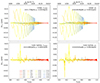 |
Fig. 4. Interpolation errors presented as a function of τscaled (bottom x-axis) and ρc (top x-axis) that resulted from interpolation along the evolutionary track with M = 1.245 M⊙ for all ℓ = 1 frequency modes, with radial orders n ∈ [1, 20] indicated by different colours. Each subplot presents the results for a different interpolation method, namely linear (top panels) and cubic splines (bottom panels), and different age proxies – τscaled (left) and ρc (right). |
Average offsets (μ) and maximum errors (m) for different age proxies.
The results of interpolation along evolutionary tracks considering τ as the age proxy are exactly the same as when considering τscaled as the age proxy, since both age proxies are related by a proportionality constant (cf. Equation (11)) that does not vary within a fixed evolutionary track.
For radial modes, the average offset of the interpolation errors is about 3 orders of magnitude smaller than the accuracy limit we set (∼0.1 μHz). This is to be expected, since the frequencies of radial modes evolve smoothly and thus do not produce significant interpolation errors. We observe only a slight improvement when increasing the order of the interpolation (from linear to cubic splines) and do not observe a significant dependence on the adopted age proxy.
For the ℓ = 1 modes, we again observe that the interpolation errors are essentially independent of the age proxy considered. However, the results for the dipole modes show a significant dependence on the interpolation method, with the average offset resulting from linear interpolation being ∼19.8 times larger than the average offset obtained using cubic splines. This shows that the cubic splines interpolation method is preferred for interpolation along evolutionary tracks for dipole modes. Moreover, the results show that the maximum error when interpolating with cubic splines along the evolutionary track is about an order of magnitude smaller than the typical observational errors (∼0.1 μHz), leaving room for additional errors that will result from the interpolation across different evolutionary tracks, and that we will address in Sections 4.2-4.5.
We also emphasise that the results for the mass track considered for these tests, with M = 1.245 M⊙, are of similar magnitude to those obtained for other mass tracks, making this evolutionary track a good representative for interpolation along tracks.
4.2. Full Interpolation with τ and τscaled as age proxies
In this section, we consider the errors resulting from the application of the full interpolation algorithm employed in the computation of the frequencies of models that do not lie on a particular evolutionary track. To that end, we consider a subset of our grid composed only of the models whose third decimal place of the associated mass value is 0 (e.g. 1.240) in order to retrieve through interpolation the models of the initial complete grid (namely those whose third decimal place of the associated mass value is 5, as 1.245).
As before, the initial tests are performed for models with M = 1.245 M⊙, whose frequencies are computed through interpolation, and subsequently compared with the true frequencies computed in the initial grid with GYRE. These tests will then be extended to the full grid in Section 4.4 and in Appendix A. The interpolation is made using the corresponding adjacent evolutionary tracks from the subset grid (2 for linear interpolation across tracks and 4 for the cubic splines interpolation across tracks). The results considering cubic splines along an evolutionary track and linear interpolation across evolutionary tracks are shown in Figure 5 and Table 3 for ℓ = 0, and in Figure 6 and Table 4 for ℓ = 1. Results from interpolating ℓ = 1 modes using cubic splines both along and across evolutionary tracks are shown in Figure 7. In all three figures, the results from considering τ as the age proxy are shown on the top panels, and the results from considering τscaled as the age proxy are shown in the middle panels.
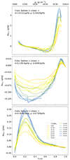 |
Fig. 5. Interpolation errors presented as a function of τscaled (bottom x-axis) and ρc (top x-axis) that resulted from the full interpolation algorithm (cubic splines interpolation along tracks, and linear interpolation across tracks) for all ℓ = 0 modes associated with the mass track M = 1.245 M⊙ when considering τ (top), τscaled (middle) and ρc (bottom) as the age proxies for interpolation. |
Average offset (μ) and maximum errors (m) for different age proxies.
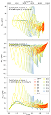 |
Fig. 6. Interpolation errors presented as a function of τscaled (bottom x-axis) and ρc (top x-axis) that resulted from the full interpolation algorithm (cubic splines interpolation along tracks, and linear interpolation across tracks) for all ℓ = 1 modes associated with the track with M = 1.245 M⊙ when considering τ (top), τscaled (middle) and ρc (bottom) as the age proxies for interpolation. |
Average offset (μ) and maximum errors (m) for different age proxies.
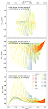 |
Fig. 7. Interpolation errors presented as a function of τscaled (bottom x-axis) and ρc (top x-axis) that resulted from the full interpolation algorithm (cubic splines interpolation both along and across tracks) for all ℓ = 1 modes associated with the track with M = 1.245 M⊙ when considering τ (top), τscaled (middle) and ρc (bottom) as the age proxies for interpolation. |
For radial modes (Figure 5), the best maximum errors and average offsets were obtained when τscaled is considered as the age proxy, with values of 1.4 × 10⁻¹ and 6.9 × 10⁻² μHz, respectively. This shows that, even for radial modes, interpolation errors can be larger than our goal, although not significantly so. Despite the absence of the avoided crossing phenomena, the evolutions of ℓ = 0 mode frequencies for different mass tracks are not aligned when described as a function of the age proxies considered. Thus, interpolation between different evolutionary tracks will still happen between different phases of evolution of the modes, as shown in Figure 8. This is more evident for the frequency evolution in age (top panel) than for the frequency evolution in τscaled (bottom panel), which is consistent with the errors presented in Table 3.
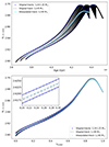 |
Fig. 8. Evolution of the scaled frequencies for the ℓ = 0 modes, with radial order n = 11, that resulted from applying the interpolation algorithm to the mass track with M = 1.245 M⊙, presented as a function of τ (top) and τscaled (bottom), when each is considered as the respective age proxy for interpolation. The bottom panel displays a subplot that zooms on the region of the age proxy parameter space with the highest interpolation errors. |
In the case of ℓ = 1 modes, the linear interpolation across tracks is again found to give better results when τscaled is taken as the age proxy (middle panel of Figure 6), this compared to using τ (top panel of Figure 6). However, the average offset of 5.6 × 10⁻¹ μHz and the maximum error of 3.6 × 100 μHz are already larger than our accuracy limit, with m being an order of magnitude larger than that limit. The reason for these errors when considering τ or τscaled as age proxy has been alluded to in Section 2 and can be further understood from the left and middle panels of Figure 9: because the mixed modes are not aligned when the frequency curves are described as a function of these age proxies, interpolation between different evolutionary tracks happens between different phases of evolution of the mixed modes, failing even when considering a relatively dense grid of models. Thus, for the cases presented, it is not possible to obtain results within the accuracy limit set by the typical observational errors, with this choice of methods and age proxies, which could potentially limit the use of stellar grids with interpolation to explore the parameter space when fitting seismic data for subgiant stars.
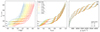 |
Fig. 9. Evolution of the normalised frequencies of non-radial ℓ = 1 modes with radial orders n = [10, 11, 12] for evolutionary tracks of the stellar grid with masses between 1.23 and 1.26 M⊙ as a function of the various age proxies considered for interpolation: τ (left), τscaled (middle), and ρc (right). Different colours are used to represent different stellar masses and different line styles show different radial orders, according to the insets in the middle and right panel, respectively. |
4.3. The central density ρc as an alternative age proxy
As discussed in Section 2, the avoided crossings of evolutionary tracks with different masses appear more aligned when displayed as a function of the central density, ρc (right plot of Figure 9). With the avoided crossings showing an increased alignment when described as a function of ρc, interpolation can happen between models whose mode frequencies are in a more similar phase of evolution, which is expected to lead to more accurate results.
With the above in mind, we now analyse the results from applying the full interpolation algorithm to interpolate the frequencies of models of the evolutionary track of M = 1.245 M⊙, using ρc as the age proxy. These results are shown in the bottom panels of Figures 5, 6 and 7, and summarised in Tables 3 and 4, for mode frequencies with ℓ = 0 and 1, respectively.
For the radial modes (ℓ = 0) (bottom panel of Figure 5), interpolation errors using ρc as the age proxy can be as high as 3.0 × 10⁻¹ μHz, only decreasing below 5.0 × 10⁻² μHz in later stages of evolution. In fact, this maximum error is close but slightly larger than the one obtained considering τscaled as the age proxy (m = 1.4 × 10⁻¹ μHz) and than the reference value of 0.1 μHz. This is not surprising since radial modes do not have avoided crossings; thus no particular improvement was to be expected by choosing ρc over τscaled as the age proxy. Although some of the radial orders produce interpolation errors above the established accuracy limit, these are limited to the models of the early subgiant phase with τscaled< 0.4. Despite these large maximum absolute errors in some models, the average offset is 7.3 × 10⁻² μHz, well within the proposed accuracy limit.
For ℓ = 1 modes, errors from interpolation considering ρc as the age proxy can be as high as 1.2 × 100 and 1.3 × 100 μHz, depending on the order of the interpolation method considered (Figures 6 and 7, respectively), only decreasing to values below 4.0 × 10⁻¹ μHz in the later stages of the subgiant evolution. Although their maxima are quite large (about an order of magnitude above the accuracy limit we set as reference), the average offset is improved by a factor of ∼3.9 over the average offset of interpolation with τscaled as the age proxy, yielding results similar to the expected accuracy limits – 1.4 × 10⁻¹ and 1.5 × 10⁻¹ μHz for linear and cubic splines interpolation, respectively. We verified that this improvement in the interpolation errors is not a consequence of the grid being equally spaced in ρc, rather than τscaled, (notice that the errors from interpolation along the tracks are always small, regardless of the age proxy being adopted when compared with the final errors (cf. Table 2)).
4.4. Results for the full grid
Next, we apply the analysis to the full grid and discuss the complete set of results. To this end, we use the mode frequencies determined as part of the subset (whose third decimal place of the associated mass value is 0) to obtain the frequencies for the missing mass tracks that also appear in the initial grid (i.e. those whose third decimal place of the associated mass value is 5). Results are presented in the tables in Appendix A, and summarised in Figure 10. Interpolation was not performed for tracks with masses 1.155 and 1.345 M⊙, given that they are near the limit where there are not enough models on one of the sides to allow cubic spline interpolation.
The results from Figure 10 show that using ρc as the age proxy significantly improves the accuracy of the interpolation when compared to τscaled. For M > 1.20 M⊙, both the average offset and maximum error are smaller when ρc is used, instead of τscaled, as the age proxy. For the smaller masses, there are a few cases when the interpolation errors obtained with the two age proxies are comparable, but only for one mass track both the average offset and the maximum error are larger when ρc is chosen. Moreover, we see that, with the exception of the mass track M = 1.175 M⊙ (brown dashed line in Figure 10), the average offset when taking ρc as the age proxy is always approximately within twice of the reference value. It also becomes evident that for the more massive evolutionary tracks the average offset when considering τscaled as the age proxy is similar to the maximum error found when ρc is chosen. Thus, when considering the full grid, the adoption of ρc in place of τscaled as the age proxy seems well justified. Finally, Figure 10 confirms that the evolutionary track of M = 1.245 M⊙ (brown dotted line), considered in the previous sections, has typical interpolation errors, justifying its use in the more detailed analysis presented, and it also shows that there is an evolutionary track (M = 1.175 M⊙) for which interpolation performs significantly worse. We shall address the origin of the anomalous large interpolation errors found for the latter model in Section 5.
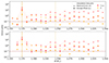 |
Fig. 10. Average offsets (μ, indicated by squares; in μHz) and maximum errors (m, indicated by triangles; in μHz) from the full interpolation method, which considers cubic splines along evolutionary tracks and linear (top) or cubic splines (bottom) interpolation across evolutionary tracks and τscaled (red) or ρc (yellow) as the age proxy, for all ℓ = 1 modes obtained for the interpolated tracks of the initial grid. The vertical brown dotted line highlights the results for our reference track with M = 1.245 M⊙, while the vertical brown dashed line highlights the anomalous track with M = 1.175 M⊙. |
4.5. Impact of the order of interpolation
Having discussed the results of interpolation considering different age proxies, we now compare the performance of the different orders of the interpolation when interpolating across evolutionary tracks, for a fixed value of the age proxy. We compare the results of applying linear interpolation (Figure 6) and cubic splines interpolation (Figure 7) to the ℓ = 1 modes of models in the mass track with M = 1.245 M⊙. These results (summarised in Table 4) show that the average offset and the maximum error hardly change when changing the order of the interpolation. This is true both when adopting τscaled and ρc as age proxies.
Considering that the full grid does not change these conclusions in any significant way, taking ρc as the age proxy, we found eight interpolated mass tracks for which linear interpolation performed better (i.e. resulting in smaller μ and m values than when employing the cubic splines), nine cases where cubic splines interpolation performed better, and one where the results were mixed (i.e. for M = 1.225 M⊙, the smallest μ and m values were not found using the same method). These results seem to indicate no clear preference for one of the interpolation methods when performing interpolation across evolutionary tracks. Moreover, inspection of the tables in Appendix A shows that the average offsets computed with linear and cubic splines interpolation on each individual track are almost always of the same order of magnitude. The most significant differences are found for M = 1.165 and 1.185 M⊙, for which μ from linear interpolation can be ∼6.18 and ∼3.19 times smaller than μ from cubic splines, respectively. These two cases, together with the mass track with M = 1.175 M⊙, which presents the highest interpolation errors of this grid (see Figure 10), span the region of the mass parameter space where the core properties of the modelled stars change and it shall be discuss in detail in Section 5.
Given the results presented in the previous subsections, we favour the interpolation option that considers the simplest approach and least computational expensive: cubic splines to interpolate along tracks, linear interpolation to interpolate across tracks, and ρc as the age proxy.
4.6. Testing the grid resolution
We now recall that every evolutionary track in the initial grid has between 2959 and 2963 models, with about half of them (∼1482 models) being used to determine the other half through interpolation. This is a large number of models occupying the memory of the system, and therefore, in what follows we assess the impact of the grid resolution on the interpolation errors. Considering the results from the previous sections, we divide this exercise in two parts, with two different objectives. The first concerns interpolation along evolutionary tracks, where we will verify what is the minimum number of models per track for which the results remain accurate within the accuracy limit.
With that objective in mind, we consider a number of subgrids, each with a fraction of the resolution of the initial grid, 1/k, where each evolutionary track is built by collecting every kth model of the initial track. In this study, we focus on the evolutionary track with M = 1.245 M⊙, and test grid resolutions between 1/1 (the initial grid) and 1/6 of the initial grid (which only contains ∼247 models per track for interpolation). Although we still test different interpolation methods, we establish ρc as a definitive age proxy. The results are summarised in Table 51.
Average offsets (μ) and maximum errors (m) for different grid resolutions.
We observe that both μ and m increase by a significant factor whenever the grid resolution is reduced. For a grid resolution of 1/6 of the initial grid, both the average offset μ and the maximum error m increase by more than 2 orders of magnitude. However, while the average offset μ changes from 3.4 × 10⁻⁴ to 1.3 × 10⁻¹ μHz, a value still close to the established accuracy limit, the maximum errors increase from 3.3 × 10⁻² to 3.4 × 100 μHz, this second value being significantly out of the established accuracy limit. In the initial grid, to keep the errors of the interpolation along evolution within values comparable to the goal, our results indicate that the minimal grid resolution recommended should be no less than 1/3 of the initial grid (i.e. a grid of stellar models containing ∼494 models per track for interpolation). In this case, the maximum error of 2.1 × 10⁻¹ μHz is only slightly higher than the established accuracy limit.
The second part of the exercise concerns the impact of the grid resolution on the interpolation across evolutionary tracks. In Section 4.4, we have found that the results for the current grid fail to comply with the reference accuracy in what concerns the maximum error, while performing reasonably close to the goal (within a factor of two) in what concerns the average offset, when ρc is used as the age proxy. Depending on the quality of the data, the accuracy achieved with our reference grid may therefore still suffice; in which case it is still interesting to understand whether a similar accuracy may be achieved with a reduced number of models. To test this, we repeat the exercise of decreasing the grid resolution for the case of full interpolation to understand the consequent impact on the interpolation errors.
Table 6 displays the results of the full interpolation algorithm applied to different grid resolutions, considering cubic splines for interpolation along, and either linear or cubic splines for the interpolation across. For the case we previously established as the preferred option (cubic splines along and linear across), we observe a smaller relative evolution of the interpolation errors with the resolution of the subgrid than when considering interpolation along evolution alone. Indeed, the average offsets remain close to the limit of accuracy, increasing only slightly until the subgrid with 1/6 of the models is considered. Moreover, the maximum errors, which are found to be out of the accuracy limit already in the initial grid, hardly change when the number of models is decreased to 1/3 of the initial value. The impact of decreasing it further, to 1/6 of the initial number of models, seems to depend on the order of the method applied for the interpolation across evolutionary tracks, with the option of cubic splines performing somewhat better when the number of models is significantly decreased.
Average offsets (μ) and maximum errors (m) for different grid resolutions.
In conclusion, we find that decreasing the number of models considered in each evolutionary track to ∼1/3 of the initial value does not impact the accuracy of the interpolation results from our grid in any significant way. However, we emphasise that, in all cases, the maximum interpolation errors found are significantly above the goal (as seen in Figure 10, and discussed in Section 4.4).
5. Influence of core properties on interpolation
In Sections 4.4 and 4.5, we noted that all measurements of the interpolation errors are significantly larger for the evolutionary track with M = 1.175 M⊙ (brown dashed line in Figure 10). Here, we investigate this case further, to understand the origin of the larger errors and the implications that this extreme case may have in the construction of future model grids. To further characterise this anomaly, we address the results from the perspective of a fixed radial order and multiple evolutionary tracks, corresponding to the different masses in the grid. To that end, we compute the average offset in a way similar to that presented in Equation (14), but with the average over radial orders replaced by an average over masses for the chosen radial order. Figure 11 presents the frequency interpolation errors for dipolar modes of radial order 11 as a function of the age proxies τscaled and ρc. For the mass track with M = 1.175 M⊙, the interpolation errors are not only about one order of magnitude larger than the typical errors found for the other masses, but they are also systematic, being always positive and always significant along the full evolutionary track. This problem is not restricted to one particular dipole mode. In fact, all modes associated with the mass track with M = 1.175 M⊙ present similar maximum errors, that can be as high as 7.7 × 100 μHz, and average offsets of the order of 1.7 × 100 μHz. This can be illustrated by focusing on a specific evolution point (e.g. at fixed ρc) and looking at how the interpolation error for a given radial order varies with mass. This is illustrated in Figure 12, where we find a discontinuity between the evolutionary tracks with M = 1.175 and 1.180 M⊙.
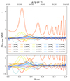 |
Fig. 11. Interpolation errors presented as a function of τscaled (bottom x-axis) and ρc (top x-axis) that resulted from the application of the full interpolation algorithm (cubic splines along tracks and linear across tracks) across the complete grid. Results are shown for all ν1, 11 mode frequencies, when ρc is considered as the age proxy for interpolation. The transition mass, between radiative and convective cores in the MS, is 1.175 M⊙ for this choice of fov. The bottom subplot zooms on the results for interpolation presented in the top subplot for δν1, 11 between −1.2 and 1.4 μHz. |
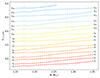 |
Fig. 12. Evolution of the ℓ = 1 modes with mass. Each point represents the frequency of the mode with the indicated radial order (obtained through interpolation) for the model with the given mass at the position in the evolutionary track corresponding to ρc = 16 000 g.cm−3. |
To further understand the anomaly, we consider a smaller and denser subgrid purposely built to further explore this problem. This denser subgrid considers the exact same physics as the main grid described in Section 3, only with different mass inputs (that vary between 1.170 and 1.180 M⊙, in steps of 0.001 M⊙). Figure 13 shows the evolution of ν1, 11, norm with ρc for the different mass tracks of such subgrid, zoomed in on a middle stage of the subgiant phase (in the interval ρc = [13000, 18 000] g.cm−3, or equivalently, τscaled = [0.890, 0.925]). We can see that increasing the grid resolution in mass step worsens the problem, since the curves describing the evolution of the mode frequency along the evolutionary tracks with masses 1.176 and 1.177 M⊙ are further apart than those corresponding to the masses of M = 1.175 and 1.180 M⊙. Thus, the problem presented in Figure 11 cannot be solved by increasing the grid resolution in a specific region of the parameter space of the grid. This is more prominently displayed in Figure 14, where the results of applying the full interpolation algorithm to this denser subgrid, namely to the track with M = 1.177 M⊙, show no clear improvement.
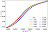 |
Fig. 13. Evolution of the mode frequency ν1, 11, norm along an avoided crossing taking place at central densities between ρc = 13 000 and 18 000 g.cm−3 for the models of the stellar subgrid with fov = 0.01. The transition mass between radiative and convective cores in the MS is 1.176 M⊙ for this choice of fov. |
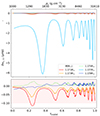 |
Fig. 14. Interpolation errors presented as a function of τscaled (bottom x-axis) and ρc (top x-axis), that resulted from the application of the full interpolation algorithm (cubic splines along tracks and linear across tracks). Results are shown for all ν1, 11 mode frequencies of the subgrid of stellar models with fov = 0.01, when ρc is the age proxy for interpolation. The transition mass, between radiative and convective cores in the MS, is 1.176 M⊙ for this choice of fov. The bottom subplot presents a zoom in on the results of interpolation of the top subplot for δν1, 11 between −0.14 and 0.04 μHz. |
Considering the dependence of the avoided crossings on the core conditions (cf. Section 2), we conjecture that the discontinuity discussed above could be a result of different core properties associated with stellar models with different masses, since these mass values are typically associated with a transition between stars that had either a radiative core or a convective core during their MS. This conjecture is supported by the evolution of the mass of the convective core in our grid, during the corresponding MS stages. For evolutionary tracks with M ≤ 1.175 M⊙, the mass of the convective core is non zero at the beginning of the MS, but it quickly becomes zero, remaining zero until the end of the MS. However, for M ≥ 1.175 M⊙, the convective core mass is positive for most of the MS stage. This demonstrates a clear relation between the structure of the star during its MS and the systematic interpolation errors observed during the subgiant phase.
To investigate further the relation between the core structure and the interpolation errors, and explore possible ways to mitigate the problem, we consider the impact of the adopted core physics, in particular, the overshoot. In particular, we consider a new subgrid, with similar physics as the main grid described in Section 3, but where we turn off the convective overshoot, by setting fov = 0.00. Such a decrease in fov also implies a change in the transitional mass at which stars begin to develop a convective core. Thus, we consider different mass inputs for this subgrid (varying between 1.180 and 1.190 M⊙), as we find the transitional mass for the case with no overshoot to be located between 1.182 and 1.183 M⊙.
Figure 15 shows the evolution of the mode frequency ν1, 11, norm with central density ρc for the case with no convective overshoot, zoomed in on the same stage of the subgiant evolution as in Figure 13. The discontinuity essentially disappears when fov is set to zero. This shows that the cause of the discontinuity is not the appearance of a sustained convective core during the MS per se, but rather the abrupt change in the extent of the core across masses when an overshoot layer characterised by a fixed value of fov is added at the core edge, using the current overshoot formulation. In fact, inspection of our models with overshoot shows that the abrupt change in core conditions when crossing the transition mass leads to a discontinuity in central temperature, Tc, at fixed ρc. This is then reflected in a jump in the frequencies of a given mode across the same mass transition. To avoid this, it may be useful to consider as an age proxy the quantity ρc2μc/Tc (cf. Equation 3), in place of ρc.
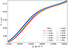 |
Fig. 15. Evolution of the mode frequency ν1, 11, norm along an avoided crossing taking place at central densities between ρc = 13 000 and 18 000 g.cm−3 for the models of the stellar subgrid with fov = 0.00. The transition mass, between radiative and convective cores in the MS, is 1.182 M⊙ for this choice of fov. |
The results of applying the full interpolation method to this second subgrid are presented in Figure 16. In this case, the interpolation errors associated with the transitional mass (which corresponds to the interpolated mass track with M = 1.183 M⊙) are no longer atypically large, with the maximum error being 8.9 × 10⁻² μHz, well below the set accuracy limit of 0.1 μHz.
 |
Fig. 16. Interpolation errors presented as a function of τscaled (bottom x-axis) and ρc (top x-axis) that resulted from the application of the full interpolation algorithm (cubic splines along tracks and linear across tracks). Results are shown for all ν1, 11 mode frequencies of the subgrid of stellar models with fov = 0.00, when ρc is the age proxy for interpolation. The transition mass, between radiative and convective cores in the MS, is 1.182 M⊙ for this choice of fov. |
Turning off fov may not be the adequate way to mitigate the interpolation problem in this region of the grid, since this parameter describes important physics that affects the stellar structure of the subgiants. Still, these results show the importance of either ensuring that the grid is built such as to minimise the impact of abrupt structural changes on interpolation, or, in cases where there is no adequate way of doing that, accounting for the additional errors that may result from interpolation. In the specific case of core overshoot, a possible alternative is to consider a mass dependent overshoot, as suggested by Claret & Torres (2018), based on a study of eclipsing binaries. Such smooth variation in overshoot near the transition mass could potentially also mitigate the problem detected here.
6. Conclusions
In this work, we performed a detailed study of classical interpolation algorithms applied to a grid of stellar models in the subgiant phase. Our primary goal was to verify whether these algorithms ensure the computation of the ℓ = 1 mode frequencies with interpolation errors within the typical observational errors (∼0.1 μHz). The study was applied to a grid of 41 evolutionary tracks, varying only in stellar mass between 1.150 and 1.350 M⊙, separated by steps of 0.005 M⊙, chosen to cover the mass transition where their MS progenitors start to develop a sustained convective core. All other inputs were fixed, including the convective overshooting parameter, set to fov = 0.01 in our initial grid. As a second goal, the work aimed at establishing the procedure, among those tested, that produces the smallest average offsets (for all modes, over evolution) and the smallest maximum absolute errors on the interpolated frequencies.
We tested different variations of the two-step interpolation algorithm, which considered various order methods (linear and cubic splines) and different age proxies (physical age, τ, scaled age, τscaled, and central density, ρc). We applied the algorithm to a grid with typical resolution in mass and age. Our main conclusions are as follows: 1) The accuracy goal is not satisfied in any of the configurations considered, with the maximum interpolation error easily surpassing the reference accuracy limit of 0.1 μHz by at least an order of magnitude. 2) The best results are obtained with the interpolation algorithm that considers cubic spline interpolation along evolutionary tracks, linear interpolation across evolutionary tracks, and ρc as the age proxy. This interpolation algorithm yielded average offsets within twice the reference limit, but maximum errors up to an order of magnitude higher than that. These results show that the identification of an age proxy that is fully appropriate for the interpolation of mode frequencies in the presence of avoided crossings remains an open problem.
We also varied the density of models in the grid, starting with about 1500 models per evolutionary track to be used in interpolation, and decreasing such number progressively to 1/6 of that value, and investigated how the grid resolution influences the interpolation results. We established that reducing the number of models per evolutionary track to 1/3 of the initial value (∼500 models) does not significantly change the results, with the average offset remaining within twice the accuracy limit. This seems to establish a minimal number of models per subgiant evolutionary track within the grid paradigm considered here, allowing future works to focus on larger ranges of stellar masses when building stellar grids, and additional input parameters, such as metallicity, [Fe/H], and convective overshoot, fov. Such a grid could be used, e.g. for a reevaluation of the studies performed so far on Kepler subgiants data. Nevertheless, we emphasise that, in all cases, the maximum errors across the grid are well above the established goal, and that regions in the grid in which the stellar structure varies abruptly are subject to even larger and systematic interpolation errors.
The work presented here is important in the context of space missions collecting asteroseismic data to characterise stars, such as PLATO, whose pipelines may rely on the use of stellar models. Our work indicates that, in the subgiant phase, state-of-the-art interpolation approaches in typical stellar grids will not enable the exploitation to their full potential of the exquisite seismic data that will be acquired. This, in turn, points to the need of developing a new generation of interpolation algorithms that may mitigate the problems identified in this work.
In addition to cubic splines, we tested the grid resolution using interpolation with cubic polynomials, for which we expect the errors to increase as k4. As we found that not to be the case, we made a sanity test on an evolutionary track with 10 times the number of models of the initial grid and we found out that our interpolation routine does produce errors that increase with the expected scaling, implying that the reason this does not happen here is because our grid is not sufficiently dense to be in such regime.
Acknowledgments
This work was supported by Fundação para a Ciência e a Tecnologia (FCT/MCTES) through national funds by grants UIDB/04434/2020 (DOI: 10.54499/UIDB/04434/2020), UIDP/04434/2020 (DOI: 10.54499/UIDP/04434/2020), 2022.06962.PTDC, and 2022.03993.PTDC (DOI:10.54499/2022.03993.PTDC). MC is supported by FCT through a grant with reference 2020.07530.BD. MSC and TLC are supported by FCT through work contracts CEECIND/02619/2017 and CEECIND/00476/2018, respectively. SD acknowledges support from the project BEAMING ANR-18-CE31-0001 of the French National Research Agency (ANR) and from the Centre National d’Études Spatiales (CNES).
References
- Aerts, C., Christensen-Dalsgaard, J., & Kurtz, D. W. 2010, Asteroseismology (Springer Science+Business Media B.V.) [Google Scholar]
- Aguirre Børsen-Koch, V., Rørsted, J. L., Justesen, A. B., et al. 2022, MNRAS, 509, 4344 [Google Scholar]
- Asplund, M., Grevesse, N., Sauval, A. J., & Scott, P. 2009, ARA&A, 47, 481 [NASA ADS] [CrossRef] [Google Scholar]
- Baglin, A., Auvergne, M., Boisnard, L., et al. 2006, 36th COSPAR Scientific Assembly, 3749 [Google Scholar]
- Balser, D. S. 2006, AJ, 132, 2326 [Google Scholar]
- Böhm-Vitense, E. 1958, Z. Astrophys., 46, 108 [Google Scholar]
- Campante, T. L., Schofield, M., Kuszlewicz, J. S., et al. 2016, ApJ, 830, 138 [Google Scholar]
- Claret, A., & Torres, G. 2018, ApJ, 859, 100 [Google Scholar]
- Cox, J. P., & Giuli, R. T. 1968, Principles of stellar structure (New York: Gordon and Breach) [Google Scholar]
- Cunha, M. S. 2018, Astrophys. Space Sci. Proc., 49, 27 [NASA ADS] [CrossRef] [Google Scholar]
- Cunha, M. S., Antoci, V., Holdsworth, D. L., et al. 2019, MNRAS, 487, 3523 [NASA ADS] [CrossRef] [Google Scholar]
- Cunha, M. S., Roxburgh, I. W., Aguirre Børsen-Koch, V., et al. 2021, MNRAS, 508, 5864 [NASA ADS] [CrossRef] [Google Scholar]
- Cyburt, R. H., Fields, B. D., & Olive, K. A. 2003, Phys. Lett. B, 567, 227 [NASA ADS] [CrossRef] [Google Scholar]
- Deheuvels, S., & Michel, E. 2011, A&A, 535, A91 [NASA ADS] [CrossRef] [EDP Sciences] [Google Scholar]
- Ferguson, J. W., Alexander, D. R., Allard, F., et al. 2005, ApJ, 623, 585 [Google Scholar]
- Fossat, E., Boumier, P., Corbard, T., et al. 2017, A&A, 604, A40 [NASA ADS] [CrossRef] [EDP Sciences] [Google Scholar]
- Garcia, R. A., Ballot, J., Eff-Darwich, A., et al. 2010, ArXiv e-prints [arXiv:1007.4445] [Google Scholar]
- Gilliland, R. L., Brown, T. M., Christensen-Dalsgaard, J., et al. 2010, PASP, 122, 131 [Google Scholar]
- Goupil, M. J., Catala, C., Samadi, R., et al. 2024, A&A, 683, A78 [NASA ADS] [CrossRef] [EDP Sciences] [Google Scholar]
- Grevesse, N., & Sauval, A. J. 1998, Space Sci. Rev., 85, 161 [Google Scholar]
- Herwig, F. 2000, A&A, 360, 952 [NASA ADS] [Google Scholar]
- Imbriani, G., Costantini, H., Formicola, A., et al. 2005, Eur. Phys. J. A, 25, 455 [Google Scholar]
- Koch, D. G., Borucki, W. J., Basri, G., et al. 2010, ApJ, 713, L79 [Google Scholar]
- Krishna Swamy, K. S. 1966, ApJ, 145, 174 [Google Scholar]
- Kunz, R., Fey, M., Jaeger, M., et al. 2002, ApJ, 567, 643 [CrossRef] [Google Scholar]
- Lebreton, Y., & Reese, D. R. 2020, A&A, 642, A88 [NASA ADS] [CrossRef] [EDP Sciences] [Google Scholar]
- Li, T., Bedding, T. R., Kjeldsen, H., et al. 2019, MNRAS, 483, 780 [Google Scholar]
- Li, T., Bedding, T. R., Christensen-Dalsgaard, J., et al. 2020, MNRAS, 495, 3431 [Google Scholar]
- Mosser, B., Elsworth, Y., Hekker, S., et al. 2012, A&A, 537, A30 [NASA ADS] [CrossRef] [EDP Sciences] [Google Scholar]
- Nsamba, B., Campante, T. L., Monteiro, M. J. P. F. G., et al. 2018, MNRAS, 477, 5052 [NASA ADS] [CrossRef] [Google Scholar]
- Nsamba, B., Moedas, N., Campante, T. L., et al. 2021, MNRAS, 500, 54 [Google Scholar]
- Paxton, B., Bildsten, L., Dotter, A., et al. 2011, ApJS, 192, 3 [Google Scholar]
- Paxton, B., Cantiello, M., Arras, P., et al. 2013, ApJS, 208, 4 [Google Scholar]
- Paxton, B., Marchant, P., Schwab, J., et al. 2015, ApJS, 220, 15 [Google Scholar]
- Paxton, B., Schwab, J., Bauer, E. B., et al. 2018, ApJS, 234, 34 [NASA ADS] [CrossRef] [Google Scholar]
- Paxton, B., Smolec, R., Schwab, J., et al. 2019, ApJS, 243, 10 [Google Scholar]
- Planck Collaboration XIII. 2016, A&A, 594, A13 [NASA ADS] [CrossRef] [EDP Sciences] [Google Scholar]
- Rauer, H., Catala, C., Aerts, C., et al. 2014, Exp. Astron., 38, 249 [Google Scholar]
- Rauer, H., Heras, A., Mas-Hesse, M., & Pagano, I. 2023, AAS/Div. Planet. Sci. Meeting Abstr., 55, 31901 [Google Scholar]
- Rendle, B. M., Buldgen, G., Miglio, A., et al. 2019, MNRAS, 484, 771 [Google Scholar]
- Ricker, G. R., Winn, J. N., Vanderspek, R., et al. 2015, J. Astron. Telescopes Instrum. Syst., 1, 014003 [Google Scholar]
- Rodrigues, T. S., Bossini, D., Miglio, A., et al. 2017, MNRAS, 467, 1433 [NASA ADS] [Google Scholar]
- Townsend, R. H. D., & Teitler, S. A. 2013, MNRAS, 435, 3406 [Google Scholar]
- Unno, W., Osaki, Y., Ando, H., Saio, H., & Shibahashi, H. 1989, Nonradial oscillations of stars (Tokyo: University of Tokyo Press) [Google Scholar]
Appendix A: Interpolation errors resulting from the full interpolation algorithm
The following table of tables presents the average offset (μ) and maximum error (m) (in μHz) from the full interpolation method, which considers cubic splines along evolutionary tracks and the indicated interpolation method across evolutionary tracks, for all ℓ = 1 modes obtained for the interpolated tracks of the initial grid, with the interpolated mass value indicated on the top-left cell of each table.
Average offset (μ) and maximum errors (m) for different age proxies.
All Tables
All Figures
|
Fig. 1. Evolution of the normalised frequencies of non-radial ℓ = 1 modes, with radial order n = 11, for evolutionary tracks of a stellar grid (the details of which are given in Section 3) with masses between 1.23 and 1.27 M⊙, as a function of the physical age τ (top) and the central density ρc (bottom). The points connected by a dashed line in the top panel indicate models with an age of 4.18 Gyr. The bottom panel displays a subplot that zooms on a particular avoided crossing for the mass M = 1.24 M⊙. |
| In the text | |
|
Fig. 2. Hertzsprung–Russell diagram displaying every tenth model of each of the 41 tracks in the subgiant phase produced for the stellar grid described in the text. |
| In the text | |
|
Fig. 3. Interpolation errors presented as a function of τscaled (bottom x-axis) and ρc (top x-axis) that resulted from interpolation along the evolutionary track with M = 1.245 M⊙ for all ℓ = 0 frequency modes, with radial orders n ∈ [9, 23] indicated by different colours. Each subplot presents the results for a different interpolation method, considering different methods – linear (top panels) or cubic splines (bottom panels) – and different age proxies – τscaled (left) and ρc (right). |
| In the text | |
|
Fig. 4. Interpolation errors presented as a function of τscaled (bottom x-axis) and ρc (top x-axis) that resulted from interpolation along the evolutionary track with M = 1.245 M⊙ for all ℓ = 1 frequency modes, with radial orders n ∈ [1, 20] indicated by different colours. Each subplot presents the results for a different interpolation method, namely linear (top panels) and cubic splines (bottom panels), and different age proxies – τscaled (left) and ρc (right). |
| In the text | |
|
Fig. 5. Interpolation errors presented as a function of τscaled (bottom x-axis) and ρc (top x-axis) that resulted from the full interpolation algorithm (cubic splines interpolation along tracks, and linear interpolation across tracks) for all ℓ = 0 modes associated with the mass track M = 1.245 M⊙ when considering τ (top), τscaled (middle) and ρc (bottom) as the age proxies for interpolation. |
| In the text | |
|
Fig. 6. Interpolation errors presented as a function of τscaled (bottom x-axis) and ρc (top x-axis) that resulted from the full interpolation algorithm (cubic splines interpolation along tracks, and linear interpolation across tracks) for all ℓ = 1 modes associated with the track with M = 1.245 M⊙ when considering τ (top), τscaled (middle) and ρc (bottom) as the age proxies for interpolation. |
| In the text | |
|
Fig. 7. Interpolation errors presented as a function of τscaled (bottom x-axis) and ρc (top x-axis) that resulted from the full interpolation algorithm (cubic splines interpolation both along and across tracks) for all ℓ = 1 modes associated with the track with M = 1.245 M⊙ when considering τ (top), τscaled (middle) and ρc (bottom) as the age proxies for interpolation. |
| In the text | |
|
Fig. 8. Evolution of the scaled frequencies for the ℓ = 0 modes, with radial order n = 11, that resulted from applying the interpolation algorithm to the mass track with M = 1.245 M⊙, presented as a function of τ (top) and τscaled (bottom), when each is considered as the respective age proxy for interpolation. The bottom panel displays a subplot that zooms on the region of the age proxy parameter space with the highest interpolation errors. |
| In the text | |
|
Fig. 9. Evolution of the normalised frequencies of non-radial ℓ = 1 modes with radial orders n = [10, 11, 12] for evolutionary tracks of the stellar grid with masses between 1.23 and 1.26 M⊙ as a function of the various age proxies considered for interpolation: τ (left), τscaled (middle), and ρc (right). Different colours are used to represent different stellar masses and different line styles show different radial orders, according to the insets in the middle and right panel, respectively. |
| In the text | |
|
Fig. 10. Average offsets (μ, indicated by squares; in μHz) and maximum errors (m, indicated by triangles; in μHz) from the full interpolation method, which considers cubic splines along evolutionary tracks and linear (top) or cubic splines (bottom) interpolation across evolutionary tracks and τscaled (red) or ρc (yellow) as the age proxy, for all ℓ = 1 modes obtained for the interpolated tracks of the initial grid. The vertical brown dotted line highlights the results for our reference track with M = 1.245 M⊙, while the vertical brown dashed line highlights the anomalous track with M = 1.175 M⊙. |
| In the text | |
|
Fig. 11. Interpolation errors presented as a function of τscaled (bottom x-axis) and ρc (top x-axis) that resulted from the application of the full interpolation algorithm (cubic splines along tracks and linear across tracks) across the complete grid. Results are shown for all ν1, 11 mode frequencies, when ρc is considered as the age proxy for interpolation. The transition mass, between radiative and convective cores in the MS, is 1.175 M⊙ for this choice of fov. The bottom subplot zooms on the results for interpolation presented in the top subplot for δν1, 11 between −1.2 and 1.4 μHz. |
| In the text | |
|
Fig. 12. Evolution of the ℓ = 1 modes with mass. Each point represents the frequency of the mode with the indicated radial order (obtained through interpolation) for the model with the given mass at the position in the evolutionary track corresponding to ρc = 16 000 g.cm−3. |
| In the text | |
|
Fig. 13. Evolution of the mode frequency ν1, 11, norm along an avoided crossing taking place at central densities between ρc = 13 000 and 18 000 g.cm−3 for the models of the stellar subgrid with fov = 0.01. The transition mass between radiative and convective cores in the MS is 1.176 M⊙ for this choice of fov. |
| In the text | |
|
Fig. 14. Interpolation errors presented as a function of τscaled (bottom x-axis) and ρc (top x-axis), that resulted from the application of the full interpolation algorithm (cubic splines along tracks and linear across tracks). Results are shown for all ν1, 11 mode frequencies of the subgrid of stellar models with fov = 0.01, when ρc is the age proxy for interpolation. The transition mass, between radiative and convective cores in the MS, is 1.176 M⊙ for this choice of fov. The bottom subplot presents a zoom in on the results of interpolation of the top subplot for δν1, 11 between −0.14 and 0.04 μHz. |
| In the text | |
|
Fig. 15. Evolution of the mode frequency ν1, 11, norm along an avoided crossing taking place at central densities between ρc = 13 000 and 18 000 g.cm−3 for the models of the stellar subgrid with fov = 0.00. The transition mass, between radiative and convective cores in the MS, is 1.182 M⊙ for this choice of fov. |
| In the text | |
|
Fig. 16. Interpolation errors presented as a function of τscaled (bottom x-axis) and ρc (top x-axis) that resulted from the application of the full interpolation algorithm (cubic splines along tracks and linear across tracks). Results are shown for all ν1, 11 mode frequencies of the subgrid of stellar models with fov = 0.00, when ρc is the age proxy for interpolation. The transition mass, between radiative and convective cores in the MS, is 1.182 M⊙ for this choice of fov. |
| In the text | |
Current usage metrics show cumulative count of Article Views (full-text article views including HTML views, PDF and ePub downloads, according to the available data) and Abstracts Views on Vision4Press platform.
Data correspond to usage on the plateform after 2015. The current usage metrics is available 48-96 hours after online publication and is updated daily on week days.
Initial download of the metrics may take a while.