| Issue |
A&A
Volume 693, January 2025
|
|
|---|---|---|
| Article Number | A148 | |
| Number of page(s) | 9 | |
| Section | Astronomical instrumentation | |
| DOI | https://doi.org/10.1051/0004-6361/202452159 | |
| Published online | 13 January 2025 | |
Validation of millimetre and sub-millimetre atmospheric collision-induced absorption at Chajnantor
1
Consejo Superior de Investigaciones Cientifícas, Instituto de Física Fundamental,
Calle Serrano 121,
28006
Madrid,
Spain
2
European Southern Observatory,
Karl-Schwarzschild-Str. 2,
85748
Garching,
Germany
3
Max-Planck-Institut für Radioastronomie,
Auf dem Hügel 69,
53121
Bonn,
Germany
4
European Southern Observatory,
Alonso de Córdova 3107, Vitacura Casilla
7630355,
Santiago,
Chile
5
Centre National de la Recherche Scientifique, Observatoire de Paris, Laboratoire d’Etudes du Rayonnement et la Matière en Astrophysique,
77 Avenue Denfert Rochereau,
75014
Paris,
France
6
Jet Propulsion Laboratory, California Institute of Technology,
4800 Oak Grove Drive,
Pasadena,
CA
91109,
USA
7
Centro de Astro-Ingeniería UC, Instituto de Astrofísica, Pontificia Universidad Católica de Chile,
Avda Vicuña Mackenna 4860,
Macul, Santiago,
Chile
8
Departamento de Física de la Tierra y Astrofísica e Instituto de Física de Partículas y del Cosmos (IPARCOS). Universidad Complutense de Madrid, Ciudad Universitaria,
28040
Madrid,
Spain
★ Corresponding author; This email address is being protected from spambots. You need JavaScript enabled to view it.
Received:
6
September
2024
Accepted:
18
November
2024
Abstract
Due to the importance of a reference atmospheric radiative transfer model for both planning and calibrating ground-based observations at millimetre and sub-millimetre wavelengths, we have undertaken a validation campaign consisting of acquiring atmospheric spectra under different weather conditions, in different diurnal moments and seasons, with the Atacama Pathfinder EXperiment (APEX), due to the excellent stability of its receivers and the very high frequency resolution of its back-ends. As a result, a dataset consisting of 56 spectra within the 157.3–742.1 GHz frequency range, at kilohertz resolution (smoothed to ∼2–10 MHz for analysis), and spanning one order of magnitude (∼0.35–3.5 mm) in precipitable water vapour columns, has been gathered from October 2020 to September 2022. These data are unique for their quality and completeness and, due to the proximity of APEX to the Atacama Large Millimeter/Submillimeter Array (ALMA), they provide an excellent opportunity to validate the atmospheric radiative transfer model currently installed in the ALMA software. The main issues addressed in the study are possible missing lines in the model, line shapes, vertical profiles of atmospheric physical parameters and molecular abundances, seasonal and diurnal variations, and collision-induced absorption (CIA), to which this paper is devoted, in its N2–N2 + N2–O2 + O2–O2 (dry) and N2–H2O + O2 –H2O (‘foreign’ wet) mechanisms. All these CIA terms should remain unchanged in the above-mentioned ALMA atmospheric model as a result of this work.
Key words: atmospheric effects / site testing / techniques: spectroscopic
© The Authors 2025
 Open Access article, published by EDP Sciences, under the terms of the Creative Commons Attribution License (https://creativecommons.org/licenses/by/4.0), which permits unrestricted use, distribution, and reproduction in any medium, provided the original work is properly cited.
This article is published in open access under the Subscribe to Open model. This email address is being protected from spambots. You need JavaScript enabled to view it. to support open access publication.
1 Introduction
Millimetre- and sub-millimetre-wavelength observations of cold dark clouds, star-forming regions, evolved stars, galaxies, and other objects in space have broadened our vision of the Universe over the last few decades. These observations are usually performed from high and dry sites, where conditions offering some sky transparency for them are found, as Hills et al. (1978) revealed with pioneering site testing observations from Tenerife at ~2400 meters above sea level. Even so, the atmospheric millimetre and sub-millimetre spectrum is rather complicated and fast-changing, both in space and time. Site testing for ground-based sub-millimetre observatories and field spectroscopy and radiometry experiments continued over the years in the Atacama Desert (Chile), Hanle (India), the Tibetan Plateau, Greenland, the South Pole, Mauna Kea (Hawai’i), and a few other sites. The work presented here is a continuation of the Mauna Kea studies of Pardo et al. (2001a) and Pardo et al. (2005), as it uses their resulting atmospheric radiative transfer model (Pardo et al. 2001b) as the starting point (for a wider view on the subject, see a 2012 review in Tremblin et al. (2012) and several complementary publications from the last 25 years, such as Matsushita et al. (1999), Paine et al. (2000), Chamberlin et al. (2003), Ji et al. (2004), Shi at al. (2016), Matsushita et al. (2017), Mlawer et al. (2019), Ningombam et al. (2020), Pardo et al. (2022), and Mlawer et al. (2023).
The contributors to the millimetre and sub-millimetre atmospheric spectrum are O2 through magnetic dipolar (M1) rotational transitions, H2O through electric dipolar (E1) rotational transitions, weaker E1 features from other ‘minor’ atmospheric gases, such as N2O, CO, HCN, HCl, and O3 and its isotopo-logues and vibrationally excited states, and, finally, non-resonant collision-induced absorption (CIA) due to several mechanisms: N2–N2, O2–O2, and O2–N2 collisions (dry CIA), H2O–N2 + H2O–O2 collisions (‘foreign’ wet CIA), and H2O–H2O collisions (‘self’ wet CIA). This last term is almost two orders of magnitude lower than the foreign CIA in the dry conditions (a precipitable water vapour column (PWVC) of <2mm) relevant to observations at frequencies above approximately 170 GHz, and therefore does not play a role in this study.
The importance of a reference atmospheric radiative transfer model for both planning and contributing in the calibration of ground-based observations at millimetre and sub-millimetre wavelengths is the main motivation of this study. From 2006 to 2011, the C++ implementation of the Pardo et al. (2001b) atmospheric transmission model (ATM) was achieved, under European Southern Observatory (ESO) contract 14977/ESO/07/15694/YWE, to the Telescope Calibration subsystem (TelCal) of the official ALMA software. ATM includes the spectroscopy and reference vertical profiles for all relevant molecular species contributing to the millimetre and sub-millimetre atmospheric spectrum seen from ground-based observatories, along with empirical and theoretical descriptions of the CIA mechanisms. The software was delivered on schedule and has been used within ALMA since the first cycle of science observations. Figure 1 shows a reference calculation of the different opacity terms in ATM under typical conditions at the APEX site on the Chajnantor Plateau, assuming internal model parameters as in Sect. 5. The dry opacity component (dark blue, light blue, and pink lines in the figure) is quite constant at the site, with maximum variations of just a few percent. However, the wet part of the opacity (black and red lines in the figure) has a dynamic range of more than one order of magnitude, even in clear sky conditions, and significant changes can be expected on timescales as short as a few minutes.
Figure 1 shows the importance of CIA absorption for the total atmospheric opacity and brightness temperature. For example, the foreign wet CIA exceeds the H2O lines opacity for most of the ~205–302 GHz range and this translates into the large effect of removing it in the model seen in Fig. 4. The CIA terms also explain that the atmospheric transmission in sub-millimetre windows is not as good as a simple ‘lines only’ model would predict. For this reason, the validation of atmospheric CIA terms is very important for millimetre and sub-millimetre observatories, and is the main motivation of this paper.
Besides astronomy, the study of CIA terms is also of interest for Earth observations and the remote sensing community. Current operational meteorological applications are limited to 200 GHz. The upcoming EUropean organisation for the exploitation of METeorological SATellites (EUMETSAT) Polar System-Second Generation (MetOp-SG), to be launched in 2025, will carry an instrument, the Ice Cloud Imager (ICI), with frequencies up to 664 GHz (Klein et al. 2016). The main objective of ICI is to provide data on humidity and ice hydrometeors, particularly the bulk ice mass that can be uniquely quantified with millimetre wave observations from satellites. Furthermore, the deployment of the EUMETSAT Polar System – Sterna (EPS-Sterna) constellation, consisting of six micro-satellites for launch around 2030, will enhance numerical weather prediction (NWP) accuracy. Each micro-satellite will carry a sounder, including channels around the H2O line at 325 GHz, providing global temperature and water vapour profiles with unparalleled coverage and revisit times. The fast radiative transfer models used for satellite data assimilation in NWP models are based on atmospheric line-by-line spectroscopy and on the so-called MT-CKD (Mlawer-Tobin-Clough-Kneizys-Davies) water vapour CIA (Mlawer et al. 2019, Mlawer et al. 2023). The MT-CKD is primarily tuned for Earth’s energy budget, and as a consequence focusses mainly on frequencies higher than 3 THz, as frequencies below are only weakly contributing to the surface or top-of-atmosphere energy budgets. The carefully calibrated APEX observations presented in this work provide additional constraints to the water vapour CIA, to validate existing models in the millimetre and sub-millimetre wave ranges.
Most site testing and model validation campaigns at millimetre and sub-millimetre wavelengths have been carried out with broadband (several hundreds of GHz) Fourier transform spectrometers, with frequency resolutions ranging from ~0.2 to 10 GHz, and tipping radiometers using ‘window’ frequencies such as 220, 225, 492, or 850 GHz (see previous references in this section). Our study is the first to offer broadband coverage (several hundred gigahertz) and very high spectral resolution (better than 1 MHz), although this last aspect is not critical for CIA validation and we have smoothed the resolution to ~10 MHz. The original resolution, however, will be preserved in future papers in order to focus on the fine details of the atmospheric spectrum such as line shapes and very weak spectral features. Section 2 presents the telescope, receivers, and the instrumental set-up. A crucial update on the calibration, with respect to our previous Pardo et al. (2022) work, can be found in Sect. 3. The observing runs are described in Sect. 4 along with the useful spectra that will be used for the detailed analysis presented in Sect. 5. The output from this analysis leads to a discussion in Sect. 6 that will focus on the role of CIA, and far-wings of supra-THz H2O lines, in the atmospheric spectrum. Summary and conclusions are given in Sect. 7.
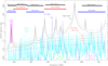 |
Fig. 1 Reference ATM model for the APEX site, considering 555 hPa and 273 K as physical parameters at the ground, and 0.5 (dotted black and red lines), 1.0 (solid black and red lines), and 2.0 mm (dashed black and red lines) of the PWVC. Note that the H2O–H2O (self wet) CIA is in practice negligible in these very dry conditions (only the curve for 2.0 mm PWVC is shown in a dashed green colour as the curves for 1.0 and 0.5 mm PWVC are below the bottom Y limit of the plot). The frequency ranges covered by the SEPIA and nFLASH receivers used in this work are plotted for reference, as are ALMA bands 5–9. The central frequencies of the six double side-band channels of the APEX WVR, on both sides of the 183.31 GHz H2O line, are also plotted. The red and pink ClA curves are the ones under validation in this paper. Cyan (minor gases opacity), blue (O2 lines opacity) and pink (dry CIA opacity) curves remain unchanged for all PWVC values. |
2 Instrumental set-up
The Atacama Pathfinder EXperiment (APEX) (Güsten et al. 2006) is a world-class millimetre and sub-millimetre observatory operating at a distance of roughly 2 km from the centre of ALMA, on the Chajnantor Plateau in the Chilean Andes, 5105 meters above sea level. It hosts a large variety of instruments, from several European partners, due to the experimental nature of this project. The APEX antenna has a diameter of 12 meters and is made of 264 aluminium panels. The full surface accuracy is better than 15 µm root mean square. Among the different instruments available, there are five sideband-separating (2SB) heterodyne (Het) superconductor–insulator–superconductor (SIS) tunnel junction receivers that have been used for this project, connected to fast Fourier transform spectrometers (FFTSs) providing kilohertz spectral resolutions. The good performance of them for our goals, and the proximity to ALMA, provide an excellent opportunity to validate the atmospheric model used in the latter facility, but also in APEX and other millimetre and sub-millimetre observatories around the world.
A first set of receivers, called SEPIA for the Swedish ESO PI Instrument at APEX, are in a cryostat that can accommodate three ALMA-like receiver cartridges with tertiary optics to illuminate them inside the Nasmyth cabin A of the APEX telescope. They were designed, constructed, and installed by the Group for Advanced Receiver Development (GARD) at Onsala Space Observatory (OSO) in Sweden. The SEPIA cryostat was also manufactured by the GARD team. A complete technical description can be found in Belitsky et al. (2018), for SEPIA180 and SEPIA660, and Meledin et al. (2022) for SEPIA345. SEPIA660 was used in our previous Pardo et al. (2022) publication.
SEPIA180 (159–211 GHz) is a dual polarisation 2SB receiver built to the specifications of ALMA Band 5 (it is based on the pre-production version of such a receiver). It has two intermediate frequency (IF) outputs per polarisation, upper and lower sidebands (USB and LSB), each covering 4–8 GHz, adding up a total of 16 GHz instantaneous IF bandwidth. The central frequencies of the two sidebands are separated by 12 GHz. The sideband rejection ratio is by design >10 dB and 18.5 dB on average. The single-sideband noise temperature is below 55 K at all frequencies within the band.
SEPIA345 (272-376 GHz) is a dual polarisation 2SB receiver delivered in 2020. It has two IF outputs per polarisation, USB and LSB, each covering 4–12 GHz, adding up a total of 32 GHz instantaneous IF bandwidth. The central frequencies of the two sidebands are separated by 16 GHz. Each sideband (and polarisation) is recorded by two FFTS spectrometer units, each of them sampling 4 GHz in the following configuration: FFTS1, in the 4.17–8.17 GHz IF bandwidth, and FFTS2, in the 8.07–12.07 GHz IF bandwidth. Therefore, both units overlap in the middle for about 100 MHz and the full coverage is slightly smaller than 8 GHz (7.9 GHz). The sideband rejection ratio is by design >10 dB over 90% of the band. Typical values of receiver temperature are < 100 K below 320 GHz, approach 150 K at 340 GHz, and then rise towards the high-frequency end of the receiver band.
SEPIA660 (597–725 GHz) is a dual polarisation 2SB receiver that was installed and commissioned during the second half of 2018. The rest of the characteristics are as for SEPIA345 with the exception of the receiver temperature, which is below 350 K at all frequencies within the band and below 250 K in the central part of it.
The other bands (nFLASH) were delivered in 2020 by the MPIfR Sub-mm technology division in Bonn. It is a receiver with two independently tunable frequency channels: nFLASH230 and nFLASH460. Both channels are dual polarisation (two SIS mixers per channel) and sideband-separating (2SB), meaning four SIS junctions in total. The instrument is designed to work as a dual colour receiver to allow for simultaneous observing in both channels.
nFLASH230 (188–282 GHz) has an extended IF coverage, from 4 to 12 GHz, and therefore it covers up to a total of 32 GHz IF instantaneous bandwidth including both sidebands and polarisations. The separation between the centre of the two sidebands is 16 GHz. Each sideband (and polarisation) is recorded by two spectrometer processors units (FFTSs), each of them recording 4 GHz in the following configuration: FFTS1 in the 4.17 – 8.17 GHz IF bandwidth, and FFTS2 in the 8.07–12.07 GHz IF bandwidth. Therefore, both units overlap in the middle for about 100 MHz and the full coverage is slightly smaller than 8 GHz (7.9 GHz). The typical receiver temperature is 60–80 K, increasing up to 80-90 K at the extremes of the frequency window (below 210 GHz or above 260 GHz LO frequencies). The sideband rejection is typically around 15 dB.
nFLASH460 (377–508 GHz) has a 4–8 GHz output IF bandwidth, which is half the bandwidth that is covered by the nFLASH230 channel. The separation between the centre of the two sidebands is 12 GHz and each sideband (and polarisation) is covered by one FFTS spectrometer unit of 4 GHz bandwidth. The receiver temperatures are typically below 150 K, except at the high-frequency end of the spectral window (LO frequency > 480 GHz) where this increases to higher values. Sideband rejection is typically better than 15 dB all over the band.
Some spectra obtained in this work with these five receivers can be seen in Figs. 2 and 3. The large sideband rejection ratio in all these bands is of the highest importance in this study. Nevertheless, as atmospheric lines appear everywhere in the spectrum, we included frequency overlaps between adjacent tunings in our observational set-up, to avoid systematics like residual contamination from the sidebands. Further, we carefully checked for artifacts that may appear from the image band and found such issues to have a very limited impact on the final stitched spectra.
The heterodyne receivers mentioned above are connected to modern digital FFTSs (see Klein et al. 2012). They are based on high-speed analog-to-digital converters (ADCs) and highly complex field-programmable gate array (FPGA) chips for signal processing. The FFTS used for these measurements transforms 4 GHz instantaneous bandwidth into 64k spectral channels. A 4-tap polyphase filter bank (PFB) algorithm is implemented with a pipelined fast Fourier transform for continuous transformation without any time gaps. Based on the PFB coefficients, this results in an equivalent noise bandwidth of 70.8 kHz, which is only 16% wider than the frequency spacing. The spectral resolution is the main improvement, by more than three orders of magnitude, with respect to our previous work conducted ~20–25 years ago from Mauna Kea in Hawai’i (Pardo et al. 2001a), for which the finest spectral resolution was ~200 MHz, which is clearly not enough to resolve the spectral lines of many minor gases.
3 Calibration
The final products of the observations presented in this work are atmospheric spectra in the form of equivalent blackbody temperature as a function of frequency, TEBB(ν). If Fatm(ν) is the calibrated atmospheric flux at frequency ν, TEBB(ν) is derived from Fatm(ν)=B[TEBB(ν)], with B being the blackbody function. In order to get Fatm(ν) or TEBB(ν) free from the optical-electrical functions of the observing system, two black bodies at different temperatures are observed with the receiver (Ulich & Haas 1976; Ulich 1980). These black bodies are implemented using a microwave absorber material, one at the receiver cabin temperature (Thot) and the other one at a temperature near that of liquid N2 at 5105 m altitude (≈73 K). The second absorber is installed in a small dewar and connected to a closed cycle cryocooler.
With respect to our previous Pardo et al. (2022) work, based on one particular observing run, several bugs in the calibration software have been fixed (we replaced scalar hot–cold load handling with Planck spectrum, and fixed a mathematical bug concerning forward efficiency division). The sky coupling in the calibration routine has also been updated to 0.985 instead of 0.950 in that work, and now gives much more realistic outputs in the centre of opaque atmospheric lines in the observed bands, where we know that TEBB should reach a value equal or very close to the ambient temperature, or the temperature of the bottom atmospheric layer. This change of sky coupling has been independently verified using other observations like skydips, low-elevation or high-opacity scans, and checking the bogus negative sky temperatures that result from using 0.950. All these fixes have solved the data issues that motivated forced corrections and alternative retrieval strategies in Pardo et al. (2022). Although some instrumental and/or calibration problems may remain, they are minor and not systemic so that the overall analysis that we perform in this paper with the 56 final spectra makes sense.
The APEX calibration software has been updated. The bug fixes change absolute values like Tsky, but do not affect astro-physical observations taken in differential mode with the sky as off position. However, the change in sky coupling does have a small impact on line intensities, since Tsky is slightly different and can thus lead to a different opacity.
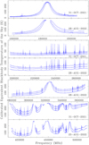 |
Fig. 2 Subset of the 56 fully calibrated and cleaned atmospheric scans used in this study to validate CIA absorption terms in the ATM radiative transfer model. The several curves in each panel correspond to observations at different air mass values for each date listed in Table 1. The air mass increases from lower to upper equivalent blackbody temperature curves. |
4 Observing runs and results
In order to conduct the necessary observing campaigns, we applied for APEX telescope time via a ‘calibration’ proposal in 2019, and again in 2022 for an extension of the same programme (105.2084.001). In total, we obtained around 40 hours of telescope time, which were divided into several observing sessions focussing on different atmospheric windows, seasons, times of day, and overall atmospheric conditions, in particular PWVCs.
The observational part of this study was affected by the global COVID-19 pandemic, which prevented some trips to the observatory that had been planned to conduct these highly non-standard observations on site. Nevertheless, the team managed to have a series of online meetings to refine the observing strategy after each run and to discuss different technical aspects of these observations and the progressing results. Normal operations were resumed in 2022, and J.R. Pardo was also able to travel to the telescope in August-September 2022 for scheduled observations.
We focussed our previous Pardo et al. (2022) paper on the observations conducted on December 6 2020 under very dry atmospheric conditions. It is time now to perform an overall analysis using all the data obtained in 11 different runs between October 21, 2020 and September 3, 2022. The first calibration of the December 6, 2020 data revealed calibration problems that took a long time to be solved. Many discussions were necessary to identify different issues and to try to implement satisfactory solutions. The main difference between using the telescope for atmospheric measurements and for astronomical observations is that in the first case we have to achieve an accurate absolute calibration using two reference loads, and in the second case we work in differential mode between the astronomical target and the sky around it. In addition, the strong signal from the atmosphere can cause baseline problems and we cannot subtract any baseline.
The final spectra used in this work are fully calibrated in absolute terms after all the above-mentioned solutions were implemented (see Sect. 3).
Within each observing date, spectra at different airmasses were recorded in order to check for consistency in the PWVC retrievals. However, two different strategies were followed for those skydips as several tunings are necessary to cover all frequencies reachable by one particular receiver.
In some cases, the tuning was done and the telescope moved to the different airmasses to collect data in all of them before moving to the next frequency tuning. This implies that quite a long time was necessary to complete the frequency coverage in one band for all the airmasses, giving enough time for the PWVC to change significantly. This is the case of the SEPIA660 skydip of five airmasses (1.0, 1.25, 1.5, 1.75, and 2.0) taken on December 6, 2020. It took 3 hours and 10 minutes to complete it. The ATM model gives an average PWVC from fitting those data of ~0.34 mm, in good agreement with the average value retrieved from the water vapour radiometer (WVR). However, according also to the WVR data there was an PWVC increase from the beginning to the end of those observations of about 10% of the average value. Introducing this slope in the inputs of ATM significantly reduces the fit residual, giving support to the analysis (see Fig. 3).
In later cases, we adjusted the observing set-up to keep the environmental conditions as constant as possible for a given airmass. The elevation was kept constant, passing through all frequency tunings before moving to a different elevation or air-mass. The number of airmasses was reduced to three (1.0, 1.5, and 2.0). In those cases, a complete frequency coverage of a particular band for a given elevation takes a shorter time, reducing the chances of strong PWVC changes. However, the PWVC evolution can show up from one airmass to another.
Not all the observing runs provided useful results due to technical problems, errors in the observing procedure due to its highly non-standard nature, or too-large fluctuations in the atmospheric conditions. A total of 56 useful spectra providing a reasonably good coverage of frequencies and atmospheric conditions could be used for the goals of this study. The most relevant information about these observing runs is summarised in Table 1, such as the receiver used, valid frequency range, air-masses, date, UT range, and average atmospheric P/T conditions from the weather station. Most of the observations were achieved by keeping constant the airmass and doing all the frequency tunings and scans before moving the telescope to a different elevation. A few observations, however, were done by keeping the same frequency tuning and moving the telescope to take a scan for each elevation before tuning again. Since the atmospheric conditions evolve during the observations, neither observing mode can provide a view of a complete skydip under constant conditions, but the overall results provide a good consistency between the data and the model (see Sects. 5 and 6).
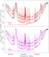 |
Fig. 3 ATM model fit to the skydip data obtained with APEX on December 6 2020 using the SEPIA660 receiver. Only three airmasses (1.0, 1.5, and 2.0) are plotted here for clarity (scans at 1.25 and 1.75 air-mass were also taken). Since the observations took over three hours to complete, the PWVC changed significantly and it was necessary to fit an average value plus a slope for it, with a great improvement in the agreement. |
5 Analysis
The main goal of this atmospheric study with APEX is to check the accuracy of the current ATM model at all frequencies covered by the observations presented in the previous section. The model relies upon a description of the different opacity terms (lines + CIA). Additionally, the model uses a priori vertical profiles of pressure, temperature, and molecular abundances based on simple assumptions from the available data provided by the weather station and the WVR. Specifically, we focus in this paper on the validation of the CIA absorption terms (in units m−1) described in the model as follows Pardo et al. (2001b) as a function of the frequency, ν, in gigahertz, the local temperature, T, in Kelvin, the water partial pressure  in millibars, and the dry partial pressure (
 in millibars):
![Mathematical equation: $\matrix{ {CI{A_{\left( {{O_2} - {H_2}O} \right) + \left( {{N_2} - {H_2}O} \right)}} & & & & & } \cr {\quad = 0.0315 \cdot {{\left( {{v \over {225}}} \right)}^2} \cdot \left[ {{{{P_{{H_2}O}}} \over {1013}} \cdot {{{P_{dry}}} \over {1013}}} \right] \cdot {{\left( {{{300} \over T}} \right)}^3}} \cr } $](/articles/aa/full_html/2025/01/aa52159-24/aa52159-24-eq3.png) (1)
(1)
 (2)
(2)
It is necessary to add another dry term (3) due to the non-resonant relaxation (Debye) spectrum of O2 (Sect. 2.2 of Liebe et al. 1993). For the frequency range, observation geometry, and atmospheric conditions explored in this work, this extra term produces an integrated contribution to the total zenith opacity of 0.0029 (constant with frequency) that is slightly less than 6% of the value produced by the dry CIA according to Eq. (2) at 650 GHz. However, the importance of this constant term with respect to the ∝ ν2 dry CIA obviously increases as the frequency decreases. In our analysis, both dry non-resonant terms are included or removed simultaneously.
The integral of the (1) and (2)+(3) terms through the whole atmospheric path results in the red and pink curves, respectively, of Fig. 1, which are examined in the rest of this paper, using the 56 SEPIA and nFLASH APEX atmospheric spectra summarised in Table 1 and the scans simultaneously performed the APEX WVR. This instrument provides measurements of the atmospheric brightness temperature of the 183 GHz water line in six defined band-passes to spectrally characterise the emission symmetrically from the centre of the water line (183.310 GHz) with a given bandwidth.
From the closest to the H2O line centre outwards, the offsets of the WVR double sideband channels are (in gigahertz): ±0.6, ±1.5, ±2.5, ±3.5, ±5.0, and ±7.5. Their bandwidths, respectively, are (also in gigahertz): 0.2, 0.2, 0.2, 0.2, 0.4, and 0.5.
Once the spectral data were taken, an atmospheric radiative transfer model (ATM) was used to fit the observations and estimate the PWVC. The key point here is that the atmospheric opacity, and therefore the brightness temperature, are both largely dominated by the 183 GHz water vapour line so that the derived PWVC from the WVR channels would barely reflect other aspects of the model such as minor gases, CIA, or far wings of other H2O lines (see Fig. 1). The percentage of the total opacity in the central three WVR channels (within ± 2.6 GHz of the line centre) that can be attributed to the water line exceeds 95% for 1 mm PWVC and the dry opacity represents less than 1.5%. However, PWVC retrievals from the whole set of frequencies in the APEX spectra presented in this work are quite different as minor gases and CIA opacity are in general much more important in the large frequency ranges of our APEX atmospheric spectra. In general, water lines do not dominate the opacity at all frequencies. Therefore, a simple exercise comparing the PWVC derived from WVR data and from fitting the APEX spectra themselves would provide a very strong model validation tool, chiefly for CIA.
In order to perform the proposed validation, we smoothed the 56 spectra to a resolution of 9.7 MHz, large enough for the broad atmospheric H2O and O2 lines and still providing several tens of channels on narrower O3, N2O, CO, and other features. We fitted those spectra to retrieve PWVC under some simple assumptions:
Pressure and temperature at the ground were fixed to the average values provided by the weather station during the scan.
The tropospheric temperature lapse rate was fixed to – 5.6 K/km.
The tropospheric water vapour scale height was fixed to 2.5 km.
The stratospheric and mesospheric P/T profiles were fixed to the U.S. Standard Atmosphere (1976) values for a tropical atmosphere, eventually displaced to match the values in the tropopause reached with the above assumptions.
The ozone profile was fixed by hand to minimise residuals near its lines, but with no true fit.
Vertical distributions of other minor gases were left as in the U.S. Standard Atmosphere (1976) tropical atmosphere.
In a separate publication, finer fits for O3 and other gases will be performed. For now, a first fit has been carried out with the full opacity breakdown in the ATM model: H2O and dry atmospheric lines below 1 THz, including all relevant isotopologues and vibrationally excited states, dry and wet CIA, and far wings of supra-terahertz water vapour lines. Then other fits were carried out removing one or several of these opacity contributions.
Summary of 56 atmospheric spectra, from 11 different APEX observing runs, used in this work.
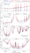 |
Fig. 4 Selection of spectra used in this study, showing the result of the best PWVC fit given by the ATM full model, and the effect on the atmospheric brightness temperature when the same fitted PWVC is used but different opacity contributions are removed from the calculations. |
6 Discussion
In recent years, a number of publications have addressed the question of the non-resonant foreign wet and dry CIA in the atmosphere from theoretical calculations or laboratory experiments under well-controlled conditions (Boissoles et al. 2003, Podobedov et al. 2008, Tretyakov at al. 2015, Serov at al. 2020). Our observations, of course, are under less controlled conditions and we detect the radiation after its propagation through the whole atmosphere to our detectors. Therefore, we cannot address the fine details given in the above-cited publications. However, the description of these opacity terms in ATM for the conditions of millimetre and sub-millimetre ground-based observatories can be validated with our data, even with the experimental data scatter that we can expect in this 3 year study. Even so, this validation is a big step forwards in the state-of-the-art of atmospheric models used by the observatories.
Following the procedure explained in the previous section, we have plotted, for each one of the 56 APEX spectra, PWVC fit results against the temporal average of the WVR-based PWVC. Although experimental scatter should be expected, if the model has a correct CIA description, an alignment around the diagonal line should be found. On the contrary, a misalignment should appear if the full model is inconsistent, or if different terms of the correct model are removed. Figure 5 shows the results of this exercise. The top left panel corresponding to the full ATM model shows a relatively good agreement for the whole PWVC range of ~0.35 mm to 3.5 mm, or one order of magnitude. An inset provides a closer look into the 0.3–0.8 mm PWVC range. There are three dark blue dots around 1.0–1.3 mm that appear a bit off the diagonal line. They correspond to a three airmass skydip taken with nFLASH230 on October 31 2021. Since the nFLASH230 band does not include any strong water line, it is the most sensitive to possible calibration issues. Nevertheless, we have decided to keep those spectra in the analysis as they provide significant information on all other panels.
The disagreement between the dots in the top left panel of Fig. 5 and the perfect diagonal line is only 6.25%, a value that seems compatible with the expected experimental scatter. There are three blue data points (NFLASH230 receiver) around 1.2–1.4 mm PWVC that show the largest deviation from the diagonal line. Due to the very low atmospheric opacity in the frequency range of the NFLASH230 receiver, deviations like this can somehow be expected as the PWVC retrieval from that frequency range is more uncertain than at higher frequencies. However, due to the large number of other data points, the conclusions do not change much. In fact, other blue data points in this panel at PWVC > 2.8 mm, for which the PWVC retrieval from the NFLASH230 spectra is less uncertain, show much less deviation from the diagonal.
The top right panel of Fig. 5 shows that, as was expected, the foreign wet collision-induced absorption due to both O2–H2O and N2–H2O collision mechanisms is a relevant element in the model as its removal produces a large disagreement in that panel (+55.79% average difference of the vertical axis values with respect to the horizontal axis ones, retrieved from the WVR, taken as a reference as explained in Sect. 5). The largest disagreement is in the dark blue dots that correspond to nFLASH230 spectra in a frequency region where, as was said before, foreign wet CIA is the dominant opacity term. On top of that, there is a general trend of more disagreement for wetter situations, and this can be also seen in SEPIA180 or SEPIA345 because these spectra cover not only the strong 183 GHz or 325 GHz water lines, but a significant range of window frequencies where, in fact, foreign wet CIA opacity has a larger share of the total opacity.
In general, the dry CIA (N2–N2, N2–O2, O2–O2 collisions) is much more constant and weaker (except for very dry situations) than the wet CIA. Therefore, its effect is much more limited, as is shown by the plot in the bottom left panel where we have removed the dry CIA term from the model in addition to the foreign wet CIA. The overall difference from the diagonal line increases now to 63.10%. Finally, removing the far wings of H2O lines centred above 1 THz also adds to the disagreement (bottom right panel of Fig. 5), which increases to 89.60%.
These results are quite conclusive: the ATM model needs all the original opacity terms to provide consistent results at least for the atmospheric conditions corresponding to high and dry millimetre and sub-millimetre observatories, as was the case for Mauna Kea and now Chajnantor. Based on these results, we would not suggest any changes in the model that may affect broadband opacity terms.
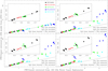 |
Fig. 5 PWVC provided by the WVR (average over the scan) vs the one derived from ATM fits of APEX spectra under various scenarios. The inset in each panel corresponds to a zoom-in of the area marked by the dotted box. The solid black line in each panel, and in the insets, marks the bisector or diagonal or equal PWVC values derived from the two methods. |
7 Summary and conclusions
We have studied the CIA terms in the atmospheric model ATM for the typical atmospheric conditions reigning on the Chajnantor Plateau with one order of magnitude range in the PWVC, using well-calibrated spectra covering full frequency ranges for five receivers from ~157 to 742 GHz. The analysis reveals that all CIA terms derived ~20–25 years earlier from atmospheric scans with the Caltech Submillimeter Observatory in Mauna Kea seem to be correct to the extent of the experimental scatter with APEX at Chajnantor, and should remain unchanged in the model. Further measurements are advised with the nFLASH230 receiver due to its special sensitivity to the CIA terms. Completing the study with more data beyond 752 GHz, into the next sub-millimetre window, and below ~170 GHz (including in higher PWVC conditions that can be used for astronomical observations at such frequencies), is also desirable. The results of this study strongly depend on a correct absolute calibration and, for that reason, a long time has been devoted to understanding and refining it as much as possible, resulting in a benefit for the APEX telescope.
Acknowledgements
This publication is based on data acquired between October 2020 and September 2022 with the Atacama Pathfinder EXperiment (APEX) under programme ID 105.2084 within the framework of an ESO/ALMA development study under contract CFP/ESO/19/25417/HNE. APEX is a collaboration between the Max-Planck-Institut für Radioastronomie, the European Southern Observatory, and the Onsala Space Observatory. JRP also thanks ESO for funding the implementation of ATM in the ALMA software under contract 14977/ESO/07/15694/YWE. Additional support has also been provided by EUMETSAT under contract EUM/20/4600002477. Part of this work was carried out at the Jet Propulsion Laboratory, California Institute of Technology, under a contract with NASA (80NM0018D0004).
References
- Belitsky V., Lapkin I., Fredrixon, M., et al. 2018, A&A, 612, A23 [NASA ADS] [CrossRef] [EDP Sciences] [Google Scholar]
- Boissoles, J., Boulet, C., Tipping, R. H., Brown, A., & Ma, Q. 2003, JQSRT, 82, 505 [NASA ADS] [CrossRef] [Google Scholar]
- Chamberlin, R. A., Martin, R., Martin, C. L., & Stark, A. A. 2003, SPIE Proc., 4855, 609 [NASA ADS] [CrossRef] [Google Scholar]
- Güsten, R., Nyman, L. Å., Schilke, P., et al. 2006, A&A, 454, L3 [Google Scholar]
- Hills, R. E., Webster, A. S., Alston, D. A., et al. 1978, Infrared Phys., 18, 819 [NASA ADS] [CrossRef] [Google Scholar]
- Ji, Y., Cheng-Hua, S., Shu-Ping, H., Ohishi, M., & Miyazawa, K. 2004, Chinese Astron. Astrophys., 28, 367 [CrossRef] [Google Scholar]
- Klein, B., Hochgürtel, S., Krämer, I., et al. 2012, A&A, 542, L3 [NASA ADS] [CrossRef] [EDP Sciences] [Google Scholar]
- Klein, U., Loiselet, M., Mason, G., Gonzalez, R., & Brandt, M. 2016, ESA’s Ice Cloud Imager on Metop Second Generation, EGU General Assembly Conference Abstracts, 17750 [Google Scholar]
- Liebe, H. J., Hufford, G. A., & Cotton, M. G. 1993, Proceedings of AGARD 52nd Specialists’ Meeting of the Electromagnetic Wave Propagation Panel, Palma de Mallorca (Spain) [Google Scholar]
- Meledin, D., Lapkin, I., Fredrikson, M., et al. 2022, A&A, 668, A2 [NASA ADS] [CrossRef] [EDP Sciences] [Google Scholar]
- Matsushita, S., Matsuo, H., Pardo, J. R., & Radford, S. 1999, PASJ, 51, 603 [NASA ADS] [CrossRef] [Google Scholar]
- Matsushita, S., Asada, K., Martin-Cocher, P. L. et al. 2017, PASP, 129, 025001 [NASA ADS] [CrossRef] [Google Scholar]
- Mlawer, E. J., Turner, D. D., Paine, S. N., et al., 2019, JGR Atmospheres 124, 8134 [NASA ADS] [CrossRef] [Google Scholar]
- Mlawer, E. J., Cady-Pereira, K. E., Mascio, J., & Gordon, I. E. 2023, JQSRT, 306, 108645 [NASA ADS] [CrossRef] [Google Scholar]
- Ningombam, S. S., Sethulakshmy, E. S., Jade, S., et al. 2020, J. Atmos. Sol.-Terrestr. Phys., 105404 [NASA ADS] [CrossRef] [Google Scholar]
- Paine, S., Blundell, R., Papa, D. C., Barrett, J. W., & Radford S. J. E. 2000, PASP, 112, 108 [CrossRef] [Google Scholar]
- Pardo, J. R., Serabyn, E., & Cernicharo, J. 2001a, JQSRT, 68, 419 [NASA ADS] [CrossRef] [Google Scholar]
- Pardo, J. R., Cernicharo, J., & Serabyn, E. 2001b, IEEE Trans. Antennas Propag., 49, 12 [Google Scholar]
- Pardo, J. R., Serabyn, E., Wiedner, M. C., & Cernicharo, J. 2005, JQSRT, 96, 537 [NASA ADS] [CrossRef] [Google Scholar]
- Pardo, J. R., de Breuck, C., Muders, D., et al. 2022, A&A, 664, A153 [NASA ADS] [CrossRef] [EDP Sciences] [Google Scholar]
- Podobedov, V. B., Plusquellic, D. F., Siegrist, K. E., et al. 2018, JQSRT, 109, 458 [Google Scholar]
- Serov, E. A., Balashov, A. A., Tretyakov, M. Yu., et al. 2020, JQSRT, 242 [Google Scholar]
- Shi, S. C., Paine, S., Yao, Q. J., et al. 2016, Nat. Astron., 1, 0001 [NASA ADS] [CrossRef] [Google Scholar]
- Tretyakov, M. Yu., Sysoev, A. A., Odintsova, T. A., & Kyuberis, A. A. 2015, Radiophys. Quant. Electron., 58, 262 [NASA ADS] [CrossRef] [Google Scholar]
- Tremblin, P., Schneider, N., Minier, V., Durand, G. Al., & Urban, J. 2012, A&A, 548, A65 [NASA ADS] [CrossRef] [EDP Sciences] [Google Scholar]
- Ulich, B. L. 1980, ApJ, 21, L21 [Google Scholar]
- Ulich, B. L., & Haas, R. W. 1976, ApJS, 30, 247 [Google Scholar]
- U.S. Standard Atmosphere 1976, U.S. Government Printing Office, Washington, D.C. [Google Scholar]
All Tables
Summary of 56 atmospheric spectra, from 11 different APEX observing runs, used in this work.
All Figures
|
Fig. 1 Reference ATM model for the APEX site, considering 555 hPa and 273 K as physical parameters at the ground, and 0.5 (dotted black and red lines), 1.0 (solid black and red lines), and 2.0 mm (dashed black and red lines) of the PWVC. Note that the H2O–H2O (self wet) CIA is in practice negligible in these very dry conditions (only the curve for 2.0 mm PWVC is shown in a dashed green colour as the curves for 1.0 and 0.5 mm PWVC are below the bottom Y limit of the plot). The frequency ranges covered by the SEPIA and nFLASH receivers used in this work are plotted for reference, as are ALMA bands 5–9. The central frequencies of the six double side-band channels of the APEX WVR, on both sides of the 183.31 GHz H2O line, are also plotted. The red and pink ClA curves are the ones under validation in this paper. Cyan (minor gases opacity), blue (O2 lines opacity) and pink (dry CIA opacity) curves remain unchanged for all PWVC values. |
| In the text | |
|
Fig. 2 Subset of the 56 fully calibrated and cleaned atmospheric scans used in this study to validate CIA absorption terms in the ATM radiative transfer model. The several curves in each panel correspond to observations at different air mass values for each date listed in Table 1. The air mass increases from lower to upper equivalent blackbody temperature curves. |
| In the text | |
|
Fig. 3 ATM model fit to the skydip data obtained with APEX on December 6 2020 using the SEPIA660 receiver. Only three airmasses (1.0, 1.5, and 2.0) are plotted here for clarity (scans at 1.25 and 1.75 air-mass were also taken). Since the observations took over three hours to complete, the PWVC changed significantly and it was necessary to fit an average value plus a slope for it, with a great improvement in the agreement. |
| In the text | |
|
Fig. 4 Selection of spectra used in this study, showing the result of the best PWVC fit given by the ATM full model, and the effect on the atmospheric brightness temperature when the same fitted PWVC is used but different opacity contributions are removed from the calculations. |
| In the text | |
|
Fig. 5 PWVC provided by the WVR (average over the scan) vs the one derived from ATM fits of APEX spectra under various scenarios. The inset in each panel corresponds to a zoom-in of the area marked by the dotted box. The solid black line in each panel, and in the insets, marks the bisector or diagonal or equal PWVC values derived from the two methods. |
| In the text | |
Current usage metrics show cumulative count of Article Views (full-text article views including HTML views, PDF and ePub downloads, according to the available data) and Abstracts Views on Vision4Press platform.
Data correspond to usage on the plateform after 2015. The current usage metrics is available 48-96 hours after online publication and is updated daily on week days.
Initial download of the metrics may take a while.