| Issue |
A&A
Volume 693, January 2025
Solar Orbiter First Results (Nominal Mission Phase)
|
|
|---|---|---|
| Article Number | A185 | |
| Number of page(s) | 10 | |
| Section | The Sun and the Heliosphere | |
| DOI | https://doi.org/10.1051/0004-6361/202452030 | |
| Published online | 15 January 2025 | |
Effects of cold electron emissions on thermal plasma measurements on board Solar Orbiter spacecraft
1
Institute of Atmospheric Physics of the Czech Academy of Sciences, Boční II 1a/1401, 14100 Prague, Czech Republic
2
Astronomical Institute of the Czech Academy of Sciences, Boční II 1a/1401, 14100 Prague, Czech Republic
3
Department of Space and Climate Physics, Mullard Space Science Laboratory, University College London, Dorking, Surrey RH5 6NT, UK
4
Swedish Institute of Space Physics (IRF), Uppsala 75121, Sweden
5
Sothwest Research Institute, 6220 Culebra Road, San Antonio TX 78238-5166, USA
6
LESIA, Observatoire de Paris, Université PSL, CNRS, Sorbonne Université, Université de Paris, 5 Place Jules Janssen, 92195 Meudon, France
⋆ Corresponding author; stverak@ufa.cas.cz
Received:
28
August
2024
Accepted:
18
November
2024
Aims. Emissions of photo and secondary electrons influence thermal electron measurements on board spacecraft, typically below a threshold determined by the spacecraft’s potential. We aim to examine and quantify this contamination of the observed low-energy electron fluxes. We seek to provide effective constraints for the correction methods used to accurately estimate unperturbed solar wind plasma parameters in the context of the Solar Orbiter mission.
Methods. We performed a long-term statistical analysis of electron velocity distribution functions acquired by the Electron Analyser System experiment, which is part of the Solar Orbiter’s Solar Wind Analyser suite of instruments. We employed analytical fits of time-averaged phase space density spectra to identify the energy break separating ambient solar wind electron populations from cold electron populations emitted by the spacecraft body. We analysed correlations between the observed energy break and the spacecraft potential, as well as other relevant plasma properties.
Results. Our analysis indicates that in contrast to other space missions, emitted electrons from the spacecraft are detected even above the spacecraft potential energy. The derived energy break is found to be uncorrelated with the measured spacecraft potential, but it is correlated strongly with the ambient electron temperature. We attribute this behaviour to the Solar Orbiter’s geometric configuration, which can result in the detection of electrons emitted from spacecraft surfaces that are located far from the instrument’s detector. We derived a theoretical expression for the energy break, assuming Maxwellian distribution functions for both the ambient and spacecraft electrons. This provides an effective constraint for the observed contamination by spacecraft electrons.
Key words: instrumentation: detectors / methods: data analysis / solar wind
© The Authors 2025
 Open Access article, published by EDP Sciences, under the terms of the Creative Commons Attribution License (https://creativecommons.org/licenses/by/4.0), which permits unrestricted use, distribution, and reproduction in any medium, provided the original work is properly cited.
This article is published in open access under the Subscribe to Open model. Subscribe to A&A to support open access publication.
1. Introduction
Electrons in the solar wind are mostly observed to be far from local thermal equilibrium (Montgomery et al. 1968; Feldman et al. 1975; Rosenbauer et al. 1977; Pilipp et al. 1987; Maksimovic et al. 2005; Štverák et al. 2009) and their radial evolution exhibits significant deviations from simple adiabatic predictions (e.g. Ogilvie & Scudder 1978; Feldman et al. 1979; Pilipp et al. 1990; Scime et al. 1994a; Issautier et al. 1998; Maksimovic et al. 2000; Štverák et al. 2015). The classical fluid approach is not fully applicable because many processes governing the electron behaviour are kinetic in nature (Marsch 2006; Verscharen et al. 2019, 2022). Precise in situ measurements of electron velocity distribution functions (VDFs) are needed to properly analyse and test models and their predictions on the basis of kinetic (Maxwell-Boltzmann) theory.
The field of space plasma diagnostics, however, brings up a number of not only scientific but first also instrumental and data processing challenges. Experiments for in situ plasma measurements, typically represented by charged particle electrostatic energy analysers (e.g. Hutchinson 2002), have to deal with limited hardware performance, consequently leading to considerable constraints on the instrumental resolution, signal-to-noise ratio, and related in-flight or on-ground calibration issues. Even assuming an ideal perfect plasma detector, appropriate methods must be applied to derive correct parameters of a model plasma environment from acquired VDF samples (Song et al. 1997; Génot & Schwartz 2004; Geach et al. 2005; Lavraud & Larson 2016). For a real space plasma instrument, the situation becomes even more difficult as the observed plasma environment can be significantly disturbed by the presence of the spacecraft structure and/or the plasma detector itself. Following the classical theory of Langmuir & Blodgett (1924) and Mott-Smith & Langmuir (1926), any spacecraft immersed into a plasma environment immediately starts to absorb fluxes of ambient electrons and ions, while concurrent fluxes of photoelectrons, secondary electrons, or backscattered electrons are, in turn, emitted from the surface of the spacecraft body itself. Currents induced by both the collected and emitted fluxes result in electrical charging of the spacecraft structure creating a non-zero potential with respect to the ambient plasma background. All fluxes come into a balance to meet the zero net current condition (preventing an infinite charging) at a specific electric potential, ΦSC, known as the spacecraft floating potential. The value of the spacecraft potential strongly depends on the local ambient plasma properties, solar radiation, and specific design aspects of the spacecraft itself (Grard 1973; Berry Garrett 1981; Whipple 1981; Pedersen 1995; Scudder et al. 2000). Assuming a fully conductive spacecraft, the potential is set rather rapidly according to the characteristic local electron time scales. For a typical range of observed solar wind parameters at 1 AU, the charged particle fluxes are mostly dominated by photoelectron emissions, resulting in a positive spacecraft potential of up to about 15 V in the case of very tenuous and cold plasma states. The spacecraft potential may possibly become slightly negative due to increased ambient electron fluxes for events with extremely high plasma densities and temperatures (e.g. Salem et al. 2001).
For ambient electrons, a positive (and thus attractive) potential ΦSC > 0 accelerates negative charges towards the spacecraft and increases their kinetic energy by eΦSC when reaching the spacecraft surface or any instrument aperture. The spacecraft potential effect differs for local electron populations emitted from the spacecraft surface. Electrons emitted at energies above eΦSC can escape the potential barrier and leave the spacecraft to the ambient environment, while electrons with initial energies below eΦSC are trapped by the potential and are forced to fall back to the surface, having equal initial and impacting kinetic energies. From all the emitted electrons, only those that escape contribute to the spacecraft net charging. For an ideal plasma detector, this means that all ambient electrons are detected and observed in the energy spectrum above eΦSC, while particle fluxes observed below eΦSC are collected due to the trapped electrons emitted from the spacecraft surface. For on ground data processing, like for example electron moments calculation from VDFs, the measured spectra below eΦSC, contaminated by spacecraft electron fluxes, have to be excluded from the analysis.
In the simplified scalar spacecraft potential approach, the attracting potential affects only the radial component of particle velocities. All measured particle energies are then corrected by subtracting eΦSC to get initial particle energies in the ambient plasma (e.g. Génot & Schwartz 2004; Lavraud & Larson 2016). Such a correction equally removes all measured spacecraft emitted electrons trapped below the eΦSC threshold. However, the electric field induced by spacecraft charging not only changes the particle kinetic energy but may also affect the particle velocity direction. In plasma experiments, the measured velocity vector of an impacting particle therefore does not necessarily correspond to its initial velocity direction in the unperturbed ambient environment. Changes in particle trajectories become significant namely for plasma environments with a large Debye length, compared to the characteristic dimensions of the spacecraft, or of the instrument itself, and for particles with initial energies comparable to or below eΦSC. The scalar approach may be further invalidated by the possible asymmetries of electric potential fields resulting from complex spacecraft body geometries or differential charging effects. To correct the measurements for these particle trajectory effects as well, the appropriate enhanced models and methods have to be applied within on ground data processing (e.g. Scime et al. 1994b; Bouhram et al. 2002; Hamelin et al. 2002; Pulupa et al. 2014) to properly derive any directional quantities. These include the bulk velocity, heat flux, or other specific directional VDF moments defined with respect to the local magnetic field direction.
Precise knowledge of the spacecraft potential is crucial for any space plasma experiment to correctly interpret raw measurements. Most modern plasma missions are therefore equipped with electric probes or antennas designed to directly estimate the spacecraft potential value by measuring the voltage of a biased probe (locally grounded to plasma) with respect to the spacecraft ground (Pedersen 1995; Scudder et al. 2000; Pedersen et al. 2008; Lindqvist et al. 2016; Khotyaintsev et al. 2021). Other indirect methods have to be used for missions with limited instrumentation. As a common alternative, the spacecraft potential can often be indirectly estimated by cross-calibrating the plasma parameters derived from electron VDF measurements with other independent plasma instruments and diagnostic techniques (e.g. Salem et al. 2001; Štverák et al. 2009; Salem et al. 2023). When relying only on measured VDFs, the break in the spectrum between the ambient and spacecraft emitted electron populations is amply recognised as another possible proxy estimate of the spacecraft potential value (Phillips et al. 1993; Lewis et al. 2008; Lavraud & Larson 2016; Wilson et al. 2023).
In the case of the Solar Orbiter mission, a preliminary work on correcting raw electron measurements and deriving ambient electron bulk properties was performed by Nicolaou et al. (2021). Therein, the authors developed and validated two methods for calculating the moments of a model VDF, as seen by an ideal detector; first, they used a direct numerical integration of the measured VDF and then fitt a model VDF to the measured data. The two methods were consequently applied to a limited dataset of real in situ measurements. The derived electron density was shown to have a fair qualitative agreement with relevant observations from other on board measurements, but with an offset in absolute values, possibly indicating a need for improved cross calibrations of the different experiments. The effect of the spacecraft potential was not considered by Nicolaou et al. (2021) and the artificial fluxes from spacecraft emitted electrons were removed by applying a fixed energy cut-off, based solely on an overall visual inspection of the relevant dataset.
On board Solar Orbiter, a single point estimate of the spacecraft potential value is provided by a DC voltage technique (Khotyaintsev et al. 2021), possibly applicable to the simple scalar approach method. However, preliminary numerical simulations of Guillemant et al. (2012), Guillemant (2014), Guillemant et al. (2017) have shown a rather complex structure of the electric field surrounding the spacecraft body, with variable particle trajectory effects in different instrument look directions. A question also arises if and how the measured spacecraft potential value is relevant and valid for electron VDF measurements, performed in the case of Solar Orbiter mission rather far away from the main spacecraft structure at the tip of the deployable instrument boom. Another concern is whether, in practice, the measured spacecraft potential value is still applicable for removing the artificial fluxes of spacecraft emitted electrons and for correcting the energy levels (and velocity directions) of collected ambient electrons.
In this paper, we aim to investigate the first of the two problems, namely, to test and analyse if and how the measured spacecraft potential is linked to the energy break observed in measured electron VDF spectra between the spacecraft and ambient electron populations. The second issue of ΦSC effects on the energies and velocity directions of ambient electron fluxes will be part of a follow-up study. We first developed and implemented a method for the separation of ambient and spacecraft emitted electrons in measured VDF spectra to localise the energy break between the two populations. We applied the method to a statistically significant dataset of real in situ observations performed by Solar Orbiter. The dataset and the method itself are described in Sect. 2. Subsequently, we analysed resulting correlations of the energy break values with the measured spacecraft potential values and other relevant plasma properties. Our main results are presented in Sect. 3 and further discussed in Sect. 4. Finally, we assessed possible applications of our findings in enhanced VDF correction methods as summarised in Sect. 5.
2. Data analysis
2.1. Dataset
We performed the present study using in situ solar wind observations acquired by Solar Orbiter mission (Müller et al. 2020; Zouganelis et al. 2020) in the full year of 2021. All data used in our study are available via the public Solar Orbiter archive1 (SOAR) provided by the European Space Agency (ESA). In particular, we analysed the electron velocity distribution functions measured by the Electron Analyser System (EAS), which is part of the Solar Wind Analyser (SWA) suite of instruments (Owen et al. 2020). Figure 1 shows the coverage of the radial distance from the Sun for the year 2021, along the spacecraft trajectory, corresponding to more than one full orbit around the Sun, with its perihelion and aphelion at about 0.5 and 1 AU, respectively. The figure also shows the data availability from the SWA-EAS experiment.
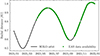 |
Fig. 1. Radial coverage (black line) and SWA-EAS data availability (green dots) shown as a function of time along the Solar Orbiter trajectory in the year 2021. |
The SWA-EAS instrument is designed to measure full 3D electron VDFs by the use of two top-hat electrostatic analysers, EAS1 and EAS2, mounted on the main spacecraft boom and directed anti-sunwards into the shadow behind the spacecraft body. Both EAS sensors are capable of covering the full 360° of azimuth in 32 equal steps and the electrostatic deflection system provides elevation coverage of ±45° in 16 non-monotonic steps, with the angular resolution being driven by the instrument’s design and geometry. The main axes of the two top-hat sensors are separated by 90° from each other, so that the combined field of view (FOV) of the two detectors covers almost full 4π of the sky, although a small part of the FOV is blocked by the mechanical structure of the spacecraft and the instrument itself. The measured energy range starts at less than 1 eV and goes up to 5 keV in 64 logarithmically spaced steps, resulting in an almost constant energy bandwidth of ΔE/E ≈ 13%. Both SWA-EAS sensors were designed to sample the full set of angular and energy steps (16 × 32 × 64) every one second. The acquired samples were further processed for data downlink, using several data acquisition modes implemented for nominal SWA-EAS observations. For our analysis, we used the on ground processed phase space densities (PSD), referenced as Level 2 Normal Mode 3D (NM3D) data products in SOAR, with a time resolution of either 10 or 100 seconds per VDF sample.
In addition to electron VDFs measured by SWA-EAS, we used spacecraft potential values measured on board Solar Orbiter by the Radio and Plasma Waves (RPW) experiment (Maksimovic et al. 2020). The RPW instrument is primarily designed to measure local magnetic and electric fields and their fluctuations as electromagnetic wave spectra by using a three-axis search coil magnetometer and a set of three electric monopole antennas. In addition, by measuring and combining DC voltages of the three antennas with respect to the spacecraft body, the RPW experiment is also capable of providing reliable estimates of the spacecraft potential (Khotyaintsev et al. 2021; Steinvall et al. 2021; Maksimovic et al. 2021). The DC voltage on all RPW antennas is continuously measured with a sampling frequency of either 16 or 256 samples per second, which fully allowed us to match the time stamps of RPW data samples with those of the NM3D samples from the SWA-EAS experiment, measured with a much lower cadence. Spacecraft potential values are available in SOAR as the RPW Level 3 BIAS SCPOT data products. Additionally, we included to the dataset solar wind proton densities and bulk speeds, derived as on-ground moments of the ion 3D VDFs; these have been acquired by the Proton and Alpha Sensor (PAS) as another part of the SWA experiment, as reported in Owen et al. (2020). The on ground PAS proton moments are available as Level 2 GRND MOM data products in SOAR at temporal cadences ranging from 4 s to about 0.1 s. The PAS data products were used in the present study solely to characterise the general statistical properties of the dataset itself.
The SWA-EAS dataset from 2021 contains over one million EAS NM3D PSD samples; however, for our analysis, we time-averaged every 100 consecutive samples, so that the number of samples in the final dataset was reduced by this factor down to roughly eleven thousand. For a time resolution of 10 s, the sample window (of 100) corresponds to a time interval of approximately 17 minutes of measurements. Time averaging was applied to reduce the noise level and improve the statistical quality of individual data samples, as the raw SWA-EAS measurements often suffer from low count numbers. For typical solar wind densities of about 10 cm−3 at 1 AU, angular bins in the 3D VDFs with one or even zero count level are often observed across the whole instrument energy range due to a rather short acquisition time intervals required to scan the full set of angles and energies within one second of data acquisition. In the case of RPW and PAS data products, the samples were first selected to match the EAS time stamps and were consequently averaged in the same manner as the EAS data samples.
The basic statistical properties of the final reduced dataset are summarised as histograms in Fig. 2. The sample count rates are distributed fairly equally across the observed radial range (see Fig. 2a). The spacecraft potential is mostly positive, in agreements with theoretical predictions for solar wind plasma conditions, reaching up to about 12 V with a most probable value at about 6 V as shown in Fig. 2b. The histograms in Fig. 2c and Fig. 2d give the solar wind proton density, with peak values seen at approximately 10 cm−3, and the proton bulk speed, ranging mostly between 300–400 km/s. The dataset can be considered as statistically representative of typical (slow) solar wind conditions over the given radial range.
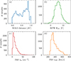 |
Fig. 2. Statistical properties of the dataset used in the present study. Histograms show (a) number of time-averaged data samples for the radial distance from the Sun; (b) spacecraft potential as derived from RPW measurements; (c) solar wind proton densities; and (d) solar wind proton bulk speeds received from PAS on ground moments. |
2.2. Methods
We have aimed to determine the expected break between cold spacecraft emitted electrons and thermal ambient (solar wind) electrons in the energy spectrum of the measured phase space density. Our motivation was to derive the characteristic properties of this energy break and confirm its expected correlation to the spacecraft potential value. We first demonstrated the expected properties of the energy break by constructing a model measurement as acquired by a virtual ideal EAS sensor. For simplicity, we considered the phase space density of ambient solar wind electrons in the plasma rest frame (PRF) to take the form of an isotropic Maxwellian distribution of particle velocities,
Here, ne, SW and Te, SW are the solar wind electron density and temperature, respectively, while me is the electron mass, vPRF is the velocity vector in the phase space given in the plasma rest frame, and k is the Boltzmann constant. In the spacecraft reference frame (SRF), the electron distribution as observed by a detector is further modified as the plasma drifts with respect to the probe. For a relative drift speed, ud, given as

where uSW and uSC are the solar wind bulk velocity and the spacecraft velocity vectors, respectively, both given in any common inertial reference frame with respect to the plasma and spacecraft reference frames, the particle velocity as seen by the spacecraft is given as
Following Liouville’s theorem, the phase space density in the spacecraft reference frame is given by

For our model, we further considered the simplified scalar spacecraft potential approach, where only the radial component of the particle velocity along its trajectory towards the detector is affected by the spacecraft potential. When a particle sensor is detecting electrons with a velocity vector, vΦSC, SRF, on a spacecraft positively charged to an electrostatic potential of ΦSC > 0, the initial electron velocity, vSRF, in the unperturbed spacecraft reference frame in this case is given as
where only the particle velocities with me|vΦSC|2/2 > eΦSC correspond to real ambient electron trajectories.
We note that for a theoretical case of a spacecraft moving with the plasma (i.e. ud = 0), the measured VDF after substituting Eq. (5) into Eq. (4) becomes

showing that by inserting a positive potential, ΦSC, into a plasma, the electron density is locally increased by the Boltzmann factor as
Using Eq. (1–5), the phase space density (as seen by an ideal EAS detector) can be derived in four steps. We let Ei be the kinetic energy, ϕj the azimuth, and θk the elevation of the instrument’s look direction for incoming electrons. We start (i) by applying the scalar approach for the spacecraft potential correction so that the kinetic energy, Ei, measured by the detector is simply converted to the true energy value, Ei, SRF, in the spacecraft reference frame. Specifically, we removed the acceleration effect of the positive spacecraft potential, ΦSC, as

(ii) next, we compute the particle velocity in SRF as

where rϕj, θk is the unit vector corresponding to the given look direction of the instrument defined by ϕj and θk. The negative sign in Eq. (9) is due to the fact that a particle entering the aperture from a given look direction must simply have an opposite velocity vector; (iii) finally, we transform the vijk, SRF to vijk, PRF by use of Eq. (3); and (iv) we compute the phase space density fijk, as seen by an ideal EAS sensor, directly from Eq. (1). For any Ei < eΦSC, we set fijk, SRF = 0.
Our model of the ideal EAS detector is similar to Nicolaou et al. (2021), except that we added the scalar effect of the spacecraft potential, as given by Eq. (8). We note here again that by considering the scalar correction for the spacecraft potential effect, we neglected possible changes in transversal velocity components that become of higher importance for asymmetric electric fields around the spacecraft and mostly for particle energies comparable or lower to eΦSC, knowing that the effect can be still possibly observed even at energies of several hundreds of eV (cf. Barrie et al. 2019).
The model velocity distribution function as seen by (16 × 32) angular bins of an ideal EAS sensor is shown in Fig. 3a as a function of the measured EAS energy levels. The black solid line corresponds to the ambient electron distribution fe, SW in the plasma rest frame given by Eq. (1) and the red dots show the distribution measured within all the individual angular bins of the ideal EAS detector in the reference frame of the spacecraft. The variation in the measured distribution at a given energy step is caused by the drift of the plasma with respect to the spacecraft (so that the look directions facing the solar wind stream show for a given energy a different part of the velocity phase space compared to those in the wake).
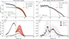 |
Fig. 3. Comparison between the model and measured data for an ideal Electron Analyser System (EAS) sensor. (a) The model phase space density as a function of energy. The contribution of the ambient solar wind electrons in the plasma reference frame (PRF) is shown as the black solid line. The red dots display the ambient electron distribution as seen by the individual FOV bins of an ideal EAS detector in the spacecraft reference frame (SRF). The contribution of the spacecraft emitted electrons trapped by the spacecraft potential (escaping away from the detector) is shown by the blue (green) dots. Black empty circles display the modelled EAS response averaged for each energy over all FOV directions of the instrument. The yellow line display the contribution of the ambient electron distribution modified by the spacecraft potential energy (denoted by the black dotted line). Panel b translates the results of panel a into differential energy fluxes. (c) Real EAS data samples in phase space densities (grey dots) in a format similar to panel a. The fitted contributions of the ambient, spacecraft, and all electrons as a function of energy. plotted with red, blue, and black dashed lines, respectively. Panel d recast the results of panel c in differential energy fluxes. For further reference we show in panel d the big blue, orange, and red circles the estimated peak differential energy flux of the spacecraft electrons Epeak, SC (big blue circle), the position of the break Ebreak (big orange circle), and the estimated peak of the differential energy flux of the solar wind electrons Epeak, SW (big red circle). |
For spacecraft-emitted electrons we assumed again for simplicity a Maxwellian distribution, as in Eq. (1), equal to

with a typically lower temperature of Te, SC < Te, SW and higher density, ne, SC > ne, SW, as compared to the thermally ambient electrons. For the model spacecraft electron measurements by the ideal EAS detector, we have two differences, compared to the model of ambient solar wind electrons. As they are emitted from the surface, these electrons are considered to have zero drift (on average) with respect to the spacecraft. Furthermore, for a positive spacecraft potential all electrons with an initial kinetic energy below eΦSC are attracted back to the surface and, thus, measured by the detector, while all other electrons emitted with energies above eΦSC are free to escape away from the instrument. Therefore, they do not contribute to the measured particle flux. In Fig. 3a, we plot the distributions of trapped spacecraft electrons and escaping spacecraft electrons with the blue and green dots, respectively.
For the density and temperature ratios of spacecraft to ambient electron population, typically observed at 1 AU in the solar wind, the full model VDF, shows a distinct break in the spectrum at energy eΦSC corresponding to the spacecraft potential as indicated in Fig. 3a by the black dotted line. Below this energy break, the measured model VDF is attributed to spacecraft-emitted electrons, while above the energy break, the measurements are not anyhow contaminated by spacecraft electrons and correspond purely to ambient electrons accelerated by the effect of the positive ΦSC.
The spacecraft and ambient electron populations and also the energy break are better distinguished when plotting the model measurements in terms of the differential energy flux (DEF), as shown in Fig. 3b, defined as
For our data analysis of real in situ EAS samples, we did not directly use the full measured 3D VDF f(Ei, ϕj, θk). Instead, we used the reduced 1D spectra fFOV(Ei) averaged over all instrument azimuths ϕj and elevations θk of the full detector’s FOV, so that
where ΔΩj, k is the surface on a unit sphere, corresponding to the solid angle of the angular bin for the given azimuth and elevation (ϕj, θk). Corrective effects of averaged PSD spectra for low count rates are described, for example, by Nicolaou et al. (2020). To a certain extent, FOV averaging can also mask the effect of plasma drift due to the solar wind bulk speed and spacecraft velocity. In Fig. 3, the averaged spectrum fFOV is plotted with black circles, whereas the yellow line represents the ambient electron distribution, fSW, Φ, modified in the plasma rest frame by the spacecraft potential, as given by Eq. (6). In the energy range above the spacecraft potential the FOV averaged PSD spectrum is reasonably close to the model given by Eq. (6), although the fFOV spectrum tends to slightly overestimate the real electron temperature due to the plasma drift (Nicolaou & Livadiotis 2016). Nevertheless, the definition of fFOV clearly does not affect the location of the energy break at eΦSC and, therefore, has no negative effect on our analysis.
The ideal model response of the sensor is compared to a real measured (time-averaged) data sample from SWA-EAS measurements, as shown in Fig. 3c,d. In that figure, we also illustrate the method used to separate the ambient and spacecraft electron fluxes. We identified the energy break between spacecraft and ambient electrons, together with two other relevant energy values in several consecutive steps: (i) we first computed fFOV from the 3D EAS VDF data as given by Eq. (12); (ii) fit the spectrum in a fixed energy range of 15–60 eV to get the measured VDF of spacecraft electrons. The minimum energy of 15 eV was set to be above the range of spacecraft potentials observed by RPW experiment (see Fig. 2b), while the upper limit was set to plausibly exclude the halo supra-thermal tails typically observed in the solar wind at higher energies (e.g., Štverák et al. 2009). For the fitting, we assumed the Maxwellian model for the thermal ambient electron population as given by Eq. (1) and employed standard linear regression to fit the logarithm of measured PSD as a function of energy; (iii) we derived the value of Epeak, SW as the energy corresponding to the maximum of the differential energy flux from the model fit of the thermal ambient electrons. This is shown by the red point in Fig. 3d; (iv) we then subtracted the initial fit of the thermal ambient electrons from the fFOV values; (v) we performed fit in the energy range from 3 eV to Epeak, SW. The upper fitting limit of Epeak, SW was set to safely exclude the supra-thermal part, where the Maxwellian model does not resolve the true ambient electron measurements. The low-energy cut-off at 3 eV was set as the performance of the EAS instrument drops at very low energies due to non-linearities of its high voltage power supply sub-system. The observed spectra at very low energies were typically found to deviate from the Maxwellian profile. To increase the robustness of the model for spacecraft electron VDFs, instead of linear regression as for ambient thermal electrons, we applied a polynomial regression of the second order to fit the logarithm of PSD as a function of the energy. Having both the ambient and spacecraft electron fits; and (vi) we further defined Epeak, SC in a similar manner to Epeak, SW, and, Ebreak as the energy of the local minimum of the total fit, in terms of the differential energy flux, in the energy range between Epeak, SC and Epeak, SW (see the blue and orange points in Fig. 3d, respectively). We note that the energy peak values, Epeak, * for the solar wind and spacecraft electrons were later used to provide a proxy estimate of the electron temperature as
knowing that for a Maxwellian distribution the differential energy flux reaches its maximum value at an energy of 2kTe, * (cf. Nicolaou & Livadiotis 2016, for a more general case of a drifting Kappa distribution).
3. Results
First, we plotted in Fig. 4 the value of ΦSC as a function of proton densities derived from PAS measurements to asses the quality of the spacecraft potential data product as derived from the RPW measurements. We demonstrated the spacecraft potential to decrease with increasing solar wind density. For lowest density values, the potential peaks at about 15 V, and the spacecraft potential becomes slightly negative for plasma densities above about 50 cm−3. In addition, we over-plotted the observed data with a theoretical formula for the spacecraft potential as given by Eq. (A7) from Salem et al. (2001) (see the black dashed line in Fig. 4). To calculate the single theoretical profile, we set a fixed radial distance of 0.8 AU, roughly corresponding to the mean radial distance in the observed radial range of our dataset. We further used characteristic plasma parameters for the given radial distance typically observed in the solar wind, namely, electron temperatures of 13 eV and 2 eV for the solar wind electrons and spacecraft photoelectrons, respectively.
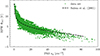 |
Fig. 4. Scatter plot of RPW spacecraft potential as a function of proton density derived from PAS measurements (green dots). Data are over-plotted by a theoretical profile (dashed line) computed using Eq. (A7) in Salem et al. (2001). |
The expected correlation between the spacecraft potential and the energy break in the VDF spectrum between the solar wind thermal electron population and cold electrons emitted from the spacecraft surface is plotted in Fig. 5. We show the derived specific energy values, Epeak, SC as blue and Ebreak as orange dots, from the complete dataset as a function of the spacecraft potential ΦSC as measured by the RPW experiment. The energy, Epeak, SC, corresponding to the peak value of the differential energy flux of detected spacecraft electrons, is rather constant with the spacecraft potential, having only small variations of values ranging roughly between 6 and 8 eV, thus corresponding to electron temperatures from about 3 to 4 eV according to Eq. (13). The theoretical correlation between the energy break and spacecraft potential, predicted by our model EAS response to simply be Ebreak = eΦSC, is plotted by the solid black line. The observed values of the energy break, Ebreak, are ranging from about 8 to 12 eV and are found to be nearly independent of the spacecraft potential value. The theoretical correlation of Ebreak to ΦSC is not confirmed by our results and Ebreak values are mostly found above the value of measured spacecraft potential.
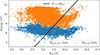 |
Fig. 5. Peak energy for the differential energy flux of spacecraft electrons Epeak, SC (blue dots) and energy for the spectrum break between spacecraft and ambient plasma electrons Ebreak (orange dots) is plotted as a function of the RPW spacecraft potential ΦSC. The black line shows the axis E = eΦSC corresponding to the expected correlation between Ebreak and ΦSC. |
4. Discussion
From the RPW and PAS measurements, we find an acceptable agreement with the expected empirical correlation (cf., Pedersen et al. 2008), showing the spacecraft potential to be a decreasing function of the solar wind plasma density, as demonstrated in Fig. 4. In addition, the theoretical profile from Salem et al. (2001) shows an acceptable match with the real measured data. Observed deviations between the real data and the theoretical curve may plausibly be due to the real variations in the radial distance and in ambient electron temperatures of the individual data samples, combined with uncertainties in the measured PAS densities and RPW potentials. Nevertheless, we may well consider the RPW measurements to provide reliable estimates of the true spacecraft potential value according to the ambient plasma properties.
The theoretical model of an ideal EAS response introduced in Sect. 2.2 suggests a distinct break to exist in the observed electron energy spectrum between the thermal ambient and cold spacecraft emitted electrons at the energy of eΦSC given by the spacecraft potential. The real EAS data sample plotted in Fig. 3c,d shows qualitatively similar features to the model VDF in Fig. 3a,b. We note here that the model density and temperature parameters used in Fig. 3a,b were chosen appropriately, so that the model and real data are similar in scale of the phase space densities (and differential energy fluxes), while the model spacecraft potential was set according the RPW measurements for the given data sample.
A transition between the cold spacecraft electron populations and ambient plasma electrons is well observed in the real sample in Fig. 3c,d. However, the transition is rather smooth with no distinct location of the break point in energy, contrary to the clear cut-off at the spacecraft potential shown in the case of the theoretical model. The same properties were found to be common for the EAS measurements based on visual inspection performed on numerous individual samples from our dataset. There is further a supra-thermal tail present in the real VDF above about 70 eV, typical for the electron halo (and strahl) population of the solar wind plasma (e.g. Štverák et al. 2009), which is clearly not resolved with a single Maxwellian distribution used for the ambient plasma electrons in our model. Besides these differences, the real data sample (as observed by EAS sensor and shown in Fig. 3c,d) might indicate the transition from ambient to spacecraft electron fluxes to possibly appear relatively close to the spacecraft potential measured by the RPW experiment, as shown by the vertical black dotted line.
We plotted the expected correlation of the observed VDF energy break and the spacecraft potential in Fig. 5. However, derived Ebreak values (orange dots) show basically no such correlation with the RPW spacecraft potential. Moreover, in contrary to the ideal EAS model response, a significant part of the EAS data samples is located even above the model dependency so that Ebreak > eΦSC. This indicates that the ambient electron measurements acquired by EAS instrument are possibly contaminated by the cold spacecraft electrons even above the eΦSC energy threshold where all emitted electrons shall be already capable to escape the attractive potential induced by the charged spacecraft. This finding was well confirmed by a visual inspection of selected individual data samples having rather low values of the spacecraft potential but sill showing a distinct increased differential energy flux due to the spacecraft electrons exceeding up to energies of several eV.
The model for the Ebreak location being linked to the energy of eΦSC, as demonstrated in Fig. 3ab, is limited to the assumption that escaping spacecraft electrons never return to the surface and, therefore, cannot be detected by an electron sensor. This assumption may be considered as appropriate, for instance, in the case of detectors mounted directly on the spacecraft body. This prevents their FOV from becoming obstructed by other spacecraft structures, which is a typical situation, for instance, in the case of spinning spacecraft missions as Ulysses (Phillips et al. 1993) or Wind (Wilson et al. 2023). However, in the case of the Solar Orbiter mission, the EAS sensors are mounted on a boom far behind the spacecraft with the FOV partly obstructed by the main spacecraft body, the solar panels, the RPW antennas, or other mechanical structures. We show a simplified sketch of the geometrical configuration used on Solar Orbiter mission in Fig. 6. In the case where two surfaces at the same potentials are located farther away from each other, electron trajectories may exist in such a configuration with particles emitted from one surface and impacting the other one. For the Solar Orbiter mission, such trajectories between the spacecraft body and EAS sensor have already been demonstrated to possibly exist thanks to numerical simulations of Guillemant (2014) (see Fig. 6.23 therein for such sample trajectories even for photoelectrons emitted from the front spacecraft heat shield).
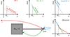 |
Fig. 6. Schematic drawing of complete electron velocity distribution function as measured by EAS instrument on board the Solar Orbiter spacecraft in the case of a positive spacecraft potential decomposed to its individual components: accelerated ambient plasma electrons (red), spacecraft electrons emitted and escaping from far spacecraft surfaces (green), and locally emitted and trapped electrons at the EAS detector (blue). |
In the case of these inter-surface trajectories, electrons are first decelerated moving away from the spacecraft body and accelerated again to their original kinetic energy when moving towards the EAS sensor. Therefore, the sensor does not detect only the local trapped spacecraft electrons below the spacecraft potential and ambient electrons accelerated above the spacecraft potential energy, but also spacecraft electrons with kinetic energies > eΦSC that were originally emitted and escaped from distant spacecraft surfaces – and later became attracted to the EAS detectors. These three different populations (ambient electrons, local trapped spacecraft electrons, and far emitted-escaping and attracted spacecraft electrons) are then contributing to the total measured response of a model EAS sensor, as illustrated in Fig. 6 in red, blue, and green, respectively. Naturally, the trapped and escaping spacecraft electrons at the EAS sensor do not have to follow the same (Maxwellian) distribution shown in our simple schematics; however, the break in the spectrum is, in any case, not necessarily linked to the spacecraft potential value.
Assuming for simplicity that both ambient electrons coming from the solar wind and emitted electrons surrounding the spacecraft are represented by two Maxwellian distributions, as defined in Eqs. (1) and (10) for ne, SW, Te, SW and ne, SC, Te, SC, respectively, their combined spectrum will show a break in the slope at their intersection so that
According to Guillemant (2014), we consider the spacecraft electron population at the location of EAS detectors to be dominated by cold electrons produced by secondary emissions. Using the secondary electron emission yield, ySEE, defined as the ratio of the emitted spacecraft electron flux, Je, SC, and the received ambient electron flux Je, SW, thus giving an average number of emitted particles per one impacting particle as
Here,  refers to the mean thermal velocities of the two populations, we can rewrite Eq. (14) without the density dependency and approximate the Ebreak as a function of electron temperatures only (assuming ySEE is just a function of the surface materials otherwise) as
By considering the spacecraft electron temperature to be independent on the plasma environment – and thus constant in Eq. (16) – we see the energy break, Ebreak, to be an increasing function of the ambient electron temperature, Te, SW.
We tested this possible relation of the Ebreak and the ambient electron temperature by constructing a scatter plot as shown in Fig. 7. We approximated the ambient electron temperature, Te, SW, from the fit of the thermal electrons by use of Eq. (13) for Epeak, SW. In contrast to the spacecraft potential ΦSC (cf., Fig. 5), we now observe an evident correlation where Ebreak value is increasing with Te, SW. From our dataset, we further evaluated the mean spacecraft electron temperature by use of Eq. (13) for Epeak, SC to get

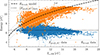 |
Fig. 7. Peak energy for the differential energy flux of spacecraft electrons, Epeak, SC, (blue dots) and energy for the spectrum break between spacecraft and ambient plasma electrons, Ebreak, (orange dots) is plotted as a function of the electron core temperature Te, core. The black dotted line indicates the mean value of Epeak, SC. The black dashed line shows the model dependency of Ebreak for the case of two Maxwellian populations for mean parameters derived from the dataset, the grey dashed lines show the model shifted by the standard deviation, σmodel, of the difference between the model and Ebreak from the dataset. |
similarly, the mean secondary electron emission yield by use of Eq. (16) to get

Inserting the mean values from Eq. (17) and (18) back into Eq. (16), we can evaluate the model energy break Ebreak value as a function of the ambient electron temperature, shown with the black dashed line in Fig. 7. We find a fair agreement between the model and the dataset with a coefficient of determination R2 = 0.54 and a standard deviation of the difference between real and model data of σmodel = σ(Ebreak, data − Ebreak, model)≐0.92 eV. About 80% of all data samples in our dataset fall within a range of ±σmodel, shown in Fig. 7 by a pair of grey dashed lines.
While a continuous increase of Ebreak with ambient electron temperature is predicted by the model given in Eq. (16), we observe in Fig. 7 for higher temperatures a distinct upper limit of Ebreak at about 12 eV. The same limit is well observed for lower spacecraft potential values in Fig. 5. We assume this limit to be possibly an artificial method dependent artefact, rather than a result of any physical process acting at this specific energy level; namely, we suspect the fixed energy limit used to fit the thermal part of the ambient electron population as explained in Sect. 2.2. For higher temperatures – and, thus, rather lower spacecraft potentials – the fixed energy range may be set imprecisely to aptly resolve the thermal part of the ambient electron population at the lowest energies, thus possibly limiting the reliability of the method itself.
The temperature of the spacecraft secondary electrons is typically expected to be about 2 eV (Whipple 1981), while in our case, the estimated temperature from the EAS dataset is observed to be by about 1 eV higher. This discrepancy can be accounted to the EAS performance at very low energies where the measured PSD may have been underestimated, due to very low particle fluxes. This, in turn, can result into an overestimated temperature of the whole spacecraft electron population (so that the peak in differential energy flux is also shifted in energies). Another possible physical explanation is based on the fact that trajectories from the spacecraft body to the EAS detector will preferentially exist for spacecraft electrons with higher energies that are more easily able to escape from the positively charged spacecraft surface and are later attracted back by the EAS detector. This can cause the spacecraft electron population observed by the EAS sensor to be hotter, compared to the population originally emitted by the spacecraft. It is most likely that the estimation of the spacecraft electron temperature will also be affected by the method itself, where the energies below 3 eV end up removed from the analysis; in addition spacecraft electron VDFs are observed to deviate from a simple Maxwellian shape so that also the validity Eq. (13) is limited.
The values of the secondary electron emission yield reported for commonly used spacecraft materials (e.g. Hastings & Garrett 1996) are comparable to those estimated from our dataset. However, we note that the parameter ySEE derived from our dataset is plausibly affected by other effects, for example, by instrument calibration, ambient plasma conditions, or the geometry of the spacecraft structure; in addition, it may become biased by the real value of the secondary electron yield. The secondary electron emission yield is known to depend on the energy of impacting particles. We have compared the derived ySEE parameter to the estimated ambient electron temperature, but no clear correlation is found in our dataset, or for other relevant plasma parameters.
5. Conclusions
In this work, we performed a statistical analysis of a substantial dataset acquired on board the Solar Orbiter mission by the Solar Wind Analyser’s Electron Analyser System. The main focus of this study was to characterise the contamination of the measurements caused by spacecraft-emitted electrons in observed electron velocity distribution functions. We first constructed a model response of an ideal EAS detector to demonstrate the expected properties of spacecraft-emitted electrons at low energies. Based on the model, and as observed on other previously flown space missions, a distinct break, Ebreak, in the energy spectrum of measured phase densities exists at the energy of eΦSC corresponding to the potential ΦSC of the spacecraft. Below Ebreak, the measurements are acquired due to cold spacecraft emitted electrons only while the full ambient electron population is observed shifted in energies above eΦSC.
As demonstrated on a real VDF data sample, a similar energy break in the spectrum also exists in the case of SWA-EAS measurements on board Solar Orbiter. However, the transition between the spacecraft and ambient electrons is found to be rather smooth – and not as a distinct cut-off separating the two parts of the measured spectrum. To statistically assess the properties of the break in measured spectra, we developed an automated method to localise the position of Ebreak. By employing this method on a large dataset we analysed possible correlations of derived Ebreak to the spacecraft potential. We concluded that in the case of SWA-EAS measurements, no distinct correlation of Ebreak with ΦSC is found in our results, and, moreover, the measured electron VDFs are indicated to be contaminated by the cold spacecraft electron emissions even at energies well above eΦSC. This finding is contrary to what is seen in the model EAS response and to observations from other previous missions as well.
We propose a plausible explanation for this discrepancy based on the geometry of the spacecraft structure. We argue that spacecraft electrons with energies above eΦSC can be observed by SWA-EAS as a result of emission sources with their locations far away from the instruments itself. Such particle trajectories have been plausibly shown to exist in prior numerical simulation studies. Assuming the detection of far emitted spacecraft electron populations, we derived a theoretical form of Ebreak as a function of the temperature of the ambient thermal electron population. We found a good agreement between the real SWA-EAS measurements and this hypothesis. For the SWA-EAS electron measurements, the spacecraft potential value measured by RPW is therefore inappropriate as a limit for excluding the spacecraft electrons from subsequent data analysis. Instead, to apply any empirical safety margins, the Ebreak dependency on the ambient electron temperature may provide a reliable threshold for removing spacecraft electrons effects when processing the SWA-EAS measurements to any higher level scientific data products.
Although the proposed explanation for the observation of spacecraft electrons above the spacecraft potential threshold is found to be compliant with the derived properties of Ebreak, the SWA-EAS observations do not provide a direct proof for this scenario. This is because it is impossible to distinguish individual electron fluxes from different sources in real measured data. As an additional verification, we plan to extend the current study by using numerical simulations following previous works carried out within the Spacecraft Interaction System (SPIS) framework (Guillemant et al. 2012; Guillemant 2014; Guillemant et al. 2017). In this approach, the different electron populations can be treated separately, even down to individual particle trajectories, enabling the decomposition of the total VDFs (as measured by virtual detectors) to localised sources. In addition, this approach may also aid in the identification of some specific patterns in the energy spectra, when compared to real measured data samples from SWA-EAS experiments.
ESA Solar Orbiter Archive is available at http://soar.esac.esa.int.
Acknowledgments
Solar Orbiter is a space mission of international collaboration between ESA and NASA, operated by ESA. Solar Orbiter Solar Wind Analyser (SWA) data are derived from scientific sensors which have been designed and created, and are operated under funding provided in numerous contracts from the UK Space Agency (UKSA), the UK Science and Technology Facilities Council (STFC), the Agenzia Spaziale Italiana (ASI), the Centre National d’Etudes Spatiales (CNES, France), the Centre National de la Recherche Scientifique (CNRS, France), the Czech contribution to the ESA PRODEX programme, and NASA. Solar Orbiter SWA work at UCL/MSSL is currently funded under STFC grants ST/W001004/1 and ST/X/002152/1. This work was supported by the Czech Science Foundation (GAČR), project No. 23-07334S. The authors further acknowledge intense collaboration with the SWA-EAS and RPW instrument teams when discussing any technical, calibration, or data product related issues.
References
- Barrie, A. C., Cipriani, F., Escoubet, C. P., et al. 2019, Phys. Plasmas, 26, 103504 [NASA ADS] [CrossRef] [Google Scholar]
- Berry Garrett, H. 1981, Rev. Geophys. Space Phys., 19, 577 [CrossRef] [Google Scholar]
- Bouhram, M., Dubouloz, N., Hamelin, M., et al. 2002, Ann. Geophys., 20, 365 [NASA ADS] [CrossRef] [Google Scholar]
- Feldman, W. C., Asbridge, J. R., Bame, S. J., Montgomery, M. D., & Gary, S. P. 1975, J. Geophys. Res., 80, 4181 [Google Scholar]
- Feldman, W. C., Asbridge, J. R., Bame, S. J., & Gosling, J. T. 1979, J. Geophys. Res., 84, 7371 [NASA ADS] [CrossRef] [Google Scholar]
- Geach, J., Schwartz, S. J., Génot, V., et al. 2005, Ann. Geophys., 23, 931 [NASA ADS] [CrossRef] [Google Scholar]
- Génot, V., & Schwartz, S. J. 2004, Ann. Geophys., 22, 2073 [CrossRef] [Google Scholar]
- Grard, R. J. L. 1973, J. Geophys. Res., 78, 2885 [NASA ADS] [CrossRef] [Google Scholar]
- Guillemant, S. 2014, Theses, Université Paul Sabatier– Toulouse III, France [Google Scholar]
- Guillemant, S., Génot, V., Matéo-Vélez, J.-C., Ergun, R., & Louarn, P. 2012, Ann. Geophys., 30, 1075 [NASA ADS] [CrossRef] [Google Scholar]
- Guillemant, S., Maksimovic, M., Hilgers, A., et al. 2017, IEEE Trans. Plasma Sci., 45, 2578 [CrossRef] [Google Scholar]
- Hamelin, M., Bouhram, M., Dubouloz, N., et al. 2002, Ann. Geophys., 20, 377 [NASA ADS] [CrossRef] [Google Scholar]
- Hastings, D., & Garrett, H. 1996, Spacecraft-Environment Interactions, Cambridge Atmospheric and Space Science Series (Cambridge University Press) [Google Scholar]
- Hutchinson, I. H. 2002, Principles of Plasma Diagnostics, 2nd edn. (Cambridge University Press) [CrossRef] [Google Scholar]
- Issautier, K., Meyer-Vernet, N., Moncuquet, M., & Hoang, S. 1998, J. Geophys. Res., 103, 1969 [NASA ADS] [CrossRef] [Google Scholar]
- Khotyaintsev, Y. V., Graham, D. B., Vaivads, A., et al. 2021, A&A, 656, A19 [NASA ADS] [CrossRef] [EDP Sciences] [Google Scholar]
- Langmuir, I., & Blodgett, K. B. 1924, Phys. Rev., 24, 49 [NASA ADS] [CrossRef] [Google Scholar]
- Lavraud, B., & Larson, D. E. 2016, J. Geophys. Res., 121, 8462 [NASA ADS] [CrossRef] [Google Scholar]
- Lewis, G. R., André, N., Arridge, C. S., et al. 2008, Planet. Space Sci., 56, 901 [NASA ADS] [CrossRef] [Google Scholar]
- Lindqvist, P. A., Olsson, G., Torbert, R. B., et al. 2016, Space Sci. Rev., 199, 137 [NASA ADS] [CrossRef] [Google Scholar]
- Maksimovic, M., Gary, S. P., & Skoug, R. M. 2000, J. Geophys. Res., 105, 18337 [NASA ADS] [CrossRef] [Google Scholar]
- Maksimovic, M., Zouganelis, I., Chaufray, J. Y., et al. 2005, J. Geophys. Res., 110, A09104 [NASA ADS] [Google Scholar]
- Maksimovic, M., Bale, S. D., Chust, T., et al. 2020, A&A, 642, A12 [EDP Sciences] [Google Scholar]
- Maksimovic, M., Souček, J., Chust, T., et al. 2021, A&A, 656, A41 [NASA ADS] [CrossRef] [EDP Sciences] [Google Scholar]
- Marsch, E. 2006, Liv. Rev. Sol. Phys., 3, 1 [Google Scholar]
- Montgomery, M. D., Bame, S. J., & Hundhausen, A. J. 1968, J. Geophys. Res., 73, 4999 [NASA ADS] [CrossRef] [Google Scholar]
- Mott-Smith, H. M., & Langmuir, I. 1926, Phys. Rev., 28, 727 [CrossRef] [Google Scholar]
- Müller, D., St. Cyr, O. C., & Zouganelis, I. 2020, A&A, 642, A1 [NASA ADS] [CrossRef] [EDP Sciences] [Google Scholar]
- Nicolaou, G., & Livadiotis, G. 2016, Ap&SS, 361, 359 [NASA ADS] [CrossRef] [Google Scholar]
- Nicolaou, G., Wicks, R., Livadiotis, G., et al. 2020, Entropy, 22, 212 [NASA ADS] [CrossRef] [Google Scholar]
- Nicolaou, G., Wicks, R. T., Owen, C. J., et al. 2021, A&A, 656, A10 [NASA ADS] [CrossRef] [EDP Sciences] [Google Scholar]
- Ogilvie, K. W., & Scudder, J. D. 1978, J. Geophys. Res., 83, 3776 [Google Scholar]
- Owen, C. J., Bruno, R., Livi, S., et al. 2020, A&A, 642, A16 [EDP Sciences] [Google Scholar]
- Pedersen, A. 1995, Ann. Geophys., 13, 118 [NASA ADS] [CrossRef] [Google Scholar]
- Pedersen, A., Lybekk, B., André, M., et al. 2008, J. Geophys. Res., 113 [Google Scholar]
- Phillips, J., Bame, S., Gosling, J., et al. 1993, Adv. Space Res., 13, 47 [NASA ADS] [CrossRef] [Google Scholar]
- Pilipp, W. G., Miggenrieder, H., Montgomery, M. D., et al. 1987, J. Geophys. Res., 92, 1075 [Google Scholar]
- Pilipp, W. G., Muehlhaeuser, K.-H., Miggenrieder, H., Rosenbauer, H., & Schwenn, R. 1990, J. Geophys. Res., 95, 6305 [NASA ADS] [CrossRef] [Google Scholar]
- Pulupa, M. P., Bale, S. D., Salem, C., & Horaites, K. 2014, J. Geophys. Res., 119, 647 [NASA ADS] [CrossRef] [Google Scholar]
- Rosenbauer, H., Schwenn, R., Marsch, E., et al. 1977, J. Geophys. Zeitschr. Geophys., 42, 561 [NASA ADS] [Google Scholar]
- Salem, C., Bosqued, J.-M., Larson, D. E., et al. 2001, J. Geophys. Res., 106, 21701 [NASA ADS] [CrossRef] [Google Scholar]
- Salem, C. S., Pulupa, M., Bale, S. D., & Verscharen, D. 2023, A&A, 675, A162 [NASA ADS] [CrossRef] [EDP Sciences] [Google Scholar]
- Scime, E. E., Bame, S. J., Feldman, W. C., et al. 1994a, J. Geophys. Res., 99, 23401 [Google Scholar]
- Scime, E. E., Phillips, J. L., & Bame, S. J. 1994b, J. Geophys. Res., 99, 14769 [NASA ADS] [CrossRef] [Google Scholar]
- Scudder, J. D., Cao, X., & Mozer, F. S. 2000, J. Geophys. Res., 105, 21281 [NASA ADS] [CrossRef] [Google Scholar]
- Song, P., Zhang, X., & Paschmann, G. 1997, Planet. Space Sci., 45, 255 [CrossRef] [Google Scholar]
- Steinvall, K., Khotyaintsev, Y. V., Cozzani, G., et al. 2021, A&A, 656, A9 [NASA ADS] [CrossRef] [EDP Sciences] [Google Scholar]
- Štverák, Š., Maksimovic, M., Trávníček, P. M., et al. 2009, J. Geophys. Res., 114, A05104 [Google Scholar]
- Štverák, Š., Trávníček, P. M., & Hellinger, P. 2015, J. Geophys. Res., 120, 8177 [Google Scholar]
- Verscharen, D., Klein, K. G., & Maruca, B. A. 2019, Liv. Rev. Sol. Phys., 16, 5 [Google Scholar]
- Verscharen, D., Chandran, B. D. G., Boella, E., et al. 2022, Front. Astron. Space Sci., 9, 951628 [NASA ADS] [CrossRef] [Google Scholar]
- Whipple, E. C. 1981, Rep. Prog. Phys., 44, 1197 [NASA ADS] [CrossRef] [Google Scholar]
- Wilson, L. B., Salem, C. S., & Bonnell, J. W. 2023, ApJS, 269, 52 [NASA ADS] [CrossRef] [Google Scholar]
- Zouganelis, I., De Groof, A., Walsh, A. P., et al. 2020, A&A, 642, A3 [NASA ADS] [CrossRef] [EDP Sciences] [Google Scholar]
All Figures
|
Fig. 1. Radial coverage (black line) and SWA-EAS data availability (green dots) shown as a function of time along the Solar Orbiter trajectory in the year 2021. |
| In the text | |
|
Fig. 2. Statistical properties of the dataset used in the present study. Histograms show (a) number of time-averaged data samples for the radial distance from the Sun; (b) spacecraft potential as derived from RPW measurements; (c) solar wind proton densities; and (d) solar wind proton bulk speeds received from PAS on ground moments. |
| In the text | |
|
Fig. 3. Comparison between the model and measured data for an ideal Electron Analyser System (EAS) sensor. (a) The model phase space density as a function of energy. The contribution of the ambient solar wind electrons in the plasma reference frame (PRF) is shown as the black solid line. The red dots display the ambient electron distribution as seen by the individual FOV bins of an ideal EAS detector in the spacecraft reference frame (SRF). The contribution of the spacecraft emitted electrons trapped by the spacecraft potential (escaping away from the detector) is shown by the blue (green) dots. Black empty circles display the modelled EAS response averaged for each energy over all FOV directions of the instrument. The yellow line display the contribution of the ambient electron distribution modified by the spacecraft potential energy (denoted by the black dotted line). Panel b translates the results of panel a into differential energy fluxes. (c) Real EAS data samples in phase space densities (grey dots) in a format similar to panel a. The fitted contributions of the ambient, spacecraft, and all electrons as a function of energy. plotted with red, blue, and black dashed lines, respectively. Panel d recast the results of panel c in differential energy fluxes. For further reference we show in panel d the big blue, orange, and red circles the estimated peak differential energy flux of the spacecraft electrons Epeak, SC (big blue circle), the position of the break Ebreak (big orange circle), and the estimated peak of the differential energy flux of the solar wind electrons Epeak, SW (big red circle). |
| In the text | |
|
Fig. 4. Scatter plot of RPW spacecraft potential as a function of proton density derived from PAS measurements (green dots). Data are over-plotted by a theoretical profile (dashed line) computed using Eq. (A7) in Salem et al. (2001). |
| In the text | |
|
Fig. 5. Peak energy for the differential energy flux of spacecraft electrons Epeak, SC (blue dots) and energy for the spectrum break between spacecraft and ambient plasma electrons Ebreak (orange dots) is plotted as a function of the RPW spacecraft potential ΦSC. The black line shows the axis E = eΦSC corresponding to the expected correlation between Ebreak and ΦSC. |
| In the text | |
|
Fig. 6. Schematic drawing of complete electron velocity distribution function as measured by EAS instrument on board the Solar Orbiter spacecraft in the case of a positive spacecraft potential decomposed to its individual components: accelerated ambient plasma electrons (red), spacecraft electrons emitted and escaping from far spacecraft surfaces (green), and locally emitted and trapped electrons at the EAS detector (blue). |
| In the text | |
|
Fig. 7. Peak energy for the differential energy flux of spacecraft electrons, Epeak, SC, (blue dots) and energy for the spectrum break between spacecraft and ambient plasma electrons, Ebreak, (orange dots) is plotted as a function of the electron core temperature Te, core. The black dotted line indicates the mean value of Epeak, SC. The black dashed line shows the model dependency of Ebreak for the case of two Maxwellian populations for mean parameters derived from the dataset, the grey dashed lines show the model shifted by the standard deviation, σmodel, of the difference between the model and Ebreak from the dataset. |
| In the text | |
Current usage metrics show cumulative count of Article Views (full-text article views including HTML views, PDF and ePub downloads, according to the available data) and Abstracts Views on Vision4Press platform.
Data correspond to usage on the plateform after 2015. The current usage metrics is available 48-96 hours after online publication and is updated daily on week days.
Initial download of the metrics may take a while.