| Issue |
A&A
Volume 693, January 2025
|
|
|---|---|---|
| Article Number | A131 | |
| Number of page(s) | 10 | |
| Section | Catalogs and data | |
| DOI | https://doi.org/10.1051/0004-6361/202451987 | |
| Published online | 10 January 2025 | |
Photometric analysis of 40 low mass-ratio contact binary systems in the Catalina Sky Survey
1
Yunnan Observatories, Chinese Academy of Sciences,
Kunming
650216,
PR China
2
University of Chinese Academy of Sciences,
Beijing
100049,
PR China
3
Key Laboratory of the Structure and Evolution of Celestial Objects, Chinese Academy of Sciences,
PO Box 110,
650216
Kunming,
PR China
4
Center for Astronomical Mega-Science, Chinese Academy of Sciences,
20A Datun Road, Chaoyang District,
Beijing
100012,
PR China
5
College of Physics and Electronic Engineering, Xingtai University,
Xingtai
054001,
PR China
★ Corresponding author; This email address is being protected from spambots. You need JavaScript enabled to view it.
Received:
26
August
2024
Accepted:
20
November
2024
Abstract
Low mass-ratio contact binary systems are a fascinating class of eclipsing binaries; they are widely regarded as the potential progenitors of stellar mergers. For this study we analyzed 40 newly discovered low mass-ratio totally eclipsing contact binary systems identified from the Catalina Sky Survey data. The relative parameters for these systems were inferred using a neural network model combined with a Bayesian inference-based Hamiltonian Monte Carlo (HMC) algorithm, with uncertainties estimated from the posterior distributions generated by the HMC algorithm. The absolute parameters were then calculated using these relative parameters, along with distances and temperatures provided by Gaia Data Release 3. Among the 40 systems, 24 are deep low mass-ratio overcontact binaries, characterized by fill-out factors of 0.5 or higher and mass ratios of 0.25 or lower. Notably, two systems, CSS_J071952.5+243224 and CSS_J155519.0+135855, have mass ratios below 0.1, specifically 0.094 ± 0.006 and 0.086 ± 0.004, respectively. Furthermore, we compared the parameters obtained in this study with those from 39 low mass-ratio contact binary systems identified in previous research, finding that the estimated parameters are largely consistent. Finally, to evaluate the evolutionary status of the 40 systems, we calculated the ratio of spin angular momentum to orbital angular momentum for each and found that all are currently in a relatively stable evolutionary phase.
Key words: methods: data analysis / techniques: photometric / binaries: close / stars: evolution
© The Authors 2025
 Open Access article, published by EDP Sciences, under the terms of the Creative Commons Attribution License (https://creativecommons.org/licenses/by/4.0), which permits unrestricted use, distribution, and reproduction in any medium, provided the original work is properly cited.
This article is published in open access under the Subscribe to Open model. This email address is being protected from spambots. You need JavaScript enabled to view it. to support open access publication.
1 Introduction
Contact binary systems, also referred to as EW-type or W Ursae Majoris (W UMa) systems, are crucial astrophysical objects for studying stellar evolution and interaction. The leading theory suggests that these systems originate from initially detached binaries that gradually lose angular momentum through magnetic wind, ultimately leading to their contact configuration (Vilhu 1982; Maceroni & van’t Veer 1996; McCarthy et al. 1996; Qian 2003). Typically composed of two late-type stars, these systems exhibit intense mass and energy exchange, with both components filling their Roche lobes and sharing a common envelope (Kopal 1959; Lucy & Wilson 1979). The close separation between the components leads to relatively brief orbital periods; the majority of these systems display periods concentrated within the range of 0.25 to 0.5 days. This proximity is manifested in the variability in their light curves, which serves as a potent means of investigating the formation and evolutionary processes of contact binary systems (Sun et al. 2020).
Low mass-ratio contact binary systems and their potential mergers may give rise to peculiar stellar types, such as FK Com stars and blue stragglers (Rasio 1995; Qian et al. 2006). When the mass ratio drops below a certain theoretical threshold (qmin), a Darwin instability (Huang 1966; Hut 1980) is triggered, leading the contact binary system to merge into a single star. Yang & Qian (2015) estimated that q could be as low as 0.044. Recent statistical findings by Pešta & Pejcha (2023) suggest that for late-type contact binary systems with periods exceeding 0.3 days, q is approximately 0.087. V1309 Sco is an observational example of a low mass-ratio contact binary merger and is classified as a red nova (Tylenda et al. 2011). The progenitor of V1309 Sco was an eclipsing contact binary with an extremely low mass-ratio and an orbital period of 1.4 days, consisting of an early-type subgiant and a low-mass companion (Stȩpień 2011; Nandez et al. 2014). Kochanek et al. (2014) estimated that events similar to the stellar merger of V1309 Sco occur in the Galaxy at a frequency of roughly once per decade. Therefore, identifying candidate systems with low or extremely low mass-ratios before they merge is crucial for advancing our understanding of the mechanisms driving contact binary mergers. Research focusing on these systems not only enhances our ability to monitor impending merger events, but also deepens our insight into the limits and processes involved in such stellar phenomena.
In recent years, advancements in large-scale time-domain surveys have greatly expanded the catalog of contact binary systems with low mass-ratios. For example, Christopoulou et al. (2022) investigated 30 candidates of low mass-ratio contact binary systems from the Catalina Sky Survey (CSS; Drake et al. 2009), Li et al. (2022) analyzed 10 candidates from the All Sky Automated Survey (ASAS; Pojmanski 1997), Liu et al. (2023) investigated 11 candidates from the catalog provided by Sun et al. (2020), Cheng et al. (2024) conducted a detailed analysis of 2 candidates from the Transiting Exoplanet Survey Satellite (TESS; Ricker et al. 2015), and Lalounta et al. (2024) provided 9 candidates from the CSS.
This study focuses on the catalog of relative parameters for 5172 contact binary systems provided by Wang et al. (2024) from the CSS, identifying 40 new low mass-ratio contact binary systems with total eclipses and conducting a detailed analysis of them. In Section 2 we describe the data sources and provide an overview of the basic information. Section 3 outlines the methodology used to derive the light curve parameters. In Section 4 we determine both the relative and absolute parameters of the systems and discuss them. Finally, in Sect. 5 we present a summary and our conclusions.
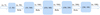 |
Fig. 1 Neural network architecture used in this study. The input layer is (n, 5), with n as 150 000 training samples and 5 input parameters: T1, i, q., f, and T2/T1. The output layer is (n, 100), representing the synthetic light curve with 100 phase points. The hidden layers contain 50, 500, and 200 nodes, respectively. The Relu activation function (Nair & Hinton 2010) introduces nonlinearity to the model. |
2 Data
Wang et al. (2024) conducted a photometric analysis of 5172 late-type contact binaries sourced from the CSS and derived their parameters. Of these, 726 systems were found to have mass ratios below 0.2. By visually inspecting the light curves of these 726 systems, we selected 40 totally eclipsing contact binary systems with high signal-to-noise ratios. The basic information for these 40 systems is presented in Table A.1. The basic information included in Table A.1 comprises the CSS ID, the coordinates (including RA (J2000) and Dec (J2000)), the period (day), and the V-band maximum magnitude (mag) of these systems. All of this information was sourced from Drake et al. (2014). To ensure consistency in the dimensions of the observed light curves with those generated by the PHysics Of Eclipsing BinariEs (PHOEBE; Prša & Zwitter 2005; Prša et al. 2016; Conroy et al. 2020) software, and to facilitate faster convergence of the neural network model, we subtracted the mean value from each observed light curve. That is,  .
.
3 Light curve solutions
We employed the method proposed by Wang et al. (2024) to derive the relative parameters and their uncertainties for 40 low mass-ratio contact binary systems. These parameters include orbital inclination (i), mass ratio (q), fill-out factor (f), and effective temperature ratio (T2/T1). The approach integrates a neural network model with the Hamiltonian Monte Carlo (HMC; Hoffman et al. 2014) algorithm from Bayesian inference, enabling rapid and efficient determination of these parameters and their uncertainties for large numbers of contact binary systems. The neural network model serves as a substitute for the PHOEBE software, facilitating the quick generation of synthetic light curves and expediting the subsequent inference process using the HMC algorithm. The HMC algorithm was then utilized to infer the relative parameters from the light curves in bulk, providing posterior distributions for these parameters, from which the uncertainties are statistically determined.
To build and train a neural network model that maps parameters to synthetic light curves, a large dataset matching parameters with corresponding synthetic light curves is required. These samples were generated using the PHOEBE software, resulting in a total of 170000 sets of parameters and their corresponding synthetic light curves. Out of these, 150000 were used for training the neural network model, 10 000 for validation, and the remaining 10000 for testing. The framework of the neural network model is illustrated in Fig. 1. In this figure, the input layer is described as (n, 5), where n denotes the number of training samples, which in this case is 150 000, and 5 represents the number of input parameters, namely T1, i, q, f, and T2/T1. The output layer is denoted as (n, 100), where 100 indicates the synthetic light curve with 100 phase points. The hidden layers are positioned between the input and output layers, with 50, 500, and 200 indicating the number of nodes in each hidden layer, the rectified linear unit (Relu; Nair & Hinton 2010) is the activation function providing nonlinearity to the model. The trained neural network model was used to predict the synthetic light curves for the 10 000 samples in the test set, and the standard deviation of the residuals between each predicted light curve and the actual light curve was calculated. It was found that the standard deviation of the residuals is primarily distributed  , which is significantly lower than the photometric errors of the CSS (Drake et al. 2013), thus meeting the required accuracy. A comparison between two light curves generated by the neural network model and the PHOEBE software is shown in Figure 2. In the upper portion of the figure the blue line represents the light curve produced by the PHOEBE software, while the orange line corresponds to the light curve generated by the neural network model. The lower portion of the figure displays the residuals between the two curves in blue, with the red dashed line indicating the zero-value reference. For the light curve in the upper left, the corresponding parameters were T1 = 5382 K, i = 78°.35, q = 0.084, f = 0.36, and T2/T1 = 0.852. For the light curve in the upper right, the associated parameters were T1 = 7516 K, i = 85º.76, q = 0.130, f = 0.63, and T2/T1 = 0.940. As shown in Figure 2, the light curves predicted by the neural network model closely align with those generated by the PHOEBE software. The residuals are tightly clustered around the zero baseline, demonstrating that using the neural network model as a substitute for the PHOEBE software in generating light curves is entirely feasible. On a computer equipped with 16 GB of random-access memory (RAM) and a 16-core CPU operating at 3.4 GHz, the trained neural network model generates synthetic light curves with 100 phase points in an average of 0.001 seconds. In contrast, under identical conditions, the PHOEBE software requires an average of 5 seconds for the same task. This performance disparity indicates that the neural network model processes light curves approximately four orders of magnitude faster than the PHOEBE software, thereby significantly accelerating the subsequent parameter inference process.
The HMC algorithm is a powerful and efficient Markov chain Monte Carlo (MCMC) method that can infer the parameters of a large number of light curves in bulk. This makes it highly suitable for deriving the parameters of massive light curve datasets released by large-scale time-domain surveys.
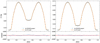 |
Fig. 2 Comparison between the synthetic light curves generated by the neural network model and those produced by PHOEBE is presented. The upper panel shows the light curve generated by PHOEBE (blue line) and the one produced by the neural network model (orange line). The lower panel presents the residuals between the two curves (blue), with the red dashed line indicating the zero reference. |
4 Result and discussion
4.1 Relative parameters
It is assumed that the influence of the third-light component can be disregarded. The presence of any third component has no effect on the estimation of relative parameters (including the inclination and mass ratio), it only affects luminosity and mass. D’Angelo et al. (2006) studied the third component in their contact binary system sample, and the results showed that the uncertainty of the third component to its total luminosity was less than 0.15 mag, and the uncertainty of the derived mass was only increased by about 3%. We used the neural network model combined with the HMC algorithm (Wang et al. 2024) to derive the relative parameters for 40 low mass-ratio contact binary systems. The estimated relative parameters and their uncertainties for these systems are listed in Table A.2, where the mass ratios are all below 0.2. To further validate the parameter estimates, we input the estimated values for each system into the PHOEBE software to generate the corresponding light curves. The quality of these estimates was evaluated by calculating the goodness of fit (R2) between the newly generated light curves and the observed ones. The values of R2 range from 0 to 1; values closer to 1 indicate more accurate parameter estimates. The formula for calculating R2 is as follows:
 (1)
(1)
Here m represents the number of data points in the light curve, yj denotes the observed value at the j-th data point, ŷj represents the predicted value at the j-th data point, and ӯ denotes the mean of all observed values in the light curve.
The R2 values for all 40 systems range from 0.89 to 0.97, indicating a strong fit across the board. To provide a more visual demonstration of the fitting quality for low mass-ratio contact binary systems with varying R2 values, we randomly selected eight targets from the 40 systems for illustration.
Figure 3 shows two targets (CSS_J042157.5−001751 and CSS_J024234.7+054412) with R2 values between 0.95 and 0.97; Figure A.1 displays two targets (CSS_J013700.4−081228 and CSS_J044336.7+041144) with R2 values between 0.93 and 0.95; Figure A.2 presents two targets (CSS_J025611.5+324252 and CSS_J143416.4−173841) with R2 values between 0.91 and 0.93; and Figure A.3 illustrates two targets (CSS_J162227.3−063725 and CSS_J095456.8−123840) with R2 values between 0.89 and 0.91. In Figures 3, A.1, A.2, and A.3, the observed light curves are represented by blue dots and gray lines, which include photometric errors, while the orange lines correspond to the light curves generated by inputting the estimated parameters into the PHOEBE software. The subplot titles indicate the IDs of the systems and their respective R2 values. The figures demonstrate that the higher-quality observed light curves are associated with larger R2 values. Figure 4 shows the posterior distributions of the parameters for the first target (CSS_J042157.5−001751) in Figure 3, while Figure A.4 displays the posterior distributions of the parameters for the first target (CSS_J162227.3−063725) in Figure A.3. In Figures 4, and A.4, in each of the four diagonal panels, the solid vertical lines represent the median (50th percentile) of the parameter distribution. The two dashed vertical lines flanking the median indicate the lower and upper bounds of the 68% credible interval, which corresponds to the innermost contour in the six off-diagonal panels. The statistical values for this interval are presented in the first row above the four diagonal panels. The outermost dotted vertical lines in the diagonal panels mark the lower and upper bounds of the 95% credible interval, corresponding to the outer contour in the six off-diagonal panels, with the associated statistical values shown in the second row above the diagonal panels. These posterior distributions allow us to determine the uncertainties of the parameters.
Based on the statistical results of Pešta & Pejcha (2023), the minimum mass ratio (qmin) for late-type contact binary systems with orbital periods greater than 0.3 days is  . In our sample, 36 of the 40 newly identified low mass-ratio systems have periods exceeding 0.3 days, with the lowest observed q value being 0.086, which lies within the 3σ range (0.042−0.159) reported by Pešta & Pejcha (2023). For late-type binaries with shorter periods, Pešta & Pejcha (2023) report a minimum mass ratio of
  . Among our newly discovered systems, four have periods less than or equal to 0.3 days, with the lowest observed q value being 0.149, also within the 3σ range (0.108−0.333) established by Pešta & Pejcha (2023). These findings are in agreement with the statistical results of Pešta & Pejcha (2023), supporting the reliability of the mass ratios determined in our sample.
Christopoulou et al. (2022) and Lalounta et al. (2024) determined the parameters for 30 and 9 low mass-ratio contact binary systems from the CSS, respectively. We applied the method of Wang et al. (2024) to determine the parameters for these 39 systems and compared them with those obtained by Christopoulou et al. (2022) and Lalounta et al. (2024). The comparison of the four parameters is shown in Figure 5, where the blue dots represent the comparison with the parameters provided by Christopoulou et al. (2022) for 30 systems, and the red dots represent the comparison with the parameters provided by Lalounta et al. (2024) for 9 systems. The orange dashed line indicates the 45 degree line. As depicted in the figure, the parameter values are largely distributed near the 45 degree line, further validating the reliability of our results.
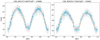 |
Fig. 3 Fitting results for CSS_J042157.5−001751 and CSS_J024234.7+054412 are shown. The blue dots and gray lines represent the observed light curves with photometric errors, while the orange lines depict the light curves generated using the estimated parameters input into the PHOEBE software. |
 |
Fig. 4 Posterior distribution of the four parameters (i, q, f, and T2/T1) for CSS_J042157.5−001751 derived using the proposed method. In each diagonal panel the solid vertical line represents the median (50th percentile) of the parameter distribution. The dashed lines indicate the 68% credible interval, while the dotted lines mark the 95% credible interval. These intervals are also reflected in the off-diagonal contour plots, with the corresponding statistical values provided above the diagonal panels, helping to determine parameter uncertainties. |
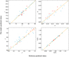 |
Fig. 5 Comparison of the four parameters (i, q, f, and T2/T1). The blue dots correspond to 30 systems from Christopoulou et al. (2022), and the red dots to 9 systems from Lalounta et al. (2024). The orange dashed line represents the 45 degree line. |
4.2 Absolute parameters
Based on the method proposed by Poro et al. (2022, 2024), combined with the relative parameters derived from the light curves, we present the absolute parameters for 40 low mass-ratio contact binary systems that were determined:
Step 1: Calculation of the absolute magnitudes (Mv) of these systems using the following formula:
 (2)
(2)
Here, V represents the magnitude in the V-band, d is the distance obtained from Gaia DR3 (Gaia Collaboration 2023), and AV is the extinction coeffificient calculated using the DUST-MAPS PYTHON package (Green et al. 2019).
Step 2: Calculation of the absolute magnitudes (Mv(1,2)) of the primary and secondary stars using the following formula:
 (3)
(3)
Here L1 and L2 represent the luminosities of the primary and secondary stars, respectively, and L(1,2)/(L1 + L2) can be calculated from the relative luminosity ratio (L2/L1).
Step 3: Calculation of the bolometric magnitudes (Mbol(1,2)) of the primary and secondary stars using the following formula:
 (4)
(4)
Here BC(1,2) is the bolometric correction, obtained from Pecaut & Mamajek (2013).
Step 4: Calculation of the luminosities (L(1,2)) of the primary and secondary stars using the following formula:
 (5)
(5)
Here  is the solar bolometric magnitude, taken as 4.73 mag (Torres 2010).
Step 5: Estimation of the mass (M1) of the primary based on its luminosity (Christopoulou et al. 2022; Papageorgiou et al. 2023). The mass (M2) of the secondary is subsequently determined using the mass ratio (q = M2/M1). The calculation formulas are as follows:
 (6)
(6)
Step 6: Calculation of the semimajor axis (a) of the system using Kepler’s third law (Panchal & Joshi 2021) with the following formula:
 (7)
(7)
Here G is the gravitational constant, and P is the period of the system.
Step 7: Calculation of the radii (R(1,2)) of the primary and secondary stars using the relative radii (r(1,2)) with the following formula:
 (8)
(8)
By integrating these seven steps, we determined the absolute parameters for the 40 systems, as shown in Table A.3, with the primary temperatures coming from Gaia DR3 (Gaia Collaboration 2023).
 |
Fig. 6 Variation in Js/Jo with q for 40 systems. The orange points illustrate the Js/Jo values for the 40 low mass-ratio contact binary systems identified in this study, while the blue points represent the 30 systems reported by Christopoulou et al. (2022), and the red points correspond to the 9 systems discovered by Lalounta et al. (2024). The gray dashed line marks the instability threshold at Js/Jo = 1/3. |
4.3 The stability analysis
In Section 1, we show that extremely low mass-ratio contact binary systems are likely progenitors of merging stars, such as blue stragglers and FK Com stars. As Hut (1980) explained, a binary system becomes susceptible to tidal (Darwin) instability when the ratio of the total spin angular momentum (Js) to the orbital angular momentum (Jo) exceeds approximately 1/3. Under this condition, the system becomes unstable, and leads to a merger as the secondary star can no longer maintain the synchronous rotation of the primary star through tidal interactions. Here we investigate the evolutionary status of the 40 target systems to assess their susceptibility to this instability. We calculate Js/Jo using the formula provided by Li & Zhang (2006) as follows:
![Mathematical equation: ${{{J_{\rm{s}}}} \over {{J_{\rm{o}}}}} = {{(1 + q)} \over q}{\left( {{k_1}{r_1}} \right)^2}\left[ {1 + q{{\left( {{{{k_2}} \over {{k_1}}}} \right)}^2}{{\left( {{{{r_2}} \over {{r_1}}}} \right)}^2}} \right].$](/articles/aa/full_html/2025/01/aa51987-24/aa51987-24-eq14.png) (9)
(9)
The mass ratio is denoted by q, with r1 and r2 representing the relative radii, and k1 and k2 the dimensionless gyration radii. Since the values of k1 and k2 are influenced by the star’s internal structure, an accurate determination of these radii is essential for the precise calculation of the Js/Jo value. We initially assumed  (Sun-like; Rasio 1995; Li & Zhang 2006), and the calculated Js/Jo values for the 40 systems are shown in the left panel of Figure 6. The orange points represent the Js/Jo values for the 40 low mass-ratio contact binary systems newly identified in this study, the blue points correspond to the 30 systems discovered by Christopoulou et al. (2022), and the red points denote the 9 systems found by Lalounta et al. (2024). The gray dashed line indicates the instability threshold at Js/Jo = 1/3. As seen in the figure, all 40 systems have Js/Jo values below 1/3, indicating that they are in a stable state. To further refine the values of k1 and k2, we recalculated k1 for primary components of varying masses, utilizing the tabulated data from Landin et al. (2009), which account for the influences of tidal and rotational distortions on stars within binary systems. We determined k1 using the following linear equations: for stars with masses between 0.5 and 1.4 M⊙, k1 = −0.250 M + 0.539, and for stars with masses greater than 1.4 M⊙, k1 = 0.014 M + 0.152. For the secondary component, we adopted
  , consistent with the value for a fully convective star (Arbutina 2007). This assumption is justified given that the secondary is a very low-mass star (M2 < 0.3 M⊙). The calculated values of Js/Jo for the 40 systems are displayed in the right panel of Figure 6.
5 Summary and conclusions
In this paper we investigated 40 newly identified totally eclipsing low mass-ratio contact binary systems from the CSS (Drake et al. 2014), selected from the catalog provided by Wang et al. (2024). To infer the relative parameters and their uncertainties, such as the mass ratio q, orbital inclination i, fill-out factor f, and temperature ratio T2/T1, we employed a neural network model combined with the HMC algorithm (Hoffman et al. 2014), based on Bayesian inference. Subsequently, we determined the absolute parameters of these systems, including the luminosities L(1,2), masses M(1,2), and radii R(1,2) of the primary and secondary stars, by applying the method outlined by Poro et al. (2022, 2024). This approach utilized the relative parameters inferred from the neural network and HMC algorithm, along with distances and temperatures provided by Gaia DR3 (Gaia Collaboration 2023).
Among the 40 systems, all exhibit mass ratios below 0.2. Notably, 24 of these systems have fill-out factors exceeding 0.5, categorizing them as deep (f ≥ 0.5), low mass-ratio (q ≤ 0.25) overcontact binaries (Qian et al. 2005), which are potential progenitors of blue stragglers and FK Com-type stars. Additionally, there are 20 extreme low mass-ratio (q ≤ 0.15) contact binary systems, including two systems with mass ratios below 0.1: CSS_J071952.5+243224 (q = 0.094 ± 0.006) and CSS_J155519.0+135855 (q = 0.086 ± 0.004).
The R2 values for all 40 systems range from 0.89 to 0.97, demonstrating excellent fit quality. To better illustrate the fitting accuracy for the light curves of low mass-ratio contact binary systems, we present fitting results for light curves with varying R2 values. Additionally, we show the posterior distributions of the parameters for two systems to assess the uncertainties in the parameter estimates. We also compared our estimated parameters with those of 30 low mass-ratio contact binary systems identified in the CSS by Christopoulou et al. (2022) and 9 systems identified by Lalounta et al. (2024), finding general consistency among the parameters. Finally, by calculating the ratio of spin angular momentum to orbital angular momentum, we conclude that all 40 systems are currently in a relatively stable evolutionary phase.
Acknowledgements
This work is supported by the Natural Science Foundation of China (Nos. 12103088, 12433009). We are extremely grateful for the data release (http://nesssi.cacr.caltech.edu/DataRelease/) of the CSS and appreciate all the contributions made by the members of the CSS team in collecting the photometric data over the past several decades. We also thank the developers of PHOEBE (https://phoebe-project.orց/docs/latest) for providing powerful, convenient, and rapid tool for our research. Additionally, we express our gratitude to the Gaia Data Processing and Analysis Consortium (DPAC) for releasing high-quality data.
Appendix A Additional material
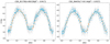 |
Fig. A.1 Fitting results for CSS_J013700.4−081228 and CSS_J044336.7+041144. |
 |
Fig. A.2 Fitting results for CSS_J025611.5+324252 and CSS_J143416.4−173841. |
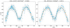 |
Fig. A.3 Fitting results for CSS_J162227.3−063725 and CSS_J095456.8−123840. |
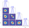 |
Fig. A.4 Posterior distribution of the four parameters for CSS_J162227.3−063725 derived using the proposed method. |
Basic information for the 40 systems from the CSS.
The relative parameters of the 40 systems from the CSS.
The absolute parameters of the 40 systems from the CSS.
References
- Arbutina, B. 2007, MNRAS, 377, 1635 [NASA ADS] [CrossRef] [Google Scholar]
- Cheng, Q., Xiong, J., Ding, X., et al. 2024, AJ, 167, 148 [NASA ADS] [CrossRef] [Google Scholar]
- Christopoulou, P.-E., Lalounta, E., Papageorgiou, A., et al. 2022, MNRAS, 512, 1244 [CrossRef] [Google Scholar]
- Conroy, K. E., Kochoska, A., Hey, D., et al. 2020, ApJS, 250, 34 [Google Scholar]
- D’Angelo, C., van Kerkwijk, M. H., & Rucinski, S. M. 2006, AJ, 132, 650 [CrossRef] [Google Scholar]
- Drake, A. J., Djorgovski, S. G., Mahabal, A., et al. 2009, ApJ, 696, 870 [Google Scholar]
- Drake, A. J., Catelan, M., Djorgovski, S. G., et al. 2013, ApJ, 763, 32 [NASA ADS] [CrossRef] [Google Scholar]
- Drake, A. J., Graham, M. J., Djorgovski, S. G., et al. 2014, ApJS, 213, 9 [Google Scholar]
- Gaia Collaboration (Vallenari, A., et al.) 2023, A&A, 674, Al [NASA ADS] [Google Scholar]
- Green, G. M., Schlafly, E., Zucker, C., Speagle, J. S., & Finkbeiner, D. 2019, ApJ, 887, 93 [NASA ADS] [CrossRef] [Google Scholar]
- Hoffman, M. D., Gelman, A., et al. 2014, J. Mach. Learn. Res., 15, 1593 [Google Scholar]
- Huang, S.-S. 1966, ARA&A, 4, 35 [NASA ADS] [CrossRef] [Google Scholar]
- Hut, P. 1980, A&A, 92, 167 [NASA ADS] [Google Scholar]
- Kochanek, C. S., Adams, S. M., & Belczynski, K. 2014, MNRAS, 443, 1319 [NASA ADS] [CrossRef] [Google Scholar]
- Kopal, Z. 1959, Close Binary Systems (Chapman & Hall) [Google Scholar]
- Lalounta, E., Christopoulou, P.-E., Papageorgiou, A., Ferreira Lopes, C. E., & Catelan, M. 2024, AJ, 168, 50 [NASA ADS] [CrossRef] [Google Scholar]
- Landin, N. R., Mendes, L. T. S., & Vaz, L. P. R. 2009, A&A, 494, 209 [NASA ADS] [CrossRef] [EDP Sciences] [Google Scholar]
- Li, L., & Zhang, F. 2006, MNRAS, 369, 2001 [CrossRef] [Google Scholar]
- Li, K., Gao, X., Liu, X.-Y., et al. 2022, AJ, 164, 202 [NASA ADS] [CrossRef] [Google Scholar]
- Liu, X.-Y., Li, K., Michel, R., et al. 2023, MNRAS, 519, 5760 [CrossRef] [Google Scholar]
- Lucy, L. B., & Wilson, R. E. 1979, ApJ, 231, 502 [NASA ADS] [CrossRef] [Google Scholar]
- Maceroni, C., & van’t Veer, F. 1996, A&A, 311, 523 [NASA ADS] [Google Scholar]
- McCarthy, P. J., Kapahi, V. K., van Breugel, W., et al. 1996, ApJS, 107, 19 [NASA ADS] [CrossRef] [Google Scholar]
- Nair, V., & Hinton, G. E. 2010, in Proceedings of the 27th International Conference on Machine Learning (ICML-10) (Haifa, Israel: Omnipress), 807 [Google Scholar]
- Nandez, J. L. A., Ivanova, N., & Lombardi, J. C., J. 2014, ApJ, 786, 39 [NASA ADS] [CrossRef] [Google Scholar]
- Panchal, A., & Joshi, Y. C. 2021, AJ, 161, 221 [NASA ADS] [CrossRef] [Google Scholar]
- Papageorgiou, A., Christopoulou, P.-E., Ferreira Lopes, C. E., et al. 2023, AJ, 165, 80 [NASA ADS] [CrossRef] [Google Scholar]
- Pecaut, M. J., & Mamajek, E. E. 2013, ApJS, 208, 9 [Google Scholar]
- Pešta, M., & Pejcha, O. 2023, A&A, 672, A176 [NASA ADS] [CrossRef] [EDP Sciences] [Google Scholar]
- Pojmanski, G. 1997, Acta Astron., 47, 467 [Google Scholar]
- Poro, A., Sarabi, S., Zamanpour, S., et al. 2022, MNRAS, 510, 5315 [NASA ADS] [CrossRef] [Google Scholar]
- Poro, A., Hedayatjoo, M., Nastaran, M., et al. 2024, New A, 110, 102227 [NASA ADS] [CrossRef] [Google Scholar]
- Prša, A., & Zwitter, T. 2005, ApJ, 628, 426 [Google Scholar]
- Prša, A., Conroy, K. E., Horvat, M., et al. 2016, ApJS, 227, 29 [Google Scholar]
- Qian, S. 2003, MNRAS, 342, 1260 [CrossRef] [Google Scholar]
- Qian, S. B., Yang, Y. G., Soonthornthum, B., et al. 2005, AJ, 130, 224 [NASA ADS] [CrossRef] [Google Scholar]
- Qian, S., Yang, Y., Zhu, L., He, J., & Yuan, J. 2006, Ap&SS, 304, 25 [NASA ADS] [CrossRef] [Google Scholar]
- Rasio, F. A. 1995, ApJ, 444, L41 [NASA ADS] [CrossRef] [Google Scholar]
- Ricker, G. R., Winn, J. N., Vanderspek, R., et al. 2015, J. Astron. Telesc. Instrum. Syst., 1, 014003 [Google Scholar]
- Stepien, K. 2011, A&A, 531, A18 [NASA ADS] [CrossRef] [EDP Sciences] [Google Scholar]
- Sun, W., Chen, X., Deng, L., & de Grijs, R. 2020, ApJS, 247, 50 [NASA ADS] [CrossRef] [Google Scholar]
- Torres, G. 2010, AJ, 140, 1158 [Google Scholar]
- Tylenda, R., Hajduk, M., Kaminski, T., et al. 2011, A&A, 528, A114 [NASA ADS] [CrossRef] [EDP Sciences] [Google Scholar]
- Vilhu, O. 1982, A&A, 109, 17 [NASA ADS] [Google Scholar]
- Wang, J., Ding, X., Li, J., et al. 2024, ApJS, 273, 31 [NASA ADS] [CrossRef] [Google Scholar]
- Yang, Y.-G., & Qian, S.-B. 2015, AJ, 150, 69 [NASA ADS] [CrossRef] [Google Scholar]
All Tables
All Figures
|
Fig. 1 Neural network architecture used in this study. The input layer is (n, 5), with n as 150 000 training samples and 5 input parameters: T1, i, q., f, and T2/T1. The output layer is (n, 100), representing the synthetic light curve with 100 phase points. The hidden layers contain 50, 500, and 200 nodes, respectively. The Relu activation function (Nair & Hinton 2010) introduces nonlinearity to the model. |
| In the text | |
|
Fig. 2 Comparison between the synthetic light curves generated by the neural network model and those produced by PHOEBE is presented. The upper panel shows the light curve generated by PHOEBE (blue line) and the one produced by the neural network model (orange line). The lower panel presents the residuals between the two curves (blue), with the red dashed line indicating the zero reference. |
| In the text | |
|
Fig. 3 Fitting results for CSS_J042157.5−001751 and CSS_J024234.7+054412 are shown. The blue dots and gray lines represent the observed light curves with photometric errors, while the orange lines depict the light curves generated using the estimated parameters input into the PHOEBE software. |
| In the text | |
|
Fig. 4 Posterior distribution of the four parameters (i, q, f, and T2/T1) for CSS_J042157.5−001751 derived using the proposed method. In each diagonal panel the solid vertical line represents the median (50th percentile) of the parameter distribution. The dashed lines indicate the 68% credible interval, while the dotted lines mark the 95% credible interval. These intervals are also reflected in the off-diagonal contour plots, with the corresponding statistical values provided above the diagonal panels, helping to determine parameter uncertainties. |
| In the text | |
|
Fig. 5 Comparison of the four parameters (i, q, f, and T2/T1). The blue dots correspond to 30 systems from Christopoulou et al. (2022), and the red dots to 9 systems from Lalounta et al. (2024). The orange dashed line represents the 45 degree line. |
| In the text | |
|
Fig. 6 Variation in Js/Jo with q for 40 systems. The orange points illustrate the Js/Jo values for the 40 low mass-ratio contact binary systems identified in this study, while the blue points represent the 30 systems reported by Christopoulou et al. (2022), and the red points correspond to the 9 systems discovered by Lalounta et al. (2024). The gray dashed line marks the instability threshold at Js/Jo = 1/3. |
| In the text | |
|
Fig. A.1 Fitting results for CSS_J013700.4−081228 and CSS_J044336.7+041144. |
| In the text | |
|
Fig. A.2 Fitting results for CSS_J025611.5+324252 and CSS_J143416.4−173841. |
| In the text | |
|
Fig. A.3 Fitting results for CSS_J162227.3−063725 and CSS_J095456.8−123840. |
| In the text | |
|
Fig. A.4 Posterior distribution of the four parameters for CSS_J162227.3−063725 derived using the proposed method. |
| In the text | |
Current usage metrics show cumulative count of Article Views (full-text article views including HTML views, PDF and ePub downloads, according to the available data) and Abstracts Views on Vision4Press platform.
Data correspond to usage on the plateform after 2015. The current usage metrics is available 48-96 hours after online publication and is updated daily on week days.
Initial download of the metrics may take a while.