| Issue |
A&A
Volume 693, January 2025
|
|
|---|---|---|
| Article Number | A33 | |
| Number of page(s) | 18 | |
| Section | Cosmology (including clusters of galaxies) | |
| DOI | https://doi.org/10.1051/0004-6361/202451969 | |
| Published online | 23 December 2024 | |
Mass and light in galaxy clusters: The case of Abell 370
1
Aix Marseille Univ., CNRS, CNES, LAM, Marseille, France
2
Institute of Physics, Laboratory of Astrophysics, Ecole Polytechnique Fédérale de Lausanne (EPFL), Observatoire de Sauverny, 1290 Versoix, Switzerland
3
ESO, Alonso de Córdova 3107, Vitacura, Santiago, Chile
4
LPNHE, CNRS/IN2P3, Sorbonne Université, Université Paris Cité, Laboratoire de Physique Nucléaire et de Hautes Energies, 75005 Paris, France
5
Instituto de Fisica de Cantabria (CSIC-UC), Avda. Los Castros s/n, E-39005 Santander, Spain
6
Centre for Extragalactic Astronomy, Department of Physics, Durham University, Durham DH1 3LE, UK
7
Institute for Computational Cosmology, Durham University, South Road, Durham DH1 3LE, UK
8
Astrophysics Research Centre, University of KwaZulu-Natal, Westville Campus, Durban 4041, South Africa
9
School of Mathematics, Statistics & Computer Science, University of KwaZulu-Natal, Westville Campus, Durban 4041, South Africa
10
Space Telescope Science Institute, 3700 San Martin Drive, Baltimore, MD 21218, USA
11
Department of Astronomy, University of Michigan, 1085 S. University Ave, Ann Arbor, MI 48109, USA
12
STAR Institute, Quartier Agora, Allée du Six Août, 19c, B-4000 Liège, Belgium
13
School of Physics and Astronomy, University of Minnesota, Minneapolis, MN 55455, USA
14
Université Lyon 1, CNRS, Centre de Recherche Astrophysique de Lyon (CRAL), Saint-Genis-Laval, France
15
Physics Department, Ben-Gurion University of the Negev, PO Box 653 Be’er-Sheva 84105, Israel
16
Caltech/IPAC, 1200 E. California Blvd, Pasadena, CA 91125, USA
17
Department of Astronomy/Steward Observatory, University of Arizona, 933 N. Cherry Avenue, Tucson, AZ 85721, USA
18
Department of Astronomy, Yale University, PO Box 208101 New Haven CT 06520, USA
19
Department of Physics, Yale University, PO Box 208120 New Haven, CT 06520, USA
20
Department of Physics and Astronomy, University of California, Los Angeles, CA 90095-1547, USA
⋆ Corresponding author; This email address is being protected from spambots. You need JavaScript enabled to view it.
Received:
23
August
2024
Accepted:
25
October
2024
Abstract
In the cold dark matter (CDM) paradigm, an association between the hypothetic dark matter (DM) and its stellar counterpart is expected. However, parametric strong-lensing studies of galaxy clusters often display misleading features: DM components on the group or cluster scale without any stellar counterpart, offsets between the two components that are larger than what might be allowed by CDM or self-interacting DM models, or significant unexplained external shear components. This is the case in the galaxy cluster Abell 370, whose mass distribution has been the subject of several studies that were motivated by a wealth of data. The cluster was described parametrically with strong-lensing techniques by a model with four dark matter clumps and galaxy-scale perturbers, and with a significant external shear component, whose physical origin remains a challenge. The dark matter distribution features a mass clump without a stellar counterpart and a significant offset between one of the dark matter clumps and its associated stellar counterpart. This paper is based on BUFFALO data, and we begin by revisiting this mass model. Sampling this complex parameter space with Markov chain Monte Carlo (MCMC) techniques, we find a solution that does not require any external shear and provides a slightly better root mean square (RMS) than previous models (0.7″ compared to 0.9″). Investigating this new solution further, in particular, by varying the parameters that lead the MCMC sampler, we present a class of models that can accurately reproduce the strong-lensing data, but whose parameters for the dark matter component are poorly constrained. This limits any insights into its properties. We then developed a model in which each large-scale dark matter component must be associated with a stellar counterpart. This model with three dark matter clumps cannot reproduce the observational constraints with an RMS smaller than 2.3″, and the parameters describing this dark matter component remain poorly constrained. Examining the total projected mass maps, we find a good agreement between the total mass and the stellar distribution, which are both bimodal to first order. We interpret the misleading features of the mass model with four dark matter clumps and the failure of the mass model with three dark matter clumps as being symptomatic of the lacking realism of a parametric description of the dark matter distribution in such a complex merging cluster. We encourage caution and attention on the outputs of parametric strong-lensing modelling. We briefly discuss the implications of our results for using Abell 370 as a gravitational telescope. With the class of models that reproduce the strong- lensing data, we computed the magnifications for background Lyα emitters, and we present the critical curves obtained for the redshift of the Dragon arc, whose recent observations with the James Webb Space Telescope prompted interest. Finally, in light of our results, we discuss the strategy of choosing merging (multi-modal) clusters as gravitational telescopes compared to simple (unimodal) clusters.
Key words: dark matter / large-scale structure of Universe
Based on observations obtained with the Hubble Space Telescope.
© The Authors 2024
 Open Access article, published by EDP Sciences, under the terms of the Creative Commons Attribution License (https://creativecommons.org/licenses/by/4.0), which permits unrestricted use, distribution, and reproduction in any medium, provided the original work is properly cited.
This article is published in open access under the Subscribe to Open model. This email address is being protected from spambots. You need JavaScript enabled to view it. to support open access publication.
1. Introduction
Observations and numerical simulations both support the association between mass and light at the galaxy cluster scale. We refer to mass as the largely dominating dark matter (DM) component whose existence remains to be confirmed. We refer to light as the associated stellar component, which in most cases is in the form of the brightest cluster galaxy (BCG). Observationally, no cluster-scale DM clump without any associated light concentration has been reliably detected so far. In addition, stars in hydrodynamical simulations form in the potential well of DM haloes. This results in the hierarchical formation of a bright galaxy at the centre of the underlying DM halo.
If DM is collisionless, as proposed in the cold dark matter (CDM) scenario, the association between mass and light should be perfect, that is, the offset between the peaks of each component should be equal to zero (Roche et al. 2024). If DM is self-interacting, this offset is possible and should be of the order of a few dozen kiloparsec at most, according to simulations (Kim et al. 2017; Robertson et al. 2017; Tulin & Yu 2018; Fischer et al. 2021; Adhikari et al. 2022).
The observation of offsets between DM and light would therefore be an interesting probe of the DM properties, in particular, its possible self-interaction. Since DM is more likely to interact in colliding clusters than in relaxed clusters, offsets are more likely to be found in merging clusters. DM should experience a drag force (similar to the one experienced by the X-ray emitting gas, but with a much smaller amplitude) that does not affect the stellar component, and will therefore cause a separation between the stellar and the DM components. This configuration has recently been studied numerically by quantifying this offset for different values of the self-interaction cross section of DM particles (Sirks et al. 2024). For a vanishing cross section (corresponding to the CDM case), a spatial offset consistent with zero was retrieved. For cross sections equal to 0.1 and 1 cm2/g, a mean offset of 5 and 12 kpc, respectively, was derived by these authors. This is the same order of magnitude as was found in recent El Gordo-like simulations by Valdarnini (2024): 28 kpc, with a cross section equal to 1 cm2/g.
Observationally, no such offset has been reliably detected so far. In practice, we need to be able to constrain the position of the peak of the DM component with sufficient accuracy, that is, smaller than the typical offset we aim to detect. Gravitational lensing is a useful method in this respect. The typical positional uncertainty of weak gravitational lensing is still ∼10″ (which translates into ∼45 kpc for a cluster at redshift 0.3) using the currently available data (Kim et al. 2017, 2021). Strong lensing (SL) is much more promising in this respect. The current typical uncertainties are at the sub-arcsec level. However, multiple image misidentification can complicate the situation (see the works by Massey et al. 2015, 2018, in Abell 3827), together with the assumed lens properties (see Lin et al. 2023, in Abell 3827).
In the case of the merging Bullet cluster, where the positions of the DM clump are well constrained by SL, no such offset has been detected. This provides an upper limit on the self- interacting cross section of DM equal to 1.25 cm2/g (Randall et al. 2008). The non-detection of this offset in a sample of 72 colliding clusters by Harvey et al. (2015) led to an upper limit equal to 0.47 cm2/g.
Beyond the offset between a DM clump and its associated stellar component is the notion of a dark clump, that is, a group- or cluster-scale DM clump without an associated luminous counterpart. As mentioned earlier, a dark clump has never been reliably detected so far, but these features are seen in parametric SL mass modelling of clusters, both unimodal and multi-modal. The physical interpretation of these dark clumps can be misleading and limits the advantages of parametric SL modelling, which are that the description of the mass clumps can be inferred through a SL analysis and compared with the theoretical expectations. We therefore consider it worthwhile to study the details of SL mass models for which these misleading features are reported. In Limousin et al. (2022, L22 hereafter), we revisited three parametric mass models for which previous (sometimes independent) analyses displayed dark clumps. The three clusters in that study were AS 1063, MACS J0416, and MACS J1206. We presented competitive mass models that did not require the inclusion of dark clumps. We proposed a working hypothesis in which each DM clump should coincide with the associated stellar component within a few dozen kiloparsec, which is the typical offset allowed by SIDM models.
Following this approach, we revisit the mass model of Abell 370 here, for which parametric studies suggest the presence of DM that is not associated with light. Our aim is to determine whether we can propose a mass model in which the DM component is traced by light.
We begin by reviewing the parametric mass modelling that was performed on Abell 370 in Sect. 2, and we revisit the current mass model with four DM clumps in Sects. 3 and 4. We then propose a mass model with three DM clumps in which mass is traced by light in Sect. 5. We discuss our results and conclude in Sect. 6, and we briefly present the implication of our findings for high-redshift studies in Sect. 7.
2. Mass and light in Abell 370
Abell 370, a rich galaxy cluster located at z = 0.375, is of historical relevance when it comes to strong lensing, since in this cluster, the first giant gravitational arc was discovered (Lynds & Petrosian 1986; Soucail et al. 1987; Lynds & Petrosian 1989). A first look at an optical image of the core of Abell 370 reveals a complex light distribution that suggests a complex underlying mass distribution (see Fig. 1, as well as the smoothed light map presented in Lagattuta et al. 2017) caused by an ongoing merger (Molnar et al. 2020).
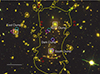 |
Fig. 1. Core of Abell 370 from BUFFALO data (F814/F606/F435 filters). The cyan circles correspond to the location of the four DM clumps from N23, and the magenta circles show their locations from model (ii) (Sect. 3.5). We draw in yellow the critical curve for z = 2 generated from model (ii). The white squares show the location of each clump in the mass model with three DM clumps (Sect. 5). The green ellipses show the cluster members that were optimised individually. We show in red the Lyman-α emitters from Claeyssens et al. (2022), for which we computed a magnification (Sect. 7). North is up, and east is left. The horizontal bar represents 20″, which corresponds to ∼100 kpc at the redshift of Abell 370. |
The light distribution is dominated by the light associated with two dominant bright galaxies, which we refer to as the northern and southern BCG (BCG-N and BCG-S hereafter). We also observe a crown of bright galaxies that surrounds BCG-N, a light concentration in the east (east component hereafter), as well as another one farther north.
Parametric mass models based on the observation of multiple images have been proposed in the past. We review those that are most relevant for this work, in particular, for the description of the smooth dark matter distribution. As is usually done, cluster members are added to this smooth component, using scaling laws to relate their total mass to their luminosity (see, e.g. Limousin et al. 2007).
Advanced Camera Survey multi-band images were obtained as part of the Early Release Observation that followed the Hubble Service Mission 4. Based on these data, Richard et al. (2010), reported nine multiply imaged systems. Describing the cluster with a bimodal mass distribution, that is, two DM clumps associated with each BCG, they were able to reproduce the multiple images with an RMS equal to 1.76″. The northern DM clump was found to be located at ∼10″ from BCG-N.
Richard et al. (2014) analysed new WFC3 data and reported 12 systems. The description of the mass distribution remained bimodal. The SL optimisation was performed in the source plane. This mass model was constructed in light of the forthcoming Hubble Frontier Fields (HFF) data.
The wealth of new constraints revealed by the depth of the HFF data motivated several groups to propose new mass models. In particular, Lagattuta et al. (2017) proposed a mass model that compared to pre-HFF data included two additional DM haloes. This resulted in a mass model with four DM clumps. One of them is associated with BCG-S, one with BCG-N, and one with the eastern light component. The fourth clump is not associated with any light concentration and ends up between BCG-S and BCG-N. It is called “the bridge”. As in Richard et al. (2010), the DM clump associated with BCG-N lies at ∼10″ from BCG-N. They reported an RMS equal to 0.94″.
Additional data obtained with MUSE provided more constraints, and the number of spectroscopically confirmed images doubled. The mass model was revisited by Lagattuta et al. (2019, L19 hereafter). It still consisted of four large-scale DM clumps. They also individually optimised a few cluster members: BCG-S and BCG-N, as well as four cluster members (green circles in Fig. 1) that are located close to multiple images and that are important for reproducing their observed positions accurately. The authors also introduced a strong external shear component (with an amplitude of about 0.1) in order to lower the RMS. They failed to find a physical origin for this external shear component. They also tried to add another DM clump associated with the light distribution located farther north, but its velocity dispersion converged towards zero, suggesting that it is not required.
Niemiec et al. (2023, N23 hereafter), used BUFFALO (Steinhardt et al. 2020) data in order to pursue a combined strong- and weak-lensing analysis of Abell 370. On the SL side, the main difference between N23 and L19 are small changes in the multiple image and cluster member catalogues. N23 considered the gold BUFFALO catalog of multiple images (the best, most confident, multiply imaged systems, with a very low positional uncertainty and definite spectroscopic detection), as well as the BUFFALO cluster members catalogue. The description of the mass distribution and the number of optimised components was the same as in L19. They reported an RMS equal to 0.90″. Using WL, they detected substructures in the outskirts. The inclusion of these substructures in the outskirts did not help them to explain the external shear component, which remained in their model. Using extensive spectroscopic data covering the BUFFALO field of view, Lagattuta et al. (2022) also failed to find any clear origin for this shear component, and we question this in this work.
Recently, Gledhill et al. (2024) reported an updated model using JWST data. They reported no new spectroscopically confirmed multiply imaged systems and found that the overall shape of the critical curve is similar to previous models. Their parametric model features five large-scale DM haloes whose positions are not given in the paper.
More recently, Li et al. (2024) proposed a new mass model in order to study the transient events detected in the giant arc in the new JWST data. They first constructed a preliminary lens model using the same set of multiple images as L19. They reported that a mass model composed of two (NFW) large-scale DM haloes (plus individual galaxies) cannot reproduce the multiple images. These observational constraints are well reproduced (RMS equal to 0.88″) by a mass model with three clumps, however, and they reported that including a forth clump provided no improvement, in contrast to what was claimed by L19 and N23. Their model included an external shear component with a much smaller amplitude (0.03) than was required by L19 and N23. The positions of these three NFW DM mass clumps show that none of them is associated with a luminous counterpart. However, since they added the cluster members in their model, the total mass distribution might follow the light distribution, but this information is not given in the paper, which concentrates on the giant arc. Their second NFW mass clump has a concentration parameter equal to 0.28, which never happens in any numerical simulation. At the same time, they also individually optimised the mass associated with both BCGs. If the halo associated with BCG-S has a position coincident with the light peak of the latter, the halo associated with BCG-N has a position that is at 12″ from the light peak of BCG-N, coincident with the position of their third DM halo. They then added multiple images located in the giant arc to improve their model in this area.
To summarise, if parametric mass modelling is able to reproduce the wealth of spectroscopically confirmed multiple images with a good accuracy (RMS < 1″), none of these models fully associates DM with light.
3. Revisiting the mass model with four DM clumps
3.1. Starting point
The starting point of this study is the SL model described in N23 and illustrated in Fig. 1. It reproduces the observational constraints with an RMS equal to 0.90″, which is comparable with that of L19 (0.78″). It has been optimised in the image plane. We use the same sets of multiply imaged systems and cluster members as in N23 throughout. In addition, all models are optimised in the image plane using the LENSTOOL software (Jullo et al. 2007).
3.2. Rerunning the N23 model
We first repeated exactly the same run as was presented in N23 twice, that is, we used the very same LENSTOOL input files (parameter file, cluster members catalogue, and multiple image file). We reached an RMS equal to 0.76″ and 0.80″. The values of the individual parameters describing the DM distribution differed. We return to this issue below.
This model displays significant external shear, with an amplitude of about 0.1, which is comparable to that of N23. To place this in context, this shear amplitude would be experienced at ∼150″ from the centre of the galaxy cluster Abell 1689 (Limousin et al. 2007). When this external shear component is removed from the model, we obtain an RMS equal to 1.01″. We refer to this last model (without external shear) as model (i) in the following.
3.3. Priors on the galaxy-scale component
The degeneracies between the smooth DM component and the galaxy-scale component in SL studies are well known. We refer to Limousin et al. (2016) and L22 for a discussion. By measuring the mass associated with the cluster members, this degeneracy can be broken, as proposed by Bergamini et al. (2019, B19 hereafter) and more recently by Beauchesne et al. (2024).
Using MUSE spectroscopy, B19 were able to provide priors on the scaling laws used in the SL modelling that relate the mass associated with a given cluster member with its luminosity. No similar study is yet available for Abell 370, and we extrapolated the results by B19 to Abell 370. From the sample of three clusters studied by B19, we used the results derived for MACS 0416. Located at z = 0.39, this cluster of the B19 sample is closest in redshift to Abell 370 (z = 0.37). In the B19 sample, the dynamical state of this cluster is also closest to that of Abell 370, that is, it presents a multimodal light and mass distribution.
B19 proposed a Gaussian prior on the velocity dispersion of a mag = 17.05 (F160W) magnitude equal to σ = 248 ± 28 km s−1. We imposed a Gaussian prior equal to 248 ± 50 km s−1, which broadened the error bar in order to account for the differences between each cluster galaxy populations. To be consistent with B19, we modified the galaxy catalogue of N23 and assigned an F160W magnitude to each member galaxy. In the following, we refer to this prior on the galaxy scale component as the spectroscopic prior. In this way, we obtained an RMS equal to 0.86″, which is slightly larger than but similar to the run with broad priors on the galaxy-scale perturbers. A significant external shear component is favoured, equal to 0.1, similar to the previous models discussed above. The values of the individual parameters describing the DM distribution differ. Even though imposing this spectroscopic prior slightly degrades the RMS, we considered it worthwhile to include it since it is physically and observationally motivated.
Following L19 and N23, we also individually optimised four cluster members as well as BCG-N and BCG-S for all models in this paper (green circles on Fig. 1).
3.4. Removing the external shear component
Keeping the spectroscopic prior, we then removed the external shear component in the modelling. We obtained an RMS of 0.70″, finding that the inclusion of an external shear component is not necessary. We refer to this model as model (ii) in the following. Once again, the values of the individual parameters describing the DM distribution differ.
3.5. Comparing models
We recall that the reference model was obtained by rerunning the N23 files, and its RMS is equal to 0.76″ and the external shear is ∼0.1. Then we derived the following models:
Model (i) is the reference model without external shear, with an RMS equal to 1.01″.
Model (ii) is the reference model without external shear including the spectroscopic priors, with an RMS equal to 0.70″. It constitutes the best model we were able to derive in this paper in terms of RMS. Moreover, it does not require a significant external shear component that cannot be physically explained, and it incorporates a physically motivated prior on the galaxy-scale component.
It is interesting to note that model (ii) is contained in model (i). In model (i), the priors on the galaxy-scale component are large enough to contain the spectroscopic priors incorporated in model (ii). Therefore, in model (i), the sampler could have converged towards model (ii), but it did not, although the fit is better. The priors in the L19 and N23 mass models were large enough to find model (ii). This is puzzling and interesting, and motivates further investigations in order to understand the situation better. This is the subject of the next section.
4. Further investigating the mass model with four DM clumps
Motivated by these findings, we decided to further investigate the mass model with four DM clumps. We recall that for the different models investigated above, the values of the individual parameters describing the four DM mass clumps differ. These are indications that the convergence of the Monte Carlo Markov chain (MCMC) sampler needs to be verified.
Dark matter mass clumps are described using a dual pseudo-isothermal elliptical mass distribution (dPIE profile). We refer to Limousin et al. (2005) and Elíasdóttir et al. (2007) for a description of this mass profile and only give a brief overview here. The geometrical parameters are the position, ellipticity, and position angle. The mass profile is then parametrised by a fiducial velocity dispersion, σ, a core radius, rcore, and a scale radius, rs, which are usually fixed to a high value for cluster-scale DM haloes since SL cannot constrain it. Between r = 0 and r = rcore, the mass density is constant. Then, between r = rcore and r = rs, the mass density is isothermal (r−2), then it falls as r−4 beyond rs.
4.1. RATE and Nb
Two key parameters matter for the convergence of the LENSTOOL MCMC sampler (Jullo et al. 2007): the RATE parameter, associated with the burn-in phase, and the number of iterations (Nb), which is associated with the sampling phase.
The burning phase is made of a sequential Monte Carlo process that gradually samples the priors to the posterior by means of a tempered likelihood  , where T is the likelihood temperature. T progressively decreases from infinity to one. Between each Monte Carlo process, T−1 was updated based on the likelihood estimate at that temperature and the hyperparameter of the sampler RATE. The lower the rate, the more slowly the move of the sampler to the high-likelihood areas, and the less prone it is to missing a mode of the posterior. The larger Nb, the larger the number of iterations of the MCMC chains, and the better the sampling of the parameter space. It is good practice to lower the RATE and to increase Nb until the results obtained on the parameters are stable, in the sense that they remain consistent with each other. This suggests that the runs are not biased by the sampler hyperparameters. The problem is that lowering the RATE and increasing Nb can become computationally very expensive, and this limits our ability to thoroughly investigate the parameter space in an acceptable amount of time.
The N23 mass model was run with a RATE equal to 0.1 and Nb equal to 200, as were our own models presented in Sect. 2, in particular, model (ii). We therefore investigated model (ii) further by lowering the RATE and increasing Nb as long as we could afford it. In practice, we required a run to last three weeks at most on a dedicated modern machine with 12−24 cores.
We show in Table 1 the values of RATE and Nb we investigated, and the corresponding RMS. Two runs had the same RATE, Nb, and RMS (0.7″). However, the parameters differ, as shown in Figs. A.1 and A.2, where we present the corner plots for the parameters of each of the four mass clumps describing the mass distribution in Abell 370 for the different values of RATE and Nb we investigated. Table 1 shows that the best-fit model in terms of the RMS is not found using the values of RATE and Nb that allowed the most precise sampling, and that the RMS ranged from 0.70″ to 1.37″. It might be expected that the best RMS would be associated with the lower RATE and the larger Nb, but this is not the case here. We argue that this is due to the fact that our parametric description is not adapted to Abell 370. In addition, the parameter space likely has several minima, and we may not be able to properly sample it numerically in order to converge to the global minimum. Figures A.1 and A.2 show that the parameters of the DM clumps are very unstable from one run to the next being significantly different. Considering the variance between each run, we conclude that the constraints are very loose for all parameters. Therefore, we do not present the parameters of the best-fit model in a dedicated table, as is usually done in SL studies. We can split this class of eight mass models into four models for which the RMS is smaller than or equal to 1″, and another four models for which the RMS is larger than 1″. However, we see no trends of the inferred values of the parameters of the mass clumps with respect to this dichotomy.
Results for model (ii).
We also further investigated the reference model by N23 in the same way, lowering the RATE and increasing Nb, to determine how this influences the parameters of the DM clumps. The results are presented in Appendix C. We also present in Appendix B the results of this exercise performed on galaxy cluster AS 1063, which illustrate the behaviour of a run that has converged properly. In short, we find that the results for the parameters that describe AS 1063 are very stable with a decreased RATE and increased Nb, and that the corresponding RMSs are equal.
4.2. Galaxy-scale component
In the case of model (i), where no spectroscopic prior was included, we derived a velocity dispersion of 153 km s−1 (for a magnitude of 17.05), which is half of what was derived in model (ii), where a spectroscopic prior was considered (σ = 307 km s−1, which is at the higher end of what is allowed by the spectroscopic prior). The properties of the individually optimised galaxies, in particular the BCGs, are different from the property we would obtain following the spectroscopic prior. BCG-S and BCG-N have a similar magnitude (17.05 and 16.95, respectively), which would correspond to a velocity dispersion in the range 248 ± 50 km s−1 if we followed the spectroscopic prior. The optimised velocity dispersions are the following: For BCG-S, σ = 190 ± 23 km s−1 (model (ii)) and σ = 144 ± 31 km s−1 (model (i)). For BCG-N, σ = 431 ± 8 km s−1 (model (ii)) and σ = 462 ± 23 km s−1 (model (i)). Therefore, the two BCGs, which display a similar magnitude, have very different optimised velocity dispersions. BCGs in clusters constitute a particular class of galaxies that are not representative of the whole cluster member population and may not follow the same scaling relation. Regardless of whether these BCGs follow the spectroscopic prior, they should have a similar velocity dispersion given their similar magnitude. This shows that when spectroscopically measured velocity dispersions become available for Abell 370, it will be relevant to consider them as additional constraints in the mass model.
4.3. DM and light
The working hypothesis proposed in L22 is clearly not verified in the mass models with four clumps that we discussed here (Fig. 1). Of these four DM clumps, a first clump is associated with the bright cluster galaxy located in the south (BCG-S). The shape and orientation of the historical giant arc farther south clearly indicate that BCG-S dominates the total mass distribution in this area, fully justifying a DM clump sitting there. Then, a second DM clump is associated with the bright cluster galaxy located in the north (BCG-N). Slightly farther north, a long thin arc indicates that BCG-N dominates in this area, justifying the inclusion of a DM clump there. These two mass distributions are dominant in Abell 370, as illustrated by a gravitational arc that is rather straight, located between BCG-S and BCG-N. A third DM clump is located in the eastern part of the cluster, which we can associate with a bright galaxy that is located there (Fig. 1). Then, a fourth DM clump is introduced in between BCG-S and BCG-N, without a luminous association. If the positions of the first and third DM haloes coincide with the associated light distribution, the second halo is located at ∼50 kpc from BCG-N, which is on the higher end of what is allowed by alternative DM models such as SIDM (see L22).
We then studied the total projected mass, the quantity that is constrained by SL. We present in Fig. 2 the maps of the mean mass1 obtained for the four mass models that lead to an RMS smaller than or equal to 1″ (Table 1). As expected, they all agree very well. We note that the mass map associated with the larger RMS (1.04″) deviates from the others (whose RMS is equal to 0.73″ and 0.70″), which are almost indistinguishable from each other.
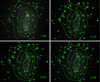 |
Fig. 2. Maps of the mean total projected mass derived from the models leading to an RMS that is smaller than or equal to 1″, as reported on each map. |
4.4. Conclusion on the mass model with four clumps
We conclude that a mass model with four DM clumps is able to accurately reproduce the observational constraints, with an RMS equal to 0.70″. Like previous models (L19 and N23), its DM distribution does not follow the stellar component (Fig. 1, magenta circles). It features a dark clump and a significant offset between DM and light in the north. In addition, we showed that the parameters of each clump as inferred from the different models reproducing the multiple images are poorly constrained. Still, the total projected mass is well constrained by the multiple images, but these multiple images are not able to provide much insight into the properties of DM in Abell 370, such as the number of DM clumps and their properties. As for the external shear that was reported in former studies, we consider that in such a complex and unconstrained parameter space, it is easy to accommodate for an additional component as an external shear. The external shear components included in SL modelling are not always “shear” (Etherington et al. 2024), and different effects inherent to SL modelling can give rise to an effective external shear (see, e.g. Wagner 2019; Lin et al. 2022).
5. Mass model with three DM clumps
Following the working assumption proposed in L22, we investigated a mass model in which each large-scale DM clump is associated with a luminous counterpart. We propose that the total mass distribution in Abell 370 can be described by three DM clumps: one clump that is associated with BCG-S, another clump that is associated with BCG-N, and a final clump that is associated with the bright galaxy located in the east. The position of each clump was allowed to vary in a square of size 6 × 6 arcsec2 centred on the corresponding bright galaxy (Fig. 1), which is typical of what is allowed by SIDM scenarios. We also considered the galaxy-scale perturbers using the spectroscopic priors discussed above. No external shear component was included in the modelling. As before, we investigated different values of RATE and Nb. These values, as well as the corresponding RMS, are shown in Table 2. We present in Fig. A.3 the corner plots for the parameters of each of the three mass clumps describing the DM distribution in Abell 370 for the different values of RATE and Nb we investigated. Because the positions of these mass clumps were forced to be coincident with their luminous counterpart, we do not show theses parameters in the figures for clarity.
Results of the mass model with three clumps.
The best RMS we found, equal to 2.24″, is larger than in the mass model with the four clumps (0.70″). Similar to the behavior seen in the mass model with the four clumps, individual parameters in the model with three clumps are very unstable from one run to the next, and the constraints are very loose. Moreover, an external shear component does not improve a three DM clumps mass model.
Substructures that are located outside the SL area can have an impact on the SL study, as discussed in Acebron et al. (2017). N23 studied in a weak-lensing analysis of the BUFFALO data the surroundings of the core of Abell 370 and detected several substructures. They provided both a grid and a parametric description of these substructures. We tried to take these substructures into account in our SL modelling, but this did not improve the situation, and the parameters of the main DM clumps remain loosely constrained. It is likely that adding more parameters in this already complex and unconstrained parameter space cannot help. We reach the same conclusion in the mass model with four clumps.
Following L22, we included a mild perturbation in the form of a B-spline surface in the lensing potential (Beauchesne et al. 2021) to determine whether this could improve the fit. In contrast to L22, we were unable to find a set of parameters for the B-spline surface that reduced the RMS. To ensure that this was not due to a numerical issue with respect to the complexity of the A370 model, we tried to find such a surface while fixing the parametric model to the best-fit solution, but without more success.
To conclude, a description of the mass distribution with a mass model with three DM clumps whose positions are coincident with the light leads to an RMS larger than 2″. This is three times the RMS that is obtained with a mass model with four DM clumps. Moreover, the parameters of these three clumps are ill defined. The situation is therefore worse than when the RMS is as large as this, but three mass clumps are well defined. We therefore consider that we have failed to describe Abell 370 with a parametric model in which the DM is traced by light.
We compared the maps of the mean total projected mass computed from this mass model with three DM clumps with the map corresponding to our best mass model with four DM clumps (Fig. 3). We find small deviations between these mass maps. We also present the results corresponding to the N23 mass model in this figure. They agree very well with our best-fit mass model.
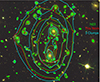 |
Fig. 3. Contours of the mean total projected mass derived from the following models: The mass model with three DM clumps (cyan), the best mass model with four DM clumps (red), and the N23 mass model (green). The contour values are the same for all three models. |
6. Discussion and conclusion
6.1. Comparison with other studies
We compared our results with two other studies that used BUFFALO data: the study using WSLAP+ (Diego et al. 2018), and the study using GRALE (Ghosh et al. 2021). The authors shared their (total) convergence maps (which are proportional to the two-dimensional surface mass density) on the dedicated BUFFALO website. We generated the same quantity from our best-fit model and compare the three maps in Fig. 4.
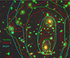 |
Fig. 4. Convergence contours corresponding to the following models: the GRALE model (red), the best model with four DM clumps (green), and the WSLAP+ model (cyan). The contour values are the same for all three models. |
In the south, the three reconstructions agree well, with a peak that is coincident with BCG-S. In the north, our result agrees well with the WSLAP+ result, with a peak that is coincident with BCG-N, while the GRALE reconstruction features a peak that is slightly offset from BCG-N. The eastern component is clearly sub-dominant in the total mass/light budget in all reconstructions. In this region, our reconstruction agrees well with the WSLAP+ result, while the GRALE reconstruction is slightly different.
The WSLAP+ and GRALE methods are both non-parametric, but used different modelling schemes that are described in detail in the corresponding publications. We just report one of the basic differences between the methods to facilitate understanding of the results of the comparison. In GRALE, no assumption is made about a relation between mass and light. In WSLAP+, the surface mass density is described by the combination of a soft component describing the DM and a compact component that accounts for the mass associated with individual cluster galaxies. Therefore, some mass is associated with cluster galaxies by construction. When the smooth DM component alone is considered, then the study by Diego et al. (2018) displays an offset between DM and the associated BCG. This offset disappears when the total mass is considered, which is similar to what we find in this work.
We also compared our results with the result obtained by Cha & Jee (2023) based on HFF data and the non-parametric algorithm MARS. This approach is closer to GRALE than to WSLAP+ since it does not use the galaxy distribution as a prior. In their Fig. 4, the authors report the total mass contours inferred from their analysis. The reconstruction in the south agrees well with the other reconstructions discussed in this section. In the north, their reconstruction displays a mass peak that is offset from BCG-N. This offset is slightly larger than the one found using GRALE.
6.2. Constraints on the DM distribution and interpretation of our results
A mass model with four DM clumps is favoured over a mass model with three DM clumps. The former DM distribution does not follow the stellar component, whereas the latter does by construction. In both cases, the parameters of individual DM clumps are poorly constrained. We showed that in such a complex parameter space, the degeneracies between these parameters are large and little insight into the properties of DM in Abell 370 is gained.
Still, the total projected mass is well constrained and is linked to the stellar component, the two main total mass peaks being coincident with the two BCGs (Fig. 3). We therefore conclude that the total mass is traced by light in Abell 370.
We therefore aim to discuss the underlying DM distribution, which, taken as such, might be misleading. Our questions are about the interpretation of this dark clump, and whether we detect a dark clump. We also determine the interpretation of the offset between the northern DM clump and BCG-N, which is on the higher end of what is allowed by alternative DM models such as SIDM.
These interesting features (the dark clump and the offset) are clearly required by the data in order to reproduce the observed positions of the multiple images with a sub-arcsecond precision. We interpret these as not real, but rather necessary to compensate for the lack of realism in our parametric description of DM clumps during a cluster merging process. We describe the DM component indeed using idealised parametric mass profiles (e.g. dPIE or NFW). This description, though simple, can sometimes be reliable, which is remarkable. In the example of AS 1063 given in Appendix B (a unimodal cluster), the observed positions of the multiple images are well retrieved and the parameters of the DM component are well constrained. In Abell 370, this simple description of the different DM components involved in the merging process might not fully capture the complex underlying physics. Some features such as those reported here are therefore needed to account for the deviations from our idealised parametric descriptions. In L22, we revisited three mass models featuring misleading features in former studies, and we were able to propose competitive mass models that did not require these features. This is not the case for Abell 370. Despite this, we were able to remove the external shear component that was present in former LENSTOOL models. The last parametric study by Li et al. (2024) goes in this direction, in the sense that their DM description contains misleading features, as listed in Sect. 2, that are needed to accurately reproduce the multiple images. Some previous works on Abell 370 reported these features, as summarised in Table 2 by Ghosh et al. (2021).
Even in the JWST era, where hundreds of multiple images are observed, SL mass reconstructions still suffer from degeneracies (Lasko et al. 2023; Liesenborgs et al. 2024), in particular, in merging clusters, and caution and attention should be taken when reading and interpreting the results of any SL model. Furthermore, the authors could discuss the limitations of their models in more detail and help in the understanding and interpretation of their results. We therefore encourage caution and attention on the outputs of parametric SL modelling. This is our main conclusion. We conclude this paper by discussing the implications of our results for using Abell 370 as a gravitational telescope.
7. Implication for high-z studies
The findings of Sect. 4 might have implications for using Abell 370 as a gravitational telescope, since the different models reproducing the SL constraints are likely to provide different magnification estimates for background-lensed objects as well as different critical curves.
7.1. Magnification estimates
Quantifying this effect on global properties such as the luminosity function derived for background objects is clearly beyond the scope of this paper and might be addressed in a forthcoming publication. To illustrate our claim, however, we computed the magnification derived on a few background galaxies. We considered 4 objects selected from the sample of 100 Lyman-α emiters that are lensed by Abell 370 as reported by Claeyssens et al. (2022). Their coordinates and redshifts are given in Table 3, and their locations are shown in Fig. 1. This selection is rather arbitrary; these objects do not have any particular characteristics within the sample. We computed the magnification experienced by these objects using the different mass models investigated in this paper that present an RMS smaller than or equal to 1.0″, that is, those that reproduce the SL constraints with the greatest accuracy. This corresponds to the six models constituting the N23-like class of models (Appendix C), and four models out of the eight models presented in Sect. 3. This makes a total of ten mass models. The results are shown in Fig. 5. The magnification for a given object depends on the mass model that is used, and depending on whether one was to consider a class of models that reproduce the SL constraints instead of one single model, the uncertainties on the magnification estimate would increase. For object 53, we only have five instead of ten curves. For the five mass models that we do not show here, the magnification is unconstrained and has error bars larger than a few hundred. It is therefore not shown for clarity. This is typical of the types of objects that would not be used to study the high-redshift Universe, since the computed magnification values are very unstable. This criterion clearly depends on the mass model considered: depending on the mass model used, one would accept or reject such an object. The uncertainties on the magnification are much larger (sometimes unconstrained) for the mass model with three DM clumps and are not shown.
Lyα emitters.
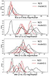 |
Fig. 5. Magnification computed for the four background Lyα-emitters using all models with an RMS smaller than or equal to 1″. |
7.2. Critical curves: Dragon arc
The historical giant arc at z = 0.725, dubbed the Dragon arc, has been the subject of recent interest since JWST observations have led to the discovery of ∼50 microlensed stars in this strongly lensed galaxy (Kelly et al. 2022; Fudamoto et al. 2024). Considering the class of models leading to an RMS smaller than or equal to 1″, we computed the critical curves at z = 0.725 and present them in Fig. 6, together with the location of the microlensing events and the critical curves obtained using WSLAP+. This illustrates the difference in the critical curves from one model to the next. The distribution of microlensing events mostly depends on (i) the position of the critical curve, (ii) the surface mass density of microlenses, (iii) the presence of millilenses (e.g. unresolved globular clusters in the lens plane), and (iv) the bright-end slope of the stellar luminosity function of the background-lensed galaxy (see for instance Diego et al. 2024). Future observations of new transients in this arc will significantly increase the statistics of microlensing events, which will allow us to reverse-engineer the distribution of microlensing events and narrow down the precise location of the macromodel critical curve. This in turn can be used to improve the precision of the lens models in this portion of the cluster.
 |
Fig. 6. Critical curves at z = 0.725 computed for the class of models leading to an RMS smaller than or equal to 1″, both from the N23 class of models (cyan) and from model (ii) in white. In red we plot the critical curves derived with WSLAP+. All these models use the N23 constraints. We show the location of the microlensing events reported by Fudamoto et al. (2024) as white circles and those reported by Kelly et al. (2022) in yellow. |
7.3. Clusters as gravitational telescopes
Related to this issue is the uncertainty on the derived magnification maps in multi-modal clusters such as Abell 370 or MACS 0717 (for which similar conclusions where drawn, see Limousin et al. 2016), and the implications for high-redshift studies in cluster fields. One is tempted to select complex disturbed clusters since they provide a larger area with a high magnification than simple relaxed clusters. This has been the strategy of the Hubble Frontier Fields initiative, where five of the six targets are complex clusters. The problem associated with this approach is that modelling uncertainties do translate into large uncertainties on the magnification estimates, and the area in which the magnification can be considered to be reliable drops significantly (see the discussion by Limousin et al. 2016 in the case of MACS 0717). Therefore, dedicated programs targeting simple clusters might also be considered to build an interesting strategy. The answer cannot be definite, and both populations (complex multi-modal and simple regular clusters) are worth observing, as long as we are aware of the advantages and disadvantages, in particular, as long as we not largely underestimate the errors on the magnifications in the case of complex clusters.
The mean mass map is generated from averaging the individual mass maps computed for each iteration of the MCMC sampler.
Acknowledgments
ML acknowledges the Centre National de la Recherche Scientifique (CNRS) and the Centre National des Etudes Spatiale (CNES) for support. This work was performed using facilities offered by CeSAM (Centre de donnéeS Astrophysique de Marseille). J.M.D. acknowledges the support of project PID2022-138896NB-C51 (MCIU/AEI/MINECO/FEDER, UE) Ministerio de Ciencia, Investigación y Universidades. MJ is supported by the United Kingdom Research and Innovation (UKRI) Future Leaders Fellowship ‘Using Cosmic Beasts to uncover the Nature of Dark Matter’ (grant numbers MR/S017216/1 and MR/X006069/1). AA acknowledges financial support through the Beatriz Galindo program and the project PID2022-138896NB-C51 (MCIU/AEI/MINECO/FEDER, UE), Ministerio de Ciencia, Investigación y Universidades. DJL is partially supported by STFC grants ST/T000244/1 and ST/W002612/1. He is also partially supported by the United Kingdom Research and Innovation (UKRI) Future Leaders Fellowship ‘Using Cosmic Beasts to uncover the Nature of Dark Matter’ (grant number MR/S017216/1). LF acknowledges support by grant No. 2020750 from the United States-Israel Binational Science Foundation (BSF) and grant No. 2109066 from the United States National Science Foundation (NSF), by the Israel Science Foundation Grant No. 864/23, and by the Ministry of Science & Technology, Israel. P.N. acknowledges support from DOE grant #DE-SC0017660. This research was supported by the International Space Science Institute (ISSI) in Bern, through ISSI International Team Project #476 (Cluster Physics From Space To Reveal Dark Matter).
References
- Acebron, A., Jullo, E., Limousin, M., et al. 2017, MNRAS, 470, 1809 [Google Scholar]
- Adhikari, S., Banerjee, A., Boddy, K. K., et al. 2022, ArXiv e-prints [arXiv:2207.10638] [Google Scholar]
- Beauchesne, B., Clément, B., Richard, J., & Kneib, J.-P. 2021, MNRAS, 506, 2002 [NASA ADS] [CrossRef] [Google Scholar]
- Beauchesne, B., Clément, B., Hibon, P., et al. 2024, MNRAS, 527, 3246 [Google Scholar]
- Bergamini, P., Rosati, P., Mercurio, A., et al. 2019, A&A, 631, A130 [NASA ADS] [CrossRef] [EDP Sciences] [Google Scholar]
- Cha, S., & Jee, M. J. 2023, ApJ, 951, 140 [CrossRef] [Google Scholar]
- Claeyssens, A., Richard, J., Blaizot, J., et al. 2022, A&A, 666, A78 [NASA ADS] [CrossRef] [EDP Sciences] [Google Scholar]
- Diego, J. M., Schmidt, K. B., Broadhurst, T., et al. 2018, MNRAS, 473, 4279 [NASA ADS] [CrossRef] [Google Scholar]
- Diego, J. M., Li, S. K., Amruth, A., et al. 2024, A&A, 689, A167 [NASA ADS] [CrossRef] [EDP Sciences] [Google Scholar]
- Elíasdóttir, Á., Limousin, M., Richard, J., et al. 2007, ArXiv e-prints [arXiv:0710.5636] [Google Scholar]
- Etherington, A., Nightingale, J. W., Massey, R., et al. 2024, MNRAS, 531, 3684 [NASA ADS] [CrossRef] [Google Scholar]
- Fischer, M. S., Brüggen, M., Schmidt-Hoberg, K., et al. 2021, MNRAS, 505, 851 [NASA ADS] [CrossRef] [Google Scholar]
- Fudamoto, Y., Sun, F., Diego, J. M., et al. 2024, ArXiv e-prints [arXiv:2404.08045] [Google Scholar]
- Ghosh, A., Williams, L. L. R., Liesenborgs, J., et al. 2021, MNRAS, 506, 6144 [NASA ADS] [CrossRef] [Google Scholar]
- Gledhill, R., Strait, V., Desprez, G., et al. 2024, ApJ, 973, 77 [CrossRef] [Google Scholar]
- Harvey, D., Massey, R., Kitching, T., Taylor, A., & Tittley, E. 2015, Science, 347, 1462 [Google Scholar]
- Jullo, E., Kneib, J.-P., Limousin, M., et al. 2007, New J. Phys., 9, 447 [Google Scholar]
- Kelly, P. L., Chen, W., Alfred, A., et al. 2022, ArXiv e-prints [arXiv:2211.02670] [Google Scholar]
- Kim, S. Y., Peter, A. H. G., & Wittman, D. 2017, MNRAS, 469, 1414 [NASA ADS] [CrossRef] [Google Scholar]
- Kim, J., Jee, M. J., Hughes, J. P., et al. 2021, ApJ, 923, 101 [NASA ADS] [CrossRef] [Google Scholar]
- Lagattuta, D. J., Richard, J., Clément, B., et al. 2017, MNRAS, 469, 3946 [Google Scholar]
- Lagattuta, D. J., Richard, J., Bauer, F. E., et al. 2019, MNRAS, 485, 3738 [NASA ADS] [Google Scholar]
- Lagattuta, D. J., Richard, J., Bauer, F. E., et al. 2022, MNRAS, 514, 497 [NASA ADS] [CrossRef] [Google Scholar]
- Lasko, K., Williams, L. L. R., & Ghosh, A. 2023, MNRAS, 525, 5423 [Google Scholar]
- Li, S. K., Kelly, P. L., Diego, J. M., et al. 2024, ArXiv e-prints [arXiv:2404.08571] [Google Scholar]
- Liesenborgs, J., Perera, D., & Williams, L. L. R. 2024, MNRAS, 529, 1222 [NASA ADS] [CrossRef] [Google Scholar]
- Limousin, M., Kneib, J.-P., & Natarajan, P. 2005, MNRAS, 356, 309 [Google Scholar]
- Limousin, M., Richard, J., Jullo, E., et al. 2007, ApJ, 668, 643 [NASA ADS] [CrossRef] [Google Scholar]
- Limousin, M., Richard, J., Jullo, E., et al. 2016, A&A, 588, A99 [NASA ADS] [CrossRef] [EDP Sciences] [Google Scholar]
- Limousin, M., Beauchesne, B., & Jullo, E. 2022, A&A, 664, A90 [NASA ADS] [CrossRef] [EDP Sciences] [Google Scholar]
- Lin, J., Wagner, J., & Griffiths, R. E. 2022, MNRAS, 517, 1821 [Google Scholar]
- Lin, J., Wagner, J., & Griffiths, R. E. 2023, MNRAS, 526, 2776 [Google Scholar]
- Lynds, R., & Petrosian, V. 1986, BAAS, 18, 1014 [NASA ADS] [Google Scholar]
- Lynds, R., & Petrosian, V. 1989, ApJ, 336, 1 [NASA ADS] [CrossRef] [Google Scholar]
- Massey, R., Williams, L., Smit, R., et al. 2015, MNRAS, 449, 3393 [Google Scholar]
- Massey, R., Harvey, D., Liesenborgs, J., et al. 2018, MNRAS, 477, 669 [NASA ADS] [CrossRef] [Google Scholar]
- Molnar, S. M., Ueda, S., & Umetsu, K. 2020, ApJ, 900, 151 [NASA ADS] [CrossRef] [Google Scholar]
- Niemiec, A., Jauzac, M., Eckert, D., et al. 2023, MNRAS, 524, 2883 [NASA ADS] [CrossRef] [Google Scholar]
- Randall, S. W., Markevitch, M., Clowe, D., Gonzalez, A. H., & Bradač, M. 2008, ApJ, 679, 1173 [NASA ADS] [CrossRef] [Google Scholar]
- Richard, J., Kneib, J., Limousin, M., Edge, A., & Jullo, E. 2010, MNRAS, 402, L44 [NASA ADS] [CrossRef] [Google Scholar]
- Richard, J., Jauzac, M., Limousin, M., et al. 2014, MNRAS, 444, 268 [Google Scholar]
- Robertson, A., Massey, R., & Eke, V. 2017, MNRAS, 467, 4719 [NASA ADS] [CrossRef] [Google Scholar]
- Roche, C., McDonald, M., Borrow, J., et al. 2024, Open J. Astrophys., 7, 65 [Google Scholar]
- Sirks, E. L., Harvey, D., Massey, R., et al. 2024, MNRAS, 530, 3160 [Google Scholar]
- Soucail, G., Fort, B., Mellier, Y., & Picat, J. P. 1987, A&A, 172, L14 [NASA ADS] [Google Scholar]
- Steinhardt, C. L., Jauzac, M., Acebron, A., et al. 2020, ApJS, 247, 64 [Google Scholar]
- Tulin, S., & Yu, H.-B. 2018, Phys. Rep., 730, 1 [Google Scholar]
- Valdarnini, R. 2024, A&A, 684, A102 [NASA ADS] [CrossRef] [EDP Sciences] [Google Scholar]
- Wagner, J. 2019, MNRAS, 487, 4492 [NASA ADS] [CrossRef] [Google Scholar]
Appendix A: Additional figures
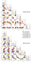 |
Fig. A.1. Corner plots obtained for the parameters of the mass model, for the values of RATE & Nb indicated on the legend. Top: South clump; bottom: north clump. Parameters are significantly different. |
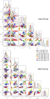 |
Fig. A.2. Corner plots obtained for the parameters of the mass model, for the values of RATE & Nb indicated on the legend. Top: East clump; bottom: dark clump. Parameters are significantly different. |
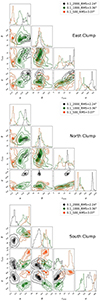 |
Fig. A.3. Corner plots obtained for the parameters of each of the three mass clumps, for the values of RATE & Nb indicated on the legend. Parameters are significantly different. |
Appendix B: AS 1063: Example of a run that has converged
We consider the mass model published in L22, imposing the working hypothesis proposed in this paper (positions of the DM clumps coinciding with the light and ellipticity lower than 0.7) and vary RATE & Nb. Table B.1 shows the results in term of RMS for the different values investigated, and we show in Fig. B.1 the corner plots inferred for each parameter of the mass model, obtained for each value of RATE & Nb. These parameters are the following: position, ellipticity, position angle, core radius and velocity dispersion of the main dominant large-scale DM clump associated with the BCG. Then, we have the scale radius and velocity dispersion of the galaxy scale perturbers (rpot and σpot respectively). We see that the results are very stable, and do not depend on the RATE & Nb: RMS for all runs are similar, and PDFs for all parameters are consistent with each other.
Results on AS 1063.
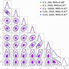 |
Fig. B.1. Corner plots obtained for the parameters of the mass model, for the values of RATE & Nb indicated on the legend. |
Appendix C: Investigating the N23 model further
We consider the mass model proposed by N23, with RATE = 0.1 & Nb = 200, RMS = 0.90″. We then vary RATE & Nb as summarised in Table C.1, where we report the RMS of each run: this constitutes the N23 like class of models. We show in Fig. C.1 and Fig. C.2 the corner plots obtained for each of the four DM clumps parameters.
The best model in terms of RMS is not found for the best values of RATE & Nb, but the RMS values are stable. The corner plots show that the parameters of the DM clumps are very unstable from one run to another, similar to what is found in the investigation of model (ii) exposed in Sect. 3.1.
We then come to the comparison of the total projected mass distributions derived from these models, presenting in Fig. C.3 the results for the N23 and the N23 like class of models, showing a very good agreement between the mass maps. This agreement is expected, given that SL is sensitive to the total projected mass.
N23-like models.
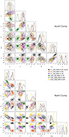 |
Fig. C.1. Corner plots obtained for the parameters of the mass model, for the values of RATE & Nb indicated on the legend. Top: South clump; bottom: north clump. |
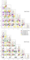 |
Fig. C.2. Corner plots obtained for the parameters of the mass model, for the values of RATE & Nb indicated on the legend. Top: East clump; bottom: dark clump. |
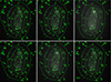 |
Fig. C.3. Maps of the total projected mass derived from the N23 (lower right), and the N23 like class of models. |
All Tables
All Figures
|
Fig. 1. Core of Abell 370 from BUFFALO data (F814/F606/F435 filters). The cyan circles correspond to the location of the four DM clumps from N23, and the magenta circles show their locations from model (ii) (Sect. 3.5). We draw in yellow the critical curve for z = 2 generated from model (ii). The white squares show the location of each clump in the mass model with three DM clumps (Sect. 5). The green ellipses show the cluster members that were optimised individually. We show in red the Lyman-α emitters from Claeyssens et al. (2022), for which we computed a magnification (Sect. 7). North is up, and east is left. The horizontal bar represents 20″, which corresponds to ∼100 kpc at the redshift of Abell 370. |
| In the text | |
|
Fig. 2. Maps of the mean total projected mass derived from the models leading to an RMS that is smaller than or equal to 1″, as reported on each map. |
| In the text | |
|
Fig. 3. Contours of the mean total projected mass derived from the following models: The mass model with three DM clumps (cyan), the best mass model with four DM clumps (red), and the N23 mass model (green). The contour values are the same for all three models. |
| In the text | |
|
Fig. 4. Convergence contours corresponding to the following models: the GRALE model (red), the best model with four DM clumps (green), and the WSLAP+ model (cyan). The contour values are the same for all three models. |
| In the text | |
|
Fig. 5. Magnification computed for the four background Lyα-emitters using all models with an RMS smaller than or equal to 1″. |
| In the text | |
|
Fig. 6. Critical curves at z = 0.725 computed for the class of models leading to an RMS smaller than or equal to 1″, both from the N23 class of models (cyan) and from model (ii) in white. In red we plot the critical curves derived with WSLAP+. All these models use the N23 constraints. We show the location of the microlensing events reported by Fudamoto et al. (2024) as white circles and those reported by Kelly et al. (2022) in yellow. |
| In the text | |
|
Fig. A.1. Corner plots obtained for the parameters of the mass model, for the values of RATE & Nb indicated on the legend. Top: South clump; bottom: north clump. Parameters are significantly different. |
| In the text | |
|
Fig. A.2. Corner plots obtained for the parameters of the mass model, for the values of RATE & Nb indicated on the legend. Top: East clump; bottom: dark clump. Parameters are significantly different. |
| In the text | |
|
Fig. A.3. Corner plots obtained for the parameters of each of the three mass clumps, for the values of RATE & Nb indicated on the legend. Parameters are significantly different. |
| In the text | |
|
Fig. B.1. Corner plots obtained for the parameters of the mass model, for the values of RATE & Nb indicated on the legend. |
| In the text | |
|
Fig. C.1. Corner plots obtained for the parameters of the mass model, for the values of RATE & Nb indicated on the legend. Top: South clump; bottom: north clump. |
| In the text | |
|
Fig. C.2. Corner plots obtained for the parameters of the mass model, for the values of RATE & Nb indicated on the legend. Top: East clump; bottom: dark clump. |
| In the text | |
|
Fig. C.3. Maps of the total projected mass derived from the N23 (lower right), and the N23 like class of models. |
| In the text | |
Current usage metrics show cumulative count of Article Views (full-text article views including HTML views, PDF and ePub downloads, according to the available data) and Abstracts Views on Vision4Press platform.
Data correspond to usage on the plateform after 2015. The current usage metrics is available 48-96 hours after online publication and is updated daily on week days.
Initial download of the metrics may take a while.