| Issue |
A&A
Volume 693, January 2025
|
|
|---|---|---|
| Article Number | A284 | |
| Number of page(s) | 17 | |
| Section | Interstellar and circumstellar matter | |
| DOI | https://doi.org/10.1051/0004-6361/202451440 | |
| Published online | 24 January 2025 | |
The coherent magnetic field of the Milky Way halo, the Local Bubble, and the Fan region
1
Université Libre de Bruxelles,
CP225 Boulevard du Triomphe,
1050
Brussels,
Belgium
2
Université de Paris Cité, CNRS, Astroparticule et Cosmologie,
75013
Paris,
France
★ Corresponding author; This email address is being protected from spambots. You need JavaScript enabled to view it.
Received:
9
July
2024
Accepted:
1
November
2024
Abstract
Context. A recent catalogue of the Faraday rotation measures (RMs) of extragalactic sources, together with the synchrotron polarisation data from WMAP and Planck, provide us with a wealth of information on the magnetic fields of the Galaxy. However, the integral character of these observables, together with our position inside the Galaxy, make the inference of the coherent Galactic magnetic field (GMF) complicated and ambiguous.
Aims. We combine several phenomenological components of the GMF – the spiral arms, the toroidal halo, the X-shaped field, and the field of the Local Bubble – to construct a new model of the regular GMF outside the thin disc.
Methods. We use the binned χ2 approach to fit the parameters of the model to the data. To have control over the relative contributions of the RM and polarisation data to the fit, we pay special attention to the estimation of errors in data bins. To this end, we developed a systematic method that is uniformly applicable to different data sets. This method takes into account individual measurement errors, the variance in the bin, and fluctuations in the data at angular scales that are larger than the bin size. This leads to a decrease in the errors and, as a result, to better sensitivity of the data to the model content. We cross checked the stability of our method with the new LOFAR data, which have very small errors on the measurements of individual sources.
Results. We find that the four components listed above are sufficient to fit both the RM and polarisation data over the whole sky with only a small fraction masked out. Moreover, we have achieved several important improvements compared to previous approaches. Due to our location inside of the Local Bubble, our model does not require the introduction of striated fields. For the first time, we show that the Fan region can be modelled as a Galactic-scale feature. The pitch angle of the magnetic field in our fit converges to a value of around 20 degrees. Interestingly, this value is very close to the direction of the spiral arms inferred recently from Gaia data on upper-main sequence stars.
Key words: cosmic rays / ISM: magnetic fields / galaxies: magnetic fields
© The Authors 2025
 Open Access article, published by EDP Sciences, under the terms of the Creative Commons Attribution License (https://creativecommons.org/licenses/by/4.0), which permits unrestricted use, distribution, and reproduction in any medium, provided the original work is properly cited.
This article is published in open access under the Subscribe to Open model. This email address is being protected from spambots. You need JavaScript enabled to view it. to support open access publication.
1 Introduction
It is well known that our Galaxy is permeated with magnetic field. This field is intricately linked to the evolution of the galaxy, and affects gas dynamics and, in particular, influences star formation and the propagation of cosmic rays, and shapes the Galactic emission at radio frequencies. Accurately accounting for the Galactic magnetic field (GMF) is key to solving the long-standing puzzle of sources of ultra-high-energy cosmic rays (UHECRs). However, the structure, origin, and evolution of the GMF are still not well understood.
In addition to the small-scale turbulent field, radio observations of external galaxies indicate the presence of a large-scale coherent field ordered on scales comparable to the size of the galaxy (Beck 2015). Interestingly, two different and coherent components can be identified. The first component is the magnetic field lying in the plane of the galactic disc and forms so-called magnetic arms, which are not necessarily coincident with the gaseous or optical spiral arms. These spiral magnetic structures are found in almost every spiral galaxy observed so far (e.g. the magnetic arms of M51 (Fletcher et al. 2011) or the disc field of M101 (Berkhuijsen et al. 2016)). The second component, on the contrary, extends out of the disc into the galactic halo and forms an X-shaped pattern, which can be traced up to distances of several kiloparsecs (kpc) away from the galactic plane (e.g. the halo field of NGC 4631 (Mora & Krause 2013) or NGC 5775 (Soida et al. 2011)).
In the standard paradigm, the galactic coherent field is explained as the result of the action of a large-scale dynamo (for a review see Beck et al. 2019 and Brandenburg & Ntormousi 2023), which can also link the coherent field of the disc and the X-shaped field of the halo (Moss & Sokoloff 2008). Alternatively, this coherent field could be the result of gravitational compression of a primordial magnetic field of nanogauss strength that occurred during structure formation (Howard & Kulsrud 1997).
While other galaxies are observed from outside and their global magnetic field structure can be relatively easily recognised, our location inside the Galactic disc makes such measurements for the Milky Way a non-trivial problem. Typically used tracers of magnetic field such as Faraday rotation measures (RMs) of polarised sources or synchrotron emission of cosmic ray electrons (CREs) provide information integrated over the line of sight. Thus, one has to solve the inverse problem of reconstructing the global three-dimensional GMF structure from sky projections of several GMF-sensitive observables. This is not possible without making assumptions regarding the global GMF structure.
The situation is further complicated by the fact that these integral tracers receive contributions from magnetised and ionised bubbles located in the Galactic disc (Wolleben et al. 2010), typically within 100–200 pc from the Galactic plane. Moreover, the Solar System itself is located inside one of these bubbles, which is usually referred to as the Local Bubble (Pelgrims et al. 2020) and is generally believed to be the remnant of a supernova explosion. Several other nearby bubbles seen from the exterior can also be identified. They produce large-scale anomalies in the RM and synchrotron polarisation data at high Galactic latitudes that have to be subtracted or masked. The problem gets worse as more bubbles contribute for the lines of sight closer to the Galactic plane, and appears untractable without invoking distance-sensitive (tomographical) methods. As a result, the information on the global structure of the magnetic field in the disc, particularly in the direction of the Galaxy center, is highly uncertain.
Several phenomenological models of the coherent GMF have been proposed previously, which differ in their complexity as well as the underlying data and fitting techniques used. The first generation of models used synchrotron data and earlier compilations of the RMs of pulsars and extragalactic sources (Han et al. 1997; Tinyakov & Tkachev 2002; Beck 2001). After the arrival of the first all-sky RM catalogue of extragalactic objects (Taylor et al. 2009), the next generation of models included this catalogue as the main data source for reconstruction of the magnetic field in the halo (Pshirkov et al. 2011). The combination of RM and synchrotron polarisation data provides an additional, powerful tool for model building (Jansson & Farrar 2012a). Recent models using various combinations of the existing data include those of Han et al. (2018), Xu & Han (2019), Shaw et al. (2022), Unger & Farrar (2024), and Xu & Han (2024).
The purpose of this paper is to present a new model of the GMF with a focus on the halo field, which we then use to understand the field outside of the thin disc. There are several factors motivating us to update the existing models. On one hand, a significant amount of new RM data has recently appeared. For instance, the S-PASS/ATCA survey of Schnitzeler et al. (2019) filled the blind spot of the RM catalogue of Taylor et al. (2009) used in previous studies. The Wilkinson Microwave Anisotropy Probe (WMAP) synchrotron polarisation data have been updated in Bennett et al. (2013) and more recently in Watts et al. (2023). On the other hand, even the most recent existing models leave a lot of scope for improvement. The model of Pshirkov et al. (2011) did not include the synchrotron polarisation data. The model of Jansson & Farrar (2012a) assumed the magnetic field to be, to some degree, ‘striated’ (flipping direction in random domains), which is a way to boost the synchrotron polarisation signal with respect to the RMs by an arbitrary factor; striation was treated by these authors as a phenomenological parameter. Lastly, but equally important, there is large freedom in choosing and param-eterising the main components of the GMF. Comparing the results of independently constructed fits gives some understanding of the systematic uncertainties involved. While this paper was in preparation, a new model of the GMF was presented by Unger & Farrar (2024); their results and those presented here should be considered complementary in this sense.
In the present paper, we use the WMAP synchrotron polarisation measurements at 23 GHz (Bennett et al. 2013) and the catalogue of about 59 000 RMs of extragalactic sources (Van Eck et al. 2023) to fit the parameters of our model. Even though mostly the same data were used in previous models, including the recent model by Unger & Farrar (2024), we have made several essential improvements.
First, we model and take into account the contribution of the Local Bubble. Its importance was first pointed out by Alves et al. (2018) when considering polarised dust emission observed by Planck at 353 GHz. In previous models that used the RM and synchrotron data together, it was found that the magnetic field that best fitted the RM data alone is insufficient by a factor of 1.5–3 (Unger & Farrar 2024) to explain the observed polarised intensity at high Galactic latitudes. To reconcile the two sets of data, the striation parameter was introduced. Here we show that a sizeable contribution of the Local Bubble to the polarisation signal at 23 GHz solves this ‘synchrotron deficit’ problem, while being fully compatible with the RM data. Using the simplest model of the Local Bubble, we achieved a significant improvement in the quality of the fit, especially at high Galactic latitudes |b| > 60°, thus completely eliminating the need for the striated magnetic fields.
Second, we have developed a uniform approach to the error estimation, which, although technically complicated, is a crucial step in fitting together data of different nature, namely the RM and synchrotron polarisation in our case. We therefore have control of the relative importance of the RM and synchrotron polarisation data in the global fit. The key observation here is that one of the main origins of the ‘noise’ in the data is common in both cases – the magnetised bubbles in the disc. In general, our error bars are smaller than those obtained when using previous methods.
Third, we find from our fit that the pitch angle of the local magnetic arms is 20°. This pitch angle is significantly larger than that found in previous studies, where the pitch angle did not exceed ~10°. This large value is in perfect agreement with the pitch of the Galactic arms inferred from Gaia data by Poggio et al. (2021), as is illustrated below in Fig. 3.
Finally, combining magnetic field in the Local arm with that of the Perseus arm we, for the first time, obtain a good fit of the Fan region – a large bright region on the synchrotron polarisation maps roughly in the direction of the Galactic anti-centre. According to recent studies (Hill et al. 2017), the polarisation signal in this region is produced at 1 – 2 kpc from the Solar System and thus forms part of the global structure (for the model of the Fan region as a local feature, see West et al. 2021). In previous GMF models this region was masked as a local anomaly.
The remainder of the paper is organised as follows. In Sect. 2 we describe the method we use to calculate the error bars on the RM and synchrotron data and discuss the data we used. In Sect. 3 we describe our model for the GMF in the halo. In Sect. 4 we present the results of the global fit of our model to the data. In Sect. 5 we discuss the performance of our model. In particular, in Sect. 5.1 we provide details of the feature introduced in the present model for the first time, namely the Local Bubble. Finally, we sum up our results in Sect. 6. Appendices A and B are devoted to the method of error assignment. In Appendix C1 we compare our results to the previous models.
Throughout the paper and in the numerical code, we fix the coordinate system such that the centre of the Galaxy is at the origin, the z-axis is directed towards the Galactic north pole, and the Solar System coordinates are {−8.2 kpc, 0, 0}. For the observer at Earth, the direction towards positive y is (l, b) = (90°, 0°), and that towards positive ɀ is (l, b) = (0°, 90°).
2 Data preparation
Galactic magnetic field can be probed with different tracers. Among them are polarised thermal emission of dust, Faraday rotation measures of Galactic and extragalactic sources and synchrotron emission of cosmic ray electrons at different frequencies. Each of these tracers is sensitive to different properties of magnetic field but all of them provide us with valuable information about coherent GMF structure. Below, we briefly review each tracer and justify the choice of datasets for our analysis.
Dust. Observations of dust polarised emission reveal the average orientation of the component B⊥ of GMF perpendicular to the line of sight, without providing any information on its strength. The dust is concentrated in the thin disc with the height ~ 100 pc, which means the method is mainly sensitive to our local neighborhood. Significant progress has been achieved thanks to the Planck measurements at a frequency of 353 GHz, where dust emission dominates. Firstly, it was shown that none of the existing models can accurately predict dust emission (Planck Collaboration Int. XLII 2016). Secondly, it was demonstrated that the emission at high Galactic latitudes is dominated by the Local Bubble wall (Skalidis & Pelgrims 2019; Pelgrims et al. 2020). Moreover, it was found that a model where the field in the wall is obtained by compressing an initially uniform field successfully explains the structure of polarisation after fitting the direction of the initial field. We adopted this approach when building our model of the Local Bubble, see Sect. 3.
Rotation measures: Galactic pulsars. Faraday rotation is the phenomenon of rotation of the polarisation plane of a linearly polarised radiowave when propagating through the magnetised plasma. The rotation angle Δθ is proportional to the square of the wavelength λ; the coefficient is called the rotation measure (RM):
 (1)
(1)
where e and me are the electron charge and mass, and the integral is taken along the line of sight between the observer and the source. The RM is proportional to the density of free electrons ne and the component of the magnetic field parallel to the line of sight By,
![Mathematical equation: ${\rm{RM}} \approx 0.812\int_0^l {\left[ {{{{n_e}(s)} \over {{\rm{c}}{{\rm{m}}^{ - 3}}}}} \right]} \left[ {{{{B_}(s)} \over {{{10}^{ - 6}}{\rm{G}}}}} \right]\left[ {{{{\rm{d}}s} \over {{\rm{pc}}}}} \right]{\rm{rad}}/{{\rm{m}}^2}.$](/articles/aa/full_html/2025/01/aa51440-24/aa51440-24-eq2.png) (2)
(2)
Positive RM corresponds to the field pointing towards the observer. Measurement of the polarisation on at least two different wavelengths allows one to calculate RM.
Pulsars are bright sources of polarised radio emission. The advantage of pulsars is their negligibly small intrinsic RM values. Also their location within the galaxy allows for the investigation of the inner structure of the GMF. Study of pulsar RMs gives an indication of the magnetic field reversal in the direction to the Galactic center (Han & Qiao 1994). However, pulsars are mostly concentrated in the disc, which makes them not so useful for studying the GMF halo. Moreover, the distances to pulsars are usually inferred from their dispersion measures, which introduces additional uncertainties. For these reasons we do not use pulsar data in this paper and leave the validation of our model against pulsars for the future.
Extragalactic RM. At the moment more than 59 000 extra-galactic RMs have been measured which are summarised in publicly available master catalogue by Van Eck et al. (2023). In our study we use the latest compilation of this catalog, namely CIRADA consolidated catalogue version v1.2.02. The core of the catalogue is the NRAO VLA Sky Survey (NVSS) survey (Taylor et al. 2009). Additionally, it comprises RMs from Schnitzeler et al. (2019); Van Eck et al. (2021); Betti et al. (2019); Farnes et al. (2014); Mao et al. (2010); Tabara & Inoue (1980); Simard-Normandin et al. (1981); Broten et al. (1988); Riseley et al. (2020); Brown et al. (2003); Taylor et al. (2024); Mao et al. (2012b,a); Feain et al. (2009); Van Eck et al. (2011); Ma et al. (2020); O’Sullivan et al. (2017); Kaczmarek et al. (2017); Anderson et al. (2015); Brown et al. (2007); Klein et al. (2003); Heald et al. (2009); Shanahan et al. (2019); Clarke et al. (2001); Minter & Spangler (1996); Ranchod et al. (2024); Van Eck et al. (2018); Law et al. (2011); Riseley et al. (2018); Livingston et al. (2022); Mao et al. (2008); Roy et al. (2005); Livingston et al. (2021); Oren & Wolfe (1995); Clegg et al. (1992); Kim et al. (2016); Battye et al. (2011); Ma et al. (2019); Rossetti et al. (2008); Costa & Spangler (2018); Vernstrom et al. (2018); Gaensler et al. (2001); Costa et al. (2016), including the most recent extensive Low-Frequency Arrar (LOFAR) survey LoTSS (O’Sullivan et al. 2023) and the Australian Square Kilometre Array Pathfinder survey POSSUM (Vanderwoude et al. 2024).
The totality of extragalactic RMs covers the whole sky almost uniformly with roughly 1 source per 1 deg2 on average, which is very convenient for studying the global structure of the GMF. The smoothed and cleaned RM skymap constructed by Hutschenreuter et al. (2022)3 from the previous version of the catalogue (v0.1.8) is shown in Fig. 1, upper panel. An even earlier version of the catalogue was used for the first time to study magnetic field in the Galactic halo by Pshirkov et al. (2011).
Unlike pulsars, extragalactic sources generally do have intrinsic RMs, which sometimes may be very large, and so the RM data have to be cleaned from these outliers. The exact procedure is described in Appendix A. The bulk of the extragalactic sources have intrinsic RMs with the zero mean and the r.m.s. not exceeding ~7 rad/m2 (Schnitzeler 2010; Pshirkov et al. 2013).
Synchrotron. Relativistic electrons of energy E spiraling in the magnetic field emit radio waves near the critical frequency
![Mathematical equation: ${v_c} \approx 1.6\left[ {{{{B_ \bot }} \over {{{10}^{ - 6}}{\rm{G}}}}} \right]{\left[ {{E \over {10{\rm{GeV}}}}} \right]^2}{\rm{GHz}}.$](/articles/aa/full_html/2025/01/aa51440-24/aa51440-24-eq3.png) (3)
(3)
The resulting synchrotron radiation is polarised in the plane perpendicular to the direction of the magnetic field. Assuming the distribution of cosmic ray electrons (CRE) in energy is known, the information about B⊥ can be extracted from synchrotron measurements. This information is complementary to that contained in RMs.
The CMB experiments WMAP and Planck performed the full-sky synchrotron polarisation measurements with high precision at 23 and 30 GHz, respectively. The WMAP synchrotron skymap was first combined with RM data to study the GMF in Jansson et al. (2009); Sun & Reich (2010); Jansson & Farrar (2012a); Jansson & Farrar (2012b).
At higher frequencies the polarised emission is dominated by the emission from dust. On the other hand, at lower frequencies the Faraday rotation becomes important as can be seen from Eqs. (1) and (3). Significant Faraday rotation leads to depolari-sation of initially polarised beam. The combination of Faraday rotation with the synchrotron measurements at large number of nearby frequencies allows for the so-called Faraday tomography (Burn 1966), when the synchrotron emissivity is determined as a function of RM accumulated along the line of sight. Recently such measurements were performed by GMIMS collaboration in the Northern sky in the frequency band 1280–1750 MHz (Wolleben et al. 2021), and in the Southern sky in the range 300–480 MHz (Wolleben et al. 2019).
In the current study we use the final nine-year WMAP 23 GHz dataset to fit the model. We choose it because firstly, it covers the entire sky, and secondly, it is measured at sufficiently high frequency so that depolarisation is negligible. The use of frequencies at which depolarisation is significant implies an increasingly significant role of local structures which we do not model in this study. On the other hand WMAP 23 GHz and Planck 30 GHz data are very similar after rescaling for the difference in frequency. We could use either one; we choose WMAP because its seven-year version has already been used in Jansson & Farrar (2012a). The residual systematic difference after rescal-ing between WMAP and Planck was studied in detail in the Cosmoglobe project (Watts et al. 2023). We note that this difference is small compared to the current precision of the GMF models, and thus is not important for our purposes. Figure 1 shows the sky maps of Stokes Q and U parameters (middle and bottom panels, respectively) corresponding to the WMAP 23 GHz dataset.
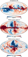 |
Fig. 1 Compilation of the data used in this paper. Upper panel: extra-galactic RM skymap, smoothed and cleaned by Hutschenreuter et al. (2022). We note that in our main analysis, we start with the individual RMs from the CIRADA catalog. The RM skymap from Hutschenreuter et al. (2022) is shown for clearer visual representation. Middle and bottom panels: WMAP synchrotron Stokes Q and U skymaps at 23 GHz (Bennett et al. 2013). |
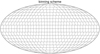 |
Fig. 2 Binning scheme used in this analysis. The bins are rectangular in Galactic coordinates and are arranged in iso-latitude bands of 10° in width. The two equatorial bands are divided into 36 square 10° × 10° bins each. The number of bins in other bands is chosen in such a way as to get the closest approximation to equal-area bins. |
2.1 Binning and error estimation
In order to extract maximum benefit from the combination of the RM and synchrotron polarisation data, we prepare both datasets in a similar way. This includes four steps: removal of outliers, masking, binning and error estimation. The procedures for outliers and masking are different for RMs and synchrotron skymaps and are discussed separately in the Sects. 2.2 and 2.3. On the other hand, for both datasets we adopt the same binning scheme and errors estimation algorithm which are described below.
After getting rid of outliers and applying the masks we are left with a collection of small pixels (or individual RMs) that can be directly used for modelling. However, as we are interested in the coherent part of the GMF it is useful to average the masked RM and synchrotron data over the angular bins of a relatively large size. Indeed, the signal of coherent GMF is expected to vary on scales of tens of degrees, and so bins of a smaller, but not much smaller angular size are sufficient to trace it. Moreover, averaging over large bins effectively cancels small-scale fluctuations in the data and reduces errorbars.
The same approach was already used in previous studies. Pshirkov et al. (2011) and Terral & Ferrière (2017) used the bins with the size ~10°, Jansson & Farrar (2012a); Unger & Farrar (2024), used smaller bins. Since there is no strict criterion for choosing the optimal bin size we use the same bins as Pshirkov et al. (2011) for both RM and synchrotron data, see Fig. 2. The advantage of this binning scheme is that bins form isolatitude bands. The binning scheme was chosen independently of the masks. Those bins where more than 50% of the original content (by area for WMAP and by the number of sources for RM) has been masked were discarded.
After setting the binning scheme the most important step is the estimation of the mean value in each bin and assigning corresponding error bars. Jansson & Farrar (2012a) and Unger & Farrar (2024) used the standard deviation within the bins as an error estimate. We do not see a justification for this choice. If the variations of individual sources (or pixels in the case of polarisation data) from the mean were all independent, the error in the bin should be the standard deviation divided by the square root of the number of sources, typically much smaller than the standard deviation itself. However, bubbles and other structures of large angular size (e.g. Radcliffe Wave (Panopoulou et al. 2024)), which are also part of the noise, make coherent contributions to individual bins, and so the errors should be larger, but likely not as large as the standard deviation. Pshirkov et al. (2011) used a more complex error estimation procedure which for many bins resulted in smaller errors equal to the standard deviation divided by three. Such a procedure, however, lacks a statistical justification and thus is difficult to generalise to the case of two data sets of a different nature.
In this work we propose a new method of error estimation. The observed quantities – RMs or polarised intensity maps – are sums of contributions from the coherent GMF and from fluctuations of different origin, including inhomogeneities of the interstellar medium (ISM), the turbulent component of the GMF, magnetised or ionised clouds, intrinsic RMs of sources, etc., and of different scales including those exceeding the bin size. We do not model such fluctuations and consider them as noise obscuring the coherent GMF signal. Our method to estimate the contribution of this noise to the errors assigned to bins is based on the assumption that its statistical properties only depend on the latitude b. We assess the parameters of the noise at given b by the Fourier analysis of the data in the isolatitude strips, which we then use to estimate the errors.
If the data in a strip only contained noise, then the variance associated with a bin of size L would be given by the sum over modes of the power spectrum with the window function sinc2(kL/2) (see Appendix B for the derivation). We note that this variance includes contributions from scales larger than the bin size. The actual data also contain the coherent part, which is concentrated in the lowest modes and should be subtracted. Moreover, the model that we fit to the data only has sizeable power in the first three harmonics k = 0,1,2, and so we subtract these harmonics before calculating the variance; see Fig. B.1. Specifically, for all bins of the same strip we calculate the variance  according to the formula:
 (4)
(4)
where Sk is the power spectrum of the strip of data to which the bin belongs, and the bin size L is of order 10°. Equation (4) results in errors that are smaller than the simple data variance over the bin by a factor 2–3. We note also that this approach allows us to treat the RM and synchrotron polarisation data on equal footing.
Equation (4) assumes that the mean value in a given bin can be calculated exactly, while in reality this is not the case: the data only sample the underlying function in a number of points, and so the mean calculated from these values has an associated statistical error σµ. We determine this error by fitting the distribution of values in the bin by a Gaussian, which gives both the mean and its statistical error: µ ± σµ. The total error in the bin is thus
 (5)
(5)
For the polarisation data, and for most (but not all) of the RM bins the contribution of σµ is negligible.
We note that the errors σL and σµ have different behaviour when increasing the number of observations N. The error on the mean value of the bin σµ tends to zero approximately as  while σL remains constant.
The details of the calculation of σµ and σL are described in the Appendices A and B, respectively. The procedure is the same for both RM and synchrotron datasets.
2.2 Rotation measure mask
The value of the RM in some directions may be dominated by local features of the ISM. Thus, when fitting the coherent GMF they should be masked out. An illustrative example is the well-known Sh2-27 cloud in the direction (l, b) ≈ (10°, 25°), ionised by the massive star Zeta Ophiuchi passing through it. This cloud is located at the distance of ~100 pc and is clearly visible as a ~10° bright blue spot in the RM map, see Fig. 1. The average RM in the direction of Sh2-27 goes below −100 while RMs in its vicinity are close to zero (Thomson et al. 2019).
Since RM is proportional to the density of thermal electrons, potentially biased regions are expected to correlate with highly ionised nearby bubbles. In order to mask them out it is convenient to use maps of Hα emission. Similar approach was recently used by Unger & Farrar (2024). Using the full-sky Hα map compiled by Finkbeiner (2003) we masked pixels where the intensity of Hα emission is at least twice as strong as the average intensity at the same latitude.
Additionally, based on visual inspection of the RM map from Hutschenreuter et al. (2022) (see Fig. 1) we masked out the arclike segment with positive RMs around (l, b) ≈ (100°, 0° −50°) which is probably related to the Loop III. Also we removed from the analysis bright bubble-like structure at (l, b) ≈ (160°, −15°) and a region with mostly zero RM surrounded by strongly negative RMs near (l, b) ≈ (110°, −10°).
Finally, we excluded the Galactic plane (|b| < 10°) because its modelling depends on the enhancement of thermal electrons density in the spiral arms. Unfortunately, existing models of thermal electrons rely on pre-Gaia measurements of the spiral arms whose pitch was believed to be significantly smaller than that inferred from the Gaia data (Poggio et al. 2021). Our preliminary fits, as well as the final result, favour the same pitch angle as that provided by Gaia, which means these models are incompatible with our setup. The description of the adopted model of thermal electrons is given in Sect. 3.2. The resulting mask is shown in Fig. 6. In total the RM dataset mask covers 26% of the sky.
2.3 Synchrotron mask
The synchrotron mask is built independently of the RM mask. First, we discarded all pixels of the WMAP Stokes Q and U maps marked as corrupted. Then we masked out the brightest, most probably nearby features. Namely, we excluded Loop I and Loop II by cutting out corresponding ring segments. The mask is purely geometrical and manually set to cover the majority of Loop I and Loop II. In contrast with previous studies we do not mask the Galactic plane and the Fan region. We apply this mask for both Stokes Q and U skymaps, see Fig. 6. The mask covers 11% of the sky.
There are many other less prominent loops and spurs visible in the polarisation data apart from the Loop I and Loop II, see Vidal et al. (2015). As these features are not so bright, we do not mask them out in order to keep the mask as small as possible.
3 Model of the Galactic magnetic field
Sky maps of both Faraday rotation and synchrotron polarisation data reveal large regions of constant sign that are aligned with the Galactic plane and the direction to the Galactic center, leaving no doubt of the existence of the coherent magnetic field in the Galaxy. These regions form a particular pattern which has to be reproduced by the magnetic field model. Even though we only measure the projections onto the sky plane of 3-dimensional structures, this requirement turns out to be rather restrictive if one assumes that the model consists of a few simple components. We found that 4 major components are sufficient to describe the global structure of the Faraday rotation and polarisation maps: the thick disc, the toroidal halo, the X-shape halo field and the field of the local bubble. Different parts of the data are more sensitive to different components, but all four are needed for a good global fit. In this section we overview these components and their role in reproducing the key features of the data, and present the results of the global fit.
3.1 Magnetic field components
Thick disc. While most of Galactic stars are concentrated within a couple hundred parsecs from the Galactic plane where they populate the Galactic arms, thermal electrons and coherent magnetic fields are usually assumed to form a larger structure often referred to as the thick disc which generally traces the spiral arms and extends up to 1–2 kpc from the Galactic plane. We assume in this work that the magnetic field associated with this structure is directed along the arms either towards or away from the Galactic center. The solar system is situated at the inner edge of the Local arm; the “local” magnetic field is directed clockwise as viewed from the Galactic North pole, with a pitch towards the center. The detailed structure of the spiral arms in the solar vicinity has been mapped out by Gaia (Poggio et al. 2021) and is discussed further in Sect. 4. There are indications from the pulsar data of the field reversal at ~0.5 kpc in the direction to the Galactic center (Han & Qiao 1994). We therefore assume that the field changes direction to counter-clockwise in the inner Sagittarius-Carina arm.
The typical thickness of the disc is ~1 kpc, which means that only the region within ~6 kpc from the Sun contributes to the observables at Galactic latitudes |b| > 10°. Correspondingly, only the arms that pass in the relative vicinity of the Sun are constrained from our fits to the data. These are, in the first place, the Local and Perseus arms in the outer Galaxy and the Sagittarius-Carina and Scutum arms in the inner Galaxy. Our fits are not sensitive to the field in the Norma and Outer arms. The general shape of the thick disc field is shown in Fig. 3 where the colored region corresponds to distances within 6 kpc from the Sun.
In our model each arm is an independent GMF component. The position of an arm is given by its axis, represented by the logarithmic spiral:
 (6)
(6)
where k = tan or is the tangent of the pitch angle or α, b is an initial phase, and x0 and y0 are the origin of the spiral. The cross section of an arm in the plane perpendicular to its axis is a squircle: the point of the cross section plane belongs to an arm if its coordinates in that plane { , ɀ} satisfy
 (7)
(7)
Here, rdisc and rɀ are two semi-axes of the squircle. The continuous parameter n controls the shape of the cross section. If n = 2 the squircle reduces to an ellipse, while larger n makes it more similar to a rectangle.
The magnetic field of an arm is directed along the arm and varies in inverse proportion to the arm cross section as to guarantee its divergence-free structure. It is parameterised by the value B at the intersection of the arm axis and the line passing through the Sun and the Galactic center. To minimise the number of fitting parameters we take the field to be constant over the arm cross section.
In total each arm is described by 8 parameters: x0, y0, b, α, B, rdisc, rɀ, n. The pitch angles α are taken the same for all arms and are controlled by the common pitch α0 which is allowed to vary freely while fitting. The y-coordinates of the arm origins are zero y0 = 0 for all arms. To the contrary, the x-coordinates xo are individual for each arm and are set by hand to make our magnetic arms better match with the spiral design of the Galaxy. The adjustments of x0 do not affect the result as long as x0 is small compared to the distance from the Sun to the Galactic center. Indeed, in this case the change in x0 is degenerate with the initial phase of the spiral arm b which is a fitting parameter. We make use of this fact to roughly connect major Perseus and Scutum arms with the ends of the Galactic bar. The widths of the arms in the Galactic plane are also set to predefined values close to 1 kpc, see Table 2.
After these adjustments we are left with 4 fitting parameters per arm. For the nearby Local arm and the Sagittarius-Carina arm we fit all 4 parameters, while for the more distant Scutum arm only the strength B.
The Perseus arm is a special case. It contributes to the observables in the direction of the outer Galaxy at low Galactic latitudes where the Fan region is located, which is one of the most prominent features on the synchrotron polarisation maps. In order to fit the Fan region we had to assume that the inner part of the Perseus arm close to the disc has stronger magnetic field as shown in Fig. 4. We assumed for simplicity that the field takes two different constant values across the inner and outer sections of the arm (this can be viewed, of course, as a crude approximation for the field decreasing away from the disc). In total, there are three fitting parameters for the Perseus arm: the field strength B, the additional field in the inner part B′ (so that the total field in this part is B + B′) and the width of the arm rz. The width of the inner part  is fixed to 0.4 kpc. The phase b and shift x0 are chosen in such a way as to make the Perseus and Scutum arms symmetric with respect to the Galactic z-axis: x0(Perseus) = −x0(Scutum), b(Perseus) = b(Scutum) + 180°, see Fig. 4 and Table 2.
Toroidal halo. The field in the thick disc is not sufficient to account for the observed Faraday rotations – a component extending further in the Galactic halo is needed. Previous models have shown the necessity for a toroidal component above and below the Galactic disc with the azimuthal field directions opposite in the North and South. Such a field may arise as a result of the Galactic dynamo (Wielebinski & Krause 1993). This component is schematically shown in Fig. 4.
It has been first noted in Han et al. (1997); Han et al. (1999) and later confirmed by Pshirkov et al. (2011) that the combination of the thick disc and the toroidal halo reproduces well the characteristic all-sky − + − + / − + North/South pattern of the Faraday rotations, provided the directions of the disc field around the Sun location and the toroidal component are opposite in the North and coincident in the South. As a result, the magnetic field in the Galactic Northern sky is somewhat weaker than in the South. If only Faraday rotation data are included, these two components give a reasonable fit to the data (Pshirkov et al. 2011).
We model the toroidal components as cylindrical sections whose axes coincide with the Galactic axis, filled with purely azimuthal magnetic field. Each cylinder is described by 4 parameters: the outer radius rout, lower bound zmin, upper bound zmax and the strength of the field Btor.
X-shape field. When the synchrotron polarisation data are included, we could not fit both RM and synchrotron maps with the thick disc and toroidal halo. With only these two components one cannot reproduce the change of the sign of the Q-parameter around the meridian line 1 = 0, which is particularly visible in the data in the Northern hemisphere, see Fig. 1. As was first noted in Jansson & Farrar (2012a), this can be achieved by adding a second halo component – the X-shape field – in the inner part of the Galaxy. Topologically this field corresponds to the Model C of Ferrière & Terral (2014). Similar fields are observed in some other galaxies viewed edge-on (Beck et al. 2019). To reduce the number of parameters, we take the X-field lines to be symmetric with respect to the Galactic plane, axially symmetric and having everywhere the same inclination angle θ with respect to the Galactic axis. The footprint of the X-field in the disc extends up to rX ~ 6 kpc from the center. The X-field is schematically shown in Fig. 4.
The fitting parameters of the X-field are the strength BX at z = 0, the radius rX of the X-field footprint at z = 0 and the inclination angle θ. The radial profile of the X-field was chosen to be constant. Thus, the footprint of the X-field on a plane above or below the Galactic plane is a ring of inner radius |ɀ|/ cos θ and outer radius |ɀ|/ cos θ + rX. The area of this ring grows with |ɀ|; the strength of the field decreases in inverse proportion so as to keep the field divergence-free.
Local Bubble. The three components described so far reproduce well the overall pattern of both RM and synchrotron data. However, when normalised to the rotation measures, they underestimate the overall strength of the synchrotron polarisation signal at high latitudes by about factor 2. In the previous models of Jansson & Farrar (2012a); Unger & Farrar (2024) where the synchrotron data were included in the fit this problem was solved by introducing the ‘striation’ which allows one to boost the synchrotron polarisation signal relative to the rotation measures. We found that inclusion of the contribution from the Local Bubble may solve the problem without the striation factor.
The Local Bubble is a cavity in the interstellar medium (Lallement et al. 2022) created, presumably, by several local supernova. It is surrounded by clouds of cold dust compressed by hot gas resulted from supernova explosion(s). It has an irregular shape, but in the zeroth approximation can be fitted by an ellipsoid with half-axes of the size of x = 100 pc by y = 200 pc by ɀ = 300 pc (Alves et al. 2018; Pelgrims et al. 2020). The Solar system is located in the inner part of the bubble relatively close to its center.
It turns out that even in a crude approximation of a spherical bubble, the compressed magnetic field on the bubble walls can explain the missing part of the polarisation intensity while having approximately right sky distribution and not spoiling the RM signal. The latter can even be improved by adjusting the parameters of the bubble as discussed in more detail below in Sect. 5.1. This is possible because the polarisation parameters Q and U are quadratic in the field strength, while the RMs are linear.
In our model the bubble is a spherical shell with the inner radius fixed to rLB = 200 pc. While fitting we tuned the thickness of the bubble wall δrLB, the coordinates of the center of the bubble xLB, yLB, zLB, and the direction lLB, bLB of the magnetic field before compression. The field strength in the bubble wall is determined as a result of the compression of magnetic lines of the initially uniform field by the expanding spherically symmetric bubble. We assume that the field outside of the bubble is unperturbed, the field inside is zero, and the field in the wall is tangential to its surface and uniformly distributed across the wall in the radial direction. We also assume that it is symmetric with respect to the axis passing through the center of the bubble and parallel to the original uncompressed field. The field configuration is schematically shown in Fig. 5. Strictly speaking, such field is not divergence-free. However, by adjusting the dependence of the field strength on the distance from the axis one can make it divergence-free at scales larger than the thickness of the wall. The conservation of the magnetic flux at these scales implies the following relation:
![Mathematical equation: ${B_{{\rm{LB}}}}(\theta ) = {B_{{\rm{LB}},0}}\left[ {1 + {{r_{{\rm{LB}}}^2} \over {2{r_{{\rm{LB}}}}\delta {r_{{\rm{LB}}}} + \delta r_{{\rm{LB}}}^2}}} \right]\sin \theta ,$](/articles/aa/full_html/2025/01/aa51440-24/aa51440-24-eq12.png) (8)
(8)
where θ is the angle between the direction of the initial field and the radius vector from the center of the bubble to the point in which the field is calculated. The strength of the initial field BLB,0 is taken to be the same as in the Local arm.
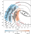 |
Fig. 3 Schematic picture of the Galactic arms as viewed from the north Galactic pole. Black spiral curves show the axes of the best-fit spiral magnetic arms of our model. The intensity of the color indicates the magnetic field strength in the Galactic plane ɀ = 0. The blue (orange) colored regions correspond to the magnetic field directed inward/clockwise (outward/counter-clockwise) as marked by the black arrows at the bottom of the plot. Black dot marks the Galactic center while an ellipse represents the Galactic bar. Red star marks the position of the Sun. Grey regions show the spiral arms as deduced from Gαiα observations. The pitch angle in the solar vicinity is 20°. |
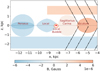 |
Fig. 4 Section of the best-fit GMF model in the plane y = 0, which is perpendicular to the Galactic plane and passes through the Sun (red star) and Galactic centre. Blue and orange regions are the magnetic arms, northern and southern toroidal field and the Local Bubble. The color map is the same as in Fig. 3. Black arrows show the direction of the X-shaped field. Red star marks the position of the Sun. |
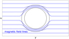 |
Fig. 5 Schematic drawing of the Local Bubble and surrounding magnetic field lines. The radius of the bubble in our model is fixed to 200 pc, while the best-fit thickness of its wall was found to be 30 pc. |
3.2 Thermal electrons
The calculation of the RMs requires the knowledge of the distribution of free electrons in the Galaxy. In our study we adopt the simple plane-parallel model of the density of free electrons ne:
 (9)
(9)
where n0 = 0.015 cm−3 is the mid-plane density and z0 = 1.57 kpc is the scale height. This corresponds to the best-fit model of Ocker et al. (2020) where it was shown to correctly predict the dispersion measures (DM) of pulsars located above the Galactic plane with |b| > 20°.
Similar values of n0 and z0 are used in more sophisticated models such as NE2001 (Cordes & Lazio 2002) and YMW16 (Yao et al. 2017). Additionally, these models take into account the increase of the density of electrons in the spiral arms whose effect is most pronounced near the Galactic plane |b| < 10°. Since in our analysis we treat the positions of magnetic arms as free parameters, the fixed positions of spiral arms of free electrons may significantly affect the results. For this reason we exclude the Galactic plane |b| < 10° from the analysis of RMs, as has already been stated in Sect. 2.2. At high Galactic latitudes the predictions of NE2001, YMW16 and plane-parallel models are approximately the same (Ocker et al. 2020) and thus the use of the latter model does not lead to a loss of accuracy. At intermediate latitudes 10° < |b| < 20° the enhancement of thermal electron number density in two nearby spiral gaseous arms may be important and can affect our results. This however should not change the results significantly since the errorbars for the RM bins in this latitude bands are large.
In addition, we take into account the modifications of the thermal electron density caused by the Local Bubble. On the wall of the Local Bubble the density is higher and depends on its thickness δrLB as
 (10)
(10)
This expression follows from the assumption that the explosions which formed the Local Bubble swept the ambient electrons of original constant density n0 to its walls. The value of the electron density inside the bubble is not important because there we assume the magnetic field to be zero.
3.3 Cosmic ray electrons
Cosmic ray electrons (CREs)4 are responsible for the Galactic synchrotron emission and are believed to be mostly accelerated by Galactic supernovae. Their propagation in the Galaxy (Moskalenko & Strong 1998; Orlando & Strong 2013) is of a diffusive nature and can be described by combined diffusion in the regular and turbulent magnetic fields.
In a simplified picture, CRE propagation can be describe as an isotropic diffusion determined by the single diffusion coefficient D0. We modeled the distribution of the CRE in the Galaxy using the numerical code DRAGON (Evoli et al. 2017), taking into account CRE energy losses by the inverse Compton scattering and the synchrotron emission. As a template for synchrotron losses we used the modified version of Jansson & Farrar (2012b) turbulent magnetic field with the normalisation of all arms set to 5 µG.
An isotropic diffusion is assumed to be within the simulation volume of radius RCRE = 16 kpc and the halo height of H = 4 kpc. We neglected anisotropic diffusion and assumed also that the diffusion coefficient is spatially independent. The dependence on the CRE rigidity R was taken to be the following:
 (11)
(11)
where D0 = 3.6 × 1028 cm2/s is the diffusion coefficient at rigidity R0 = 4 GV and δ = 0.47 is the spectral index. The propagation parameters H, D0 and δ were chosen based on the analysis of secondary-to-primary ratios by De la Torre Luque et al. (2024). Similar values were found in other studies, see Korsmeier & Cuoco (2021). The sources of cosmic rays were assumed to be distributed in the Galaxy according to Lorimer et al. (2006). The dynamic range of the simulation goes from 1 GeV up to 1 TeV. Our resulting CRE distribution is the sum of the distribution of primary electrons and secondary electrons and positrons produced in interactions of cosmic ray protons. We note that the contribution of secondary leptons to the total CRE density does not exceed 10% at energies of interest. Finally, we normalise the distribution to the local measurements by the Alpha Magnetic Spectrometer (AMS-02) experiment (Aguilar et al. 2019), as shown in Fig. C.1.
Modelling the Fan region requires an additional CRE component in the Perseus arm compared to the DRAGON output. Denoting as L the length of the arm axis starting from its origin we increase the CRE density in the Perseus arm according to the bump-like profile:
 (12)
(12)
where n0 is the CRE density on the solar vicinity, f = 0.7 is the relative amplitude of the additional bump, the parameter k = 2 kpc controls the sharpness of the bump boundaries, and L1 and L2 determine their coordinates. As a result, the CRE density is enhanced roughly in the direction from l ≃ 110° to l ≃ 180°. The parameters L1,2 were fixed from the geometry of the Fan region. The amplitude of the enhancement was also fixed; its value in the fit is largely degenerate with the amplitude of the magnetic field.
To the contrary, we do not consider the modification of the CRE density on the wall of the Local Bubble. Studying propagation of cosmic rays with full account of the details of the local magnetic field constitutes a separate problem and is beyond the scope of this paper.
Ideally, the CRE propagation should be fitted together with the GMF and include the effects of anisotropic diffusion. In practice, diffusion of CRE in space-dependent realistic GMF is a difficult problem which has not been solved so far Giacinti et al. (2014); Kachelriess & Semikoz (2019). In this sense the additional CRE component required for the Fan region in our model may indicate the necessity for deviation from the simplified isotropic picture.
Given the space and energy distributions of CRE in the Galaxy we calculate synchrotron Stokes Q and U parameters starting from the synchrotron emission of a single electron (Landau & Lifschits 1975). We thus do not adopt the commonly used power-law approximation of the electron spectrum for the volume emissivity and instead integrate numerically over the CRE spectrum. This allow us to take into account the curvature of the CRE spectrum as well as it’s variation over the line of sight.
4 Results of the global fit
The fitting of the model is performed by minimising the χ2. We first adjusted individual GMF components, as well as their various combinations until we reproduced qualitatively the key features of the data, and only then performed the combined fit. The multi-parametric optimisation was performed with the Nelder–Mead minimisation method. To test whether the found minimum is a global one, we repeated the minimisation with several different sets of initial parameters and varied the fitting step sizes. In all cases, the fit converged to the same parameter values, increasing the reliability of the results. After the convergence of the fit, we estimated the uncertainty of each parameter based on the curvature of the fit at the minimum (Press et al. 2007). Also, during the calculation of uncertainties, we ensured that the best- fit parameters correspond to the minimum of χ2 by computing the derivatives of χ2 with respect to each parameter and verifying that they are close to zero.
The model is fitted to the binned data as described in Sect. 2.1 with the binning scheme shown in Fig. 2. We used only those bins, which are left after removing outliers and masking. All the data bins and corresponding errorbars used for fitting are shown with black points in Figs. C.2, C.3, and C.45. For each data bin we evaluated the model up to the distance of 30 kpc from the position of the Sun in the direction of the line of sight (LOS) passing through the center of the bin. We checked that if we take ten evenly distributed LOSes per bin, the resulting χ2 changes very slightly, by 1–2%. Therefore, for the sake of saving computational time during fitting, we used only the central LOS.
The results of the global fit are presented in Fig. 6 which shows the comparison between the model (left column) and the masked data (right column) for three quantities: the RMs and the Q and U polarisation parameters. The polarised intensity map is shown in Fig. C.6. One may observe an overall qualitative agreement between the model and data maps. The best-fit total χ2/ndf is 1.36. The breakup of χ2 for the corresponding three contributions is given in Table 1, first three columns. The last two columns show what these quantities would be if the errors were calculated as mere variances in the bins, after removal of outliers. The over-estimation of errors in that case is obvious. The bin-by-bin comparison between the model and the data is given in Appendix C. The maps of residuals are shown in Fig. C.5.
The best-fit parameters of the model are summarised in Table 2. The strength of the magnetic field in the Local Arm was found to be 3.5 µG which is higher than previously thought. The increased strength of the field is a consequence of making the shape of the cross section of the Local Arm a free parameter (the squircle parameter n). In previous models a constant height of the disc across the arms was assumed. To the contrary, in our model the best-fit value is n = 1.45 causing the Local magnetic arm to be thicker in the center than above the Sun, see Fig. 4. This shape of the cross section significantly improves the fit allowing for stronger field in the direction of the outer Galaxy. As a result, the model better describes the wave-like pattern in the RM maps of the outer Galaxy between 1 ~ 90° and 1 ~ 270°, Fig. C.2.
In the neighboring Sagittarius-Carina arm in the direction of the Galactic center the magnetic field was found to be about 1.3 µG, which is weaker than the field in the Local Arm. In addition, its direction is opposite to that of the field in the Local Arm. Reversing the field direction in the Sagittarius-Carina arm (so that it aligns with the direction of the field in the Local Arm) while keeping the same strength worsens the RM χ2 by Δχ2 ≈ 110. Thus, we confirm the field reversal in accordance with Han & Qiao (1994) and Pshirkov et al. (2011).
Similarly, we confirm the necessity of the X-field. Setting it to zero increases the total chi-square by Δχ2 ≈ 260. The best- fit strength of the X-field near the Galactic plane was found to be 2 µG which is twice as large as in the base model of Unger & Farrar (2024). Our model prefers a sharp drop of the X-field strength at the Galactic radius of about 6 kpc. We discuss below in Sect. 5.2 how much it costs in terms of χ2 to extend the X-type field to the solar vicinity as suggested by the arguments based on the escape of Galactic cosmic rays.
The toroidal halo field is one of the key components of the model. If one sets the field in the toroidal halo to zero, the total chi-square nearly doubles: Δχ ≈ 1010. In the best-fit configuration the radial extensions of the norther and southern tori were found to be different, with the southern torus being larger than the northern one. However, the significance of this difference is not strong. When both tori are forced to have the same radius, the best-fit value of this common radius is rmax = 13.5 kpc, which worsens the fit by only Δχ2 ≈ 20.
Inclusion of the Local Bubble is a distinctive and novel feature of our model. As explained in Sect. 5.1, we approximated it as a spherical shell of finite thickness with a compressed magnetic field on its wall. Notably, the fitted parameters of the Local Bubble were found to be close to those known from other observations. The best-fit thickness of the Local Bubble wall in our model is δrLB = 30 pc which is in perfect agreement with the typical thickness of 35 pc determined in the recent analysis of O’Neill et al. (2024b) based on the distribution of the local dust. Given that the radius of the bubble was fixed to 200 pc the field strength in the most compressed regions of the wall reaches ~10–14 µG in accordance with Andersson & Potter (2006), Medan & Andersson (2019) and Kalberla & Haud (2023). To be more precise, using the Chandrasekhar-Fermi method Andersson & Potter (2006) found the plane-of-the-sky strength of the magnetic field  in the wall of the Local Bubble toward (l, b) ≈ (300°, 0°). This is in good agreement with the B⊥ = 11 µG predicted by our model in the same direction.
The best-fit direction of the bubble field before compression in our model is (lLB, bLB) = (230°, −2°), which is nearly opposite to the field of the Local Arm which has (l, b) = (70°, 0°). Remarkably, Pelgrims et al. (2020) found that the direction of the pre-compressed bubble field lies in the range (l, b) ≈ (72° ± 1°, 15° ± 2°) by analysing the polarised emission of the dust in the Galactic polar caps with |b| > 60°. Similar initial direction was found in a more recent analysis of the dust emission by O’Neill et al. (2024a). In view of the sign ambiguity inherent in the synchrotron polarisation data, this is in perfect agreement with our fit. In fact, in our fit the reversed (as compared to the Local Arm) direction is preferred only by the RM data. It is worth noting, however, that the Local Bubble contribution to the RM strongly depends on the shape of the bubble wall, and so the problem of the opposite field orientation should be re-examined together with a more accurate modelling of the bubble.
The best-fit position of the center of the Local Bubble was found to be shifted by ~100 pc from the position of the Solar System mostly in the direction of the positive y-axis. This is also generally consistent with the observations of the dust (Pelgrims et al. 2020; O’Neill et al. 2024b). Overall, the contribution from the Local Bubble is strongly favoured by the data. Its removal worsens the fit by Δχ2 ≈ 660.
The shape and overall brightness of the Fan region in our model generally matches the observations, as one can see from Fig. 6. The main contributions come from the Local Arm and the Perseus Arm. The parameters of the former are strongly constrained by the RM data. Adjusting mainly the parameters of the Perseus Arm allowed us to fit the Fan region. The correct vertical extension of the Fan region was achieved by fitting the (outer) vertical height of the Perseus Arm which converged to rz = 1.2 kpc. The field strength in the inner part around the Galactic plane was found to be 5.5 µG in order to reproduce the brightest part of the Fan region at |b| < 10°. In the outer part of the Perseus Arm the best-fit field strength is about 3.5 µG. Note, that the direction of the field (clockwise) in the Perseus arm was fixed to be the same as in the Local arm.
The common pitch angle of the spiral magnetic field arms was an independent parameter of the fit and converged to the value around ɑ0 = 20°. As one can see from Fig. 3 this is close to the pitch angle of spiral arm segments as inferred from the Gaia data (Poggio et al. 2021). Despite the Galactic plane being masked out in the RM data, the fit is still sensitive to the pitch angle. For the RM skymap the sensitivity is mostly driven by the two nearest spiral arms (Local arm and Sagittarius-Carina Arm) which give significant contribution to the RM signal even at |b| > 20°. Additionally, in the polarisation skymaps the signal from the Fan region depends strongly on the pitch angle of the Local and Perseus arms, see Sect. 5.4.
The result of the global fit.
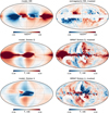 |
Fig. 6 RM (top row) and polarised synchrotron skymaps for Stokes Q (middle row) and Stokes U (bottom row) produced with the best-fit model (left column) in comparison with the data (right column). Masks on the data maps are discussed in the Sect. 2.2. |
Parameters of the model.
5 Discussion
5.1 Local Bubble and nearby loops
The Local Bubble introduced in our model significantly improves the fit for the polarisation data and, to a lesser extent, for the RMs. Below we discuss its role in these fits in more detail.
On the RM skymap the effect of the Local Bubble is clearly visible around the northern polar cap. In this region between 0° ≲ l ≲ 180° the Local Bubble gives a positive contribution to the RM which appears as a nearly uniform orange blur in Fig. 6. In the binned representation one can see this area as three data bands with 50° < b < 80° with mostly positive RMs, see Fig. C.26. This is the region of the RM sky that forces the field of the bubble to take direction opposite of the Local Arm. We should stress, however, that the sign and the amplitude of the bubble contribution to the RM depends significantly on the shape of its wall and the relative position of the solar system within the bubble. For instance, in our model where the bubble is spherical, this contribution can be set to zero by placing the solar system in the center as the field on the wall, which is purely tangential, is then perpendicular to the line of sight for all directions. It is therefore clear that a more detailed modelling of the bubble shape is required to firmly determine whether the direction of the field is parallel or antiparallel to the field in the Local Arm.
The sign flip of the initial bubble field has no effect on the polarisation maps. For both initial directions the Local Bubble produces the correct shape of the signal in Q and U maps near the Galactic poles, provided the bubble field is aligned to that in the Local Arm. The bubble contribution then almost completely compensates the deficit of the polarised intensity resulting from the other components when they are normalised to the RM data. It thus works similarly or even better than the striation of the magnetic fields assumed in previous works. We therefore believe that the alignment of the fields in the bubble and the Local Arm is a more robust result of our fit than the flipped direction of the bubble field which may be an artifact of our over-simplified modelling of the bubble geometry.
The role of the Local Bubble in fitting the polarisation data is illustrated in Fig. 7 which shows the polarised intensity PI =  integrated over the polar caps above given Galactic latitude b, as a function of b. The thick dashed line shows the fractional contribution of the “halo” part of the field defined here as everything at |z| > 1 kpc, normalised to the full model. The thick solid line shows the contribution of the “halo” and the Local Bubble, without other “disc” fields at |z| < 1 kpc. One can see that these two contributions together practically saturate the PI at high latitudes in roughly equal shares. For comparison, the same quantity is plotted in the model of Unger & Farrar (2024) with (thin solid curve) and without (thin dashed curve) the striation. The effects of the Local Bubble and striation are quite similar. The contribution of the Local Bubble to the Stokes U is explicitly shown in the Fig. 8.
The significance of the Local Bubble can also be understood with the simple analytical estimate. The brightness of the PI is proportional to the square of the magnetic field B2, the CR electron density nCRE(z) and the distance d. At high Galactic latitudes in the model of Unger & Farrar (2024) the main contribution to the PI comes from the toroidal halo, which starts at z ~ 1 kpc and has a width of d ~ 1 kpc. Thus PIhalo ∝ (3µG)2 nCRE(1 kpc) ⋅ kpc. At the same time the contribution from the Local Bubble reads: PILB ~ (10µG)2 nCRE(0) ⋅ 0.03 kpc. Noting that nCRE(1 kpc) ~ nCRE(0)/2 one comes to the conclusion that both contributions are approximately equal:
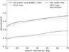 |
Fig. 7 Polarised intensity of the halo and halo+Local Bubble above a given latitude b normalised to the polarised intensity of the full model in the same region of the sky. In this plot ‘Halo’ refers to everything above |ɀ| > 1 kpc. See the main text for a discussion. |
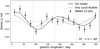 |
Fig. 8 Profile of the Stokes U signal calculated with the full model and the contribution from the Local Bubble. |
 (13)
(13)
The Local Bubble also affects propagation of cosmic rays from nearby sources. In particular, it helps to explain the cosmic ray flux at the knee by a contribution from the Vela supernova remnant (Bouyahiaoui et al. 2019). Also, interactions of cosmic rays with the gas on the walls of the Local bubble can give a significant contribution to the astrophysical neutrino flux (Andersen et al. 2018; Bouyahiaoui et al. 2020).
There are other large-scale anomalies in the data which are also, presumably, due to supernova bubbles, but viewed from outside, such as Loop I, Loop II, Loop III, etc. The fact that these anomalies are prominent on the polarisation sky suggests that the contribution of the Local Bubble is also sizeable. Inversely, it is possible that these anomalies can also be modelled in a similar way and included in the fit, rather than masked (Thomson et al. 2021). We leave this interesting question for future work.
5.2 Local X-shape field and escape of cosmic rays
The ratio of secondary to primary fluxes of cosmic rays indicates that locally most of the cosmic rays escape from the Galaxy before interaction with the interstellar gas (for the review see Kachelriess & Semikoz (2019) and references therein). In the simplified models of cosmic ray propagation the escape is described by diffusion. However, for pure turbulent field the required diffusion coefficient turns out to be too high, corresponding to unrealistically small magnetic field of the order of 10–5 µG. In Giacinti et al. (2018) it was shown that local z- component of the coherent GMF with the strength of a fraction of µG can resolve this cosmic ray escape problem. In the recent collection of GMF models of Unger & Farrar (2024) the local z- component is present in most of the models (see Fig. 16 in Unger & Farrar 2024).
In our best-fit model the X-field vanishes beyond the galacto- centric radius of 6.2 kpc. Adding the local z-component beyond 6.2 kpc with the strength of 0.2 µG slightly worsens the fit. If the direction of this additional component is the same as the direction of the X-field (i.e. towards positive z) the increase in the chi-square is Δχ2 ≈ 90. For the opposite direction the worsening is smaller, Δχ2 ≈ 30. In both cases all the increase comes from the RM fit since this field is too weak to contribute to the polarised intensity which is quadratic in the magnetic field strength. On the other hand, the contribution to the RM is of the same order as the effect of the Local Bubble discussed in Sect. 5.1. Thus, the search for such a weak additional component can only be performed together or after the accurate modelling of the Local Bubble.
5.3 Fan region
The Fan region is a bright feature of the radio sky located near the Galactic plane roughly in the direction 90° < l < 180°. It is visible as a red spot in the Stokes Q meaning that it contains magnetic field mostly parallel to the Galactic plane.
The distance to the Fan region remains uncertain. For a long time it was believed to be a local feature due to its exceptional brightness, high degree of polarisation and bubble-like shape. In particular, West et al. (2021) reproduced the brightness and the shape of the Fan region and Loop I with a bundle of local, narrow magnetic filaments with a width of ~20 pc possessing strong magnetic field of about 24 µG.
However, the model of West et al. (2021) seems to be in tension with recent observations at lower frequencies. First, there are indications that the Loop-I is not a local feature but a Galactic-scale outflow located at 3–5 kpc from the Galactic center (Zhang et al. 2024; Churazov et al. 2024). Second, Hill et al. (2017) argued that at least 30% of the polarised emission of the Fan region at frequencies around 1 GHz or higher must come from a distance of 2 kpc or more. The conclusion of Hill et al. (2017) was based on the observation that the portions of the 1.5 GHz Fan region emission are depolarised by ≈30% by distant ionised gas structures, indicating that a corresponding fraction of the emission originates from more than 2 kpc away. Additional evidence comes from the observations of the Radcliffe Wave located 0.5–1 kpc away in the direction to the Fan region (Alves et al. 2020). Based on the orientation of the magnetic field of the Radcliffe Wave Panopoulou et al. (2024) concluded that it is unlikely that the Fan region is at a distance <1 kpc.
In this regard, our model is the first attempt to demonstrate that the Fan region can be naturally incorporated as a part of the large-scale coherent GMF, as suggested by Hill et al. (2017). In contrast, in previous GMF models, the Fan region was considered a local feature and was either masked out or ignored.
The two main ingredients that allowed us to fit the Fan region are a larger (compared to previous models) pitch angle of the disc field and increased electron density in the Perseus arm. The former shifts the position of the peak intensity towards 1 ≈ 135°–140°, while the latter allows to reach the required brightness. The larger pitch angle was already predicted by Hill et al. (2017). Using simple geometrical analysis Hill et al. (2017) concluded that in order to fit the Fan region into the large-scale GMF model the pitch angle of the magnetic field in the disc should be in the range 15°–20°. The pitch angle of our model converged to 20° thus confirming the conclusions of Hill et al. (2017).
On the other hand, the increased CRE density in the Perseus arm may indicate either an efficient CRE transport along the arm due to the anisotropic diffusion or the presence of the local cosmic ray accelerators. This increase in our model was introduced artificially. More reliable distribution could be obtained by including the aforementioned effects into the CR propagation codes such as GALPROP Strong & Moskalenko (1998); Porter et al. (2022) or DRAGON Evoli et al. (2017). We note also that the exact distribution of the magnetic field along the LOS (in particular towards the Fan region) cannot be reliably inferred without invoking the tomographical methods.
5.4 Striated field and stability of the results
The model presented in this study is quite different from the existing ones in several respects, notably it has two additional components (the Local Bubble and the Fan region), the disc field pitch angle of 20° and zero striated fields. It is therefore instructive to check how these new features affect each other and the overall structure of the GMF model.
As a first test we included the striation coefficient ξ as an additional free parameter of the fit. Following the definition from Unger & Farrar (2024) the magnetic field strength used for the calculation of the synchrotron skymaps was rescaled as B′ = B(1 + ξ). Performing the fit with all the components of our model and this additional free parameter, the best-fit value of ξ was found to be compatible with zero: ξ = 0.01 ± 0.03. This is to be expected since the striation factor affects only the synchrotron intensity while the Local Bubble improves also the RM model, and thus the latter is preferred by the fit. On the other hand, the fit without the Local Bubble (with the magnetic field strength on the bubble wall set to zero) and without the additional CRE component in the Perseus arm resulted in ξ ≈ 0.3 compatible with ξ = 0.346 in the base model of Unger & Farrar (2024), but yielded a poorer fit for the RMs.
Second, we explored the reason of larger pitch angle in our model. We found that the fit of only RM data prefers the pitch of about 13°. However, the profile of the best fit χ2 as a function of the pitch angle is flat between 10° and 20°: the best fit χ2 worsens by only Δχ2 ≈ 20 if the pitch is fixed to 20° instead of 13°. The same small pitch angle is found if the synchrotron data is included, but the Galactic plane and the Fan region are masked out, in agreement with Unger & Farrar (2024). The strong preference for the pitch angle of 20° is found after the inclusion of the Fan region. Thus we conclude that the fit prefers larger pitch to fit the Fan region. This worsens the RM fit, but only slightly.
5.5 General remarks
Our Galaxy is believed to be a typical representative of the class of spiral galaxies. Therefore, it appears likely that the structure of its magnetic field should be similar to that of other spirals. Below we discuss how well our model fits into the bulk of knowledge about other galaxies.
Our fit requires the presence of the disc and halo fields in our Galaxy, which were also found in external spiral galaxies observed so far. We found that the pitch angle of the disc field is close to that of spiral gaseous arms. The rough similarity of the magnetic and stellar pitch angles were also observed in other spirals (Beck et al. 2019).
From the polarisation observations of other galaxies one finds that the strongest field of the disc often resides in interarm regions, while the regular field in the gaseous arms is somewhat suppressed. As it is clear from Fig. 4, if our Galaxy was observed from outside, its spacial distribution of the polarised intensity would be the opposite: the brightest parts would rather coincide with the gaseous arms. In order to see whether this is an unavoidable feature of our model we replace the constant field in the arms by hollow magnetic profiles such that the magnetic field in the inner 70% of the arm section is zero. Notably, this change of the profile does not spoil the RM fit while shifting the strongest polarised emission regions to the interarm space. The polarisation skymaps also remain practically unchanged at latitudes above ~30º where the polarised emission is mostly produced by the Local Bubble and the magnetic tori. However, one should adjust the strength of the field in the arms to have the correct emission near the Galactic plane. We do not see any fundamental contradictions that would prevent this modification of the model. We leave the detailed analysis of this possibility for future work.
Another feature that is observed in some other galaxies is field reversals. As one can see from Fig. 3, our model has one field reversal in the disc. The galaxies with one reversal in the disc have also been observed, see Beck et al. (2019).
6 Conclusions
In this paper, we present a new model of the regular magnetic field in the Galactic halo, which we then use to understand the field everywhere except in the thin disc. The model makes use of the most recent catalogue of the Faraday RMs and the synchrotron polarisation data by WMAP at 23 GHz. It builds on the previously existing models; but apart from using the most recent data, it has several novel features as compared to previous works.
For the first time, we took into account the contribution of the magnetic field in the wall of the Local Bubble. By constructing an explicit, albeit rough model of the Local Bubble as a sphere with the compressed magnetic field concentrated in the thick wall, we show that its contribution to the polarised intensity can explain the observations at high Galactic latitudes without contradicting the RM data. This is in contrast with previous works where the deficit of the model polarised intensity in these regions had to be compensated by assuming the striation of the field. The best-fit parameters of the bubble were found to be in good qualitative agreement with the existing independent measurements.
For the first time, we have fitted the Fan region – the large bright region in the outer galaxy that was masked out in the previous works that were using the polarisation data. Arguments have recently been presented supporting the idea that a large part of the polarised emission in this region comes from distances of 1–2 kpc and thus cannot be explained by a local anomaly. In order to fit the overall brightness and morphology of the polarised emission we had to assume that the magnetic field in the Perseus arm varies along the arm cross section, being stronger in the inner part close to the disc.
With these new features included, the best-fit value of the pitch angle of the magnetic arms is found to be close to ~20º, which is about two times that found in previous works, but is in good agreement with recent Gaia measurements of the pitch angle of stellar arms neighbouring the Solar System.
Finally, we have developed a systematic method of error estimation that provides a way to control the relative contributions of datasets of different nature (the RM and polarisation data in our case) to the global fit. This method takes into account the errors of individual measurements, the statistics of measurements in the bins, and the contribution of fluctuations at length scales exceeding the bin size. We find that the errors estimated with this method are typically smaller than those used in previous works, thus increasing the constraining power of the data.
Data availability
Appendix C, which contains Figures C.1, C.2, C.3, C.4, C.5, and C.6 illustrating the model’s performance, can be found at https://zenodo.org/records/14579789.
Acknowledgements
We would like to thank Ioana Codrina Maris for illuminating discussions and Denis Allard for useful comments on the manuscript. Our special thanks to Michael Unger, Maxim Pshirkov and Vincent Pelgrims for thorough reading of the manuscript and numerous constructive comments. The work of AK and PT is supported by the IISN project No. 4.4501.18.
Appendix A Removal of outliers
Each data bin that we consider (a rectangular region on the sphere limited by lines of constant l and b), we fit with a Gaussian. Namely, we assume that the measurements contained within the bin are samples from a Gaussian distribution with unknown parameters. By fitting data with a Gaussian we determine the mean µ and width σ of this distribution, taking into account errors of individual measurements.
To do this we construct a special likelihood function ℒ. Denoting as µi and σi the mean and error of each measurement in the bin it reads:
 (A.1)
(A.1)
where N is the total number of measurements within the bin. Physically each integral under the product means the probability of observing the value µi given the parameters of the distribution µ and σ and an observational error σi. This likelihood explicitly relies on the assumption of Gaussianity of the errors and in the limit σi → 0 reduces to a standard likelihood function.
Evaluating the integral we find
 (A.2)
(A.2)
The best fit values of σ and µ are obtained by minimising the log likelihood χ2 = –2 log ℒ. When applied to the real data we use an iterative procedure which also allow us to self-consistently remove outliers. After fitting the bin we remove those measurements whose values deviate from the mean µ by more than  and then repeat the fitting. The algorithm terminates when no outliers are detected. As a final step we determine 1σ confidence intervals µ ± σµ and σ ± σσ by exploring the contour of
  .
.
An example of the bin is shown in Fig A.1. The best fit values as well as its uncertainties are shown in the legend. The resulting Gaussian curve is narrower than the histogram since it shows how the distribution would look like assuming zero measurement errors. In total the bin initially contained 245 sources, 8 of which were detected as outliers (only 6 are visible in the plot). Since the algorithm takes into account errors of individual measurements, we note that a source with an RM of about −30 rad/m2 and a large error is included in the fit, while a source with a smaller RM of ∼ 25 rad/m2 and a much smaller error is marked as an outlier.
 |
Fig. A.1 Example of RM bin fitted with the gaussian. Points at the bottom of the figure indicate individual measurements within the bin together with their observational errors. Black points were discarded as outlier during the fit, blue points mark the LOFAR LoTSS data and orange points mark all other data. Blue boxes show the histogram of all sources except for outliers. Orange curve is the gaussian obtained as a result of the fit to all data (including LOFAR) and the pale green band is 68% confidence interval of its µ. The parameters of this gaussian are indicated on the plot. The blue curve is the best-fit gaussian if only LOFAR LoTSS data is used. |
Appendix B Derivation of the bin variance
Here we derive the variances of the bins associated with the coherent fluctuations in the ISM. First we derive the formula and then discuss how it is applied to the data.
Assume that the observable f depends on the discrete positions xi and denote fi = f (xi). The positions are evenly spaced so that xi – xi–1 = ∆x for any i. Assume also that f can be represented as a sum of the signal f0 and a random noise ϵ:
 (B.1)
(B.1)
Consider then the quantity  which is the value of f averaged over N nearby positions, or in other words averaged over the bin of the size L = N ∆x
 (B.2)
(B.2)
We are interested in its variance  :
:
 (B.3)
(B.3)
The angle brackets here denote averaging over different realisations of the noise ϵ while keeping the same signal f0. We further assume that the statistical properties of the noise do not depend on the position xi and that the noise has zero mean <ϵ> = 0. Substituting B.1 and B.2 into B.3 one gets
 (B.4)
(B.4)
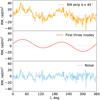 |
Fig. B.1 Fourier decomposition of the RM strip 40° < b < 50°. The upper panel shows the RM signal binned into 360 bins by l. The middle panel shows the first three Fourier modes (namely, the constant and 360° and 180° wavelength modes) of the RM signal, while the lower panel shows the contribution from all other modes except for the first three. |
As we assumed that the noise does not depend on x, the correlator <ϵjϵq> is the function only of the difference |xj – xq| but not the position itself. This allows one to evaluate the double sum in the Eq. B.4 by collecting and counting equal terms. Denoting the correlator <ϵjϵq> = r(|xj – xq|) one obtains the following expression:
 (B.5)
(B.5)
where r(x) is the correlation function of the noise. If the noise can be extracted from the measurements, this formula allows one to directly calculate the variance for the extended bin of the size L. In order to clarify the physical meaning of B.5 it is useful to consider the continuous limit ∆x → 0 in which the sum in B.5 can be replaced with an integral:
 (B.6)
(B.6)
Using Wiener-Khinchin theorem the correlation function r(x) can be expressed in terms of the noise power spectrum S(k)
 (B.7)
(B.7)
Substituting B.7 into B.6 and evaluating the integral over x one obtains
 (B.8)
(B.8)
When applied to the real data this equation transforms into a sum over the finite number of modes, where Sk can be calculated for example with the help of the Fast Fourier Transform (FFT). Thus, we arrive at Eq. B.9:
 (B.9)
(B.9)
In practice we calculate the power spectrum Sk by making a FFT of the data strips of constant latitude binned into 360 bins by longitude l. The FFT is made after removal of outliers, as described in Appendix A. An example of such transformation is shown in Fig. B.1 for the RM data strip. In order to exclude the contribution of the regular field we take into account only the modes with k ≥ kmin, where kmin = 3 corresponds to the wavelength of 90°.
References
- Aguilar, M., Ali Cavasonza, L., Alpat, B., et al. 2019, Phys. Rev. Lett., 122, 101101 [NASA ADS] [CrossRef] [Google Scholar]
- Alves, M. I. R., Boulanger, F., Ferrière, K., & Montier, L. 2018, A&A 611, L5 [NASA ADS] [CrossRef] [EDP Sciences] [Google Scholar]
- Alves, J., Zucker, C., Goodman, A. A., et al. 2020, Nature, 578, 237 [NASA ADS] [CrossRef] [Google Scholar]
- Andersen, K. J., Kachelrieß, M., & Semikoz, D. V. 2018, ApJ 861, L19 [NASA ADS] [CrossRef] [Google Scholar]
- Andersson, B. G., & Potter, S. B. 2006, ApJ 640, L51 [NASA ADS] [CrossRef] [Google Scholar]
- Anderson, C. S., Gaensler, B. M., Feain, I. J., & Franzen, T. M. O. 2015, ApJ 815, 49 [Google Scholar]
- Battye, R. A., Browne, I. W. A., Peel, M. W., Jackson, N. J., & Dickinson, C. 2011, MNRAS 413, 132 [NASA ADS] [CrossRef] [Google Scholar]
- Beck, R. 2001, Space Sci. Rev. 99, 243 [NASA ADS] [CrossRef] [Google Scholar]
- Beck, R. 2015, A&A Rev. 24, 4 [Google Scholar]
- Beck, R., Chamandy, L., Elson, E., & Blackman, E. G. 2019, Galaxies 8, 4 [NASA ADS] [CrossRef] [Google Scholar]
- Bennett, C. L., Larson, D., Weiland, J. L., et al. 2013, ApJS, 208, 20 [Google Scholar]
- Berkhuijsen, E. M., Urbanik, M., Beck, R., & Han, J. L. 2016, A&A 588, A114 [NASA ADS] [CrossRef] [EDP Sciences] [Google Scholar]
- Betti, S. K., Hill, A. S., Mao, S. A., et al. 2019, ApJ, 871, 215 [NASA ADS] [CrossRef] [Google Scholar]
- Bouyahiaoui, M., Kachelriess, M., & Semikoz, D. V. 2019, JCAP 01, 046 [Google Scholar]
- Bouyahiaoui, M., Kachelrieß, M., & Semikoz, D. V. 2020, Phys. Rev. D 101, 123023 [NASA ADS] [CrossRef] [Google Scholar]
- Brandenburg, A., & Ntormousi, E. 2023, ARA&A 61, 561 [CrossRef] [Google Scholar]
- Broten, N. W., MacLeod, J. M., & Vallee, J. P. 1988, Ap&SS 141, 303 [CrossRef] [Google Scholar]
- Brown, J. C., Taylor, A. R., & Jackel, B. J. 2003, ApJS 145, 213 [NASA ADS] [CrossRef] [Google Scholar]
- Brown, J. C., Haverkorn, M., Gaensler, B. M., et al. 2007, ApJ, 663, 258 [NASA ADS] [CrossRef] [Google Scholar]
- Burn, B. J. 1966, MNRAS 133, 67 [Google Scholar]
- Churazov, E., Khabibullin, I. I., Bykov, A. M., et al. 2024, A&A, 691, L22 [NASA ADS] [CrossRef] [EDP Sciences] [Google Scholar]
- Clarke, T. E., Kronberg, P. P., & Böhringer, H. 2001, ApJ 547, L111 [NASA ADS] [CrossRef] [Google Scholar]
- Clegg, A. W., Cordes, J. M., Simonetti, J. M., & Kulkarni, S. R. 1992, ApJ 386, 143 [CrossRef] [Google Scholar]
- Cordes, J. M., & Lazio, T. J. W. 2002, [arXiv:astro-ph/0207156] [Google Scholar]
- Costa, A. H., & Spangler, S. R. 2018, ApJ 865, 65 [NASA ADS] [CrossRef] [Google Scholar]
- Costa, A. H., Spangler, S. R., Sink, J. R., Brown, S., & Mao, S. A. 2016, ApJ 821, 92 [NASA ADS] [CrossRef] [Google Scholar]
- De la Torre Luque, P., Winkler, M. W., & Linden, T. 2024, JCAP, 05, 104 [Google Scholar]
- Evoli, C., Gaggero, D., Vittino, A., et al. 2017, JCAP, 02, 015 [Google Scholar]
- Farnes, J. S., Gaensler, B. M., & Carretti, E. 2014, ApJS 212, 15 [Google Scholar]
- Feain, I. J., Ekers, R. D., Murphy, T., et al. 2009, ApJ, 707, 114 [Google Scholar]
- Ferrière, K., & Terral, P. 2014, A&A 561, A100 [NASA ADS] [CrossRef] [EDP Sciences] [Google Scholar]
- Finkbeiner, D. P. 2003, Astrophys. J. Suppl. 146, 407 [NASA ADS] [CrossRef] [Google Scholar]
- Fletcher, A., Beck, R., Shukurov, A., Berkhuijsen, E. M., & Horellou, C. 2011, MNRAS 412, 2396 [CrossRef] [Google Scholar]
- Gaensler, B. M., Dickey, J. M., McClure-Griffiths, N. M., et al. 2001, ApJ, 549, 959 [Google Scholar]
- Giacinti, G., Kachelrieß, M., & Semikoz, D. V. 2014, Phys. Rev. D 90, 041302 [Google Scholar]
- Giacinti, G., Kachelriess, M., & Semikoz, D. V. 2018, JCAP 07, 051 [Google Scholar]
- Han, J. L., & Qiao, G. J. 1994, A&A 288, 759 [NASA ADS] [Google Scholar]
- Han, J. L., Manchester, R. N., Berkhuijsen, E. M., & Beck, R. 1997, A&A 322, 98 [NASA ADS] [Google Scholar]
- Han, J. L., Manchester, R. N., & Qiao, G. J. 1999, Mon. Not. Roy. Astron. Soc. 306, 371 [CrossRef] [Google Scholar]
- Han, J. L., Manchester, R. N., van Straten, W., & Demorest, P. 2018, ApJS 234, 11 [NASA ADS] [CrossRef] [Google Scholar]
- Heald, G., Braun, R., & Edmonds, R. 2009, A&A 503, 409 [NASA ADS] [CrossRef] [EDP Sciences] [Google Scholar]
- Hill, A. S., Landecker, T. L., Carretti, E., et al. 2017, MNRAS, 467, 4631 [NASA ADS] [CrossRef] [Google Scholar]
- Howard, A. M., & Kulsrud, R. M. 1997, Astrophys. J. 483, 648 [NASA ADS] [CrossRef] [Google Scholar]
- Hutschenreuter, S., Anderson, C. S., Betti, S., et al. 2022, A&A, 657, A43 [NASA ADS] [CrossRef] [EDP Sciences] [Google Scholar]
- Jansson, R., & Farrar, G. R. 2012a, Astrophys. J. 757, 14 [NASA ADS] [CrossRef] [Google Scholar]
- Jansson, R., & Farrar, G. R. 2012b, Astrophys. J. Lett. 761, L11 [CrossRef] [Google Scholar]
- Jansson, R., Farrar, G. R., Waelkens, A. H., & Enßlin, T. A. 2009, J. Cosmology Astropart. Phys. 2009, 021 [Google Scholar]
- Kachelriess, M., & Semikoz, D. V. 2019, Prog. Part. Nucl. Phys. 109, 103710 [NASA ADS] [CrossRef] [Google Scholar]
- Kaczmarek, J. F., Purcell, C. R., Gaensler, B. M., McClure-Griffiths, N. M., & Stevens, J. 2017, MNRAS 467, 1776 [NASA ADS] [Google Scholar]
- Kalberla, P. M. W., & Haud, U. 2023, A&A 673, A101 [NASA ADS] [CrossRef] [EDP Sciences] [Google Scholar]
- Kim, K. S., Lilly, S. J., Miniati, F., et al. 2016, ApJ, 829, 133 [NASA ADS] [CrossRef] [Google Scholar]
- Klein, U., Mack, K. H., Gregorini, L., & Vigotti, M. 2003, A&A 406, 579 [NASA ADS] [CrossRef] [EDP Sciences] [Google Scholar]
- Korsmeier, M., & Cuoco, A. 2021, Phys. Rev. D 103, 103016 [CrossRef] [Google Scholar]
- Lallement, R., Vergely, J. L., Babusiaux, C., & Cox, N. L. J. 2022, A&A 661, A147 [NASA ADS] [CrossRef] [EDP Sciences] [Google Scholar]
- Landau, L. D., & Lifschits, E. M. 1975, Course of Theoretical Physics, The Classical Theory of Fields (Oxford: Pergamon Press), 2 [Google Scholar]
- Law, C. J., Gaensler, B. M., Bower, G. C., et al. 2011, ApJ, 728, 57 [NASA ADS] [CrossRef] [Google Scholar]
- Livingston, J. D., McClure-Griffiths, N. M., Gaensler, B. M., Seta, A., & Alger, M. J. 2021, MNRAS 502, 3814 [NASA ADS] [CrossRef] [Google Scholar]
- Livingston, J. D., McClure-Griffiths, N. M., Mao, S. A., et al. 2022, MNRAS, 510, 260 [Google Scholar]
- Lorimer, D. R., Faulkner, A. J., Lyne, A. G., et al. 2006, MNRAS, 372, 777 [NASA ADS] [CrossRef] [Google Scholar]
- Ma, Y. K., Mao, S. A., Stil, J., et al. 2019, MNRAS, 487, 3432 [CrossRef] [Google Scholar]
- Ma, Y. K., Mao, S. A., Ordog, A., & Brown, J. C. 2020, MNRAS 497, 3097 [NASA ADS] [CrossRef] [Google Scholar]
- Mao, S. A., Gaensler, B. M., Stanimirovic, S., et al. 2008, ApJ, 688, 1029 [NASA ADS] [CrossRef] [Google Scholar]
- Mao, S. A., Gaensler, B. M., Haverkorn, M., et al. 2010, ApJ, 714, 1170 [NASA ADS] [CrossRef] [Google Scholar]
- Mao, S. A., McClure-Griffiths, N. M., Gaensler, B. M., et al. 2012a, ApJ, 755, 21 [NASA ADS] [CrossRef] [Google Scholar]
- Mao, S. A., McClure-Griffiths, N. M., Gaensler, B. M., et al. 2012b, ApJ, 759, 25 [NASA ADS] [CrossRef] [Google Scholar]
- Medan, I., & Andersson, B. G. 2019, ApJ 873, 87 [NASA ADS] [CrossRef] [Google Scholar]
- Minter, A. H., & Spangler, S. R. 1996, ApJ 458, 194 [NASA ADS] [CrossRef] [Google Scholar]
- Mora, S. C., & Krause, M. 2013, A&A 560, A42 [NASA ADS] [CrossRef] [EDP Sciences] [Google Scholar]
- Moskalenko, I. V., & Strong, A. W. 1998, Astrophys. J. 493, 694 [CrossRef] [Google Scholar]
- Moss, D., & Sokoloff, D. 2008, A&A 487, 197 [NASA ADS] [CrossRef] [EDP Sciences] [Google Scholar]
- Ocker, S. K., Cordes, J. M., & Chatterjee, S. 2020, Astrophys. J. 897, 124 [NASA ADS] [CrossRef] [Google Scholar]
- O’Neill, T. J., Goodman, A. A., Soler, J. D., Zucker, C., & Han, J. J. 2024a, ApJ, submitted [arXiv:2410.17341] [Google Scholar]
- O’Neill, T. J., Zucker, C., Goodman, A. A., & Edenhofer, G. 2024b, ApJ, 973, 136 [NASA ADS] [CrossRef] [Google Scholar]
- Oren, A. L., & Wolfe, A. M. 1995, ApJ 445, 624 [NASA ADS] [CrossRef] [Google Scholar]
- Orlando, E., & Strong, A. 2013, Mon. Not. Roy. Astron. Soc. 436, 2127 [CrossRef] [Google Scholar]
- O’Sullivan, S. P., Purcell, C. R., Anderson, C. S., et al. 2017, MNRAS, 469, 4034 [CrossRef] [Google Scholar]
- O’Sullivan, S. P., Shimwell, T. W., Hardcastle, M. J., et al. 2023, MNRAS, 519, 5723 [CrossRef] [Google Scholar]
- Panopoulou, G. V., Zucker, C., Clemens, D., et al. 2024, A&A, submitted [arXiv:2406.03765] [Google Scholar]
- Pelgrims, V., Ferrière, K., Boulanger, F., Lallement, R., & Montier, L. 2020, A&A 636, A17 [EDP Sciences] [Google Scholar]
- Planck Collaboration Int. XLII. 2016, A&A, 596, A103 [NASA ADS] [CrossRef] [EDP Sciences] [Google Scholar]
- Poggio, E., Drimmel, R., Cantat-Gaudin, T., et al. 2021, A&A, 651, A104 [NASA ADS] [CrossRef] [EDP Sciences] [Google Scholar]
- Porter, T. A., Johannesson, G., & Moskalenko, I. V. 2022, Astrophys. J. Supp. 262, 30 [NASA ADS] [CrossRef] [Google Scholar]
- Press, W. H., Teukolsky, S. A., Vetterling, W. T., & Flannery, B. P. 2007, Numerical Recipes 3rd Edition: The Art of Scientific Computing, 3rd edn. (USA: Cambridge University Press) [Google Scholar]
- Pshirkov, M. S., Tinyakov, P. G., Kronberg, P. P., & Newton-McGee, K. J. 2011, Astrophys. J. 738, 192 [CrossRef] [Google Scholar]
- Pshirkov, M. S., Tinyakov, P. G., & Urban, F. R. 2013, Mon. Not. Roy. Astron. Soc. 436, 2326 [CrossRef] [Google Scholar]
- Ranchod, S., Mao, S. A., Deane, R., et al. 2024, A&A, 686, A104 [NASA ADS] [CrossRef] [EDP Sciences] [Google Scholar]
- Riseley, C. J., Lenc, E., Van Eck, C. L., et al. 2018, PASA, 35, 43 [Google Scholar]
- Riseley, C. J., Galvin, T. J., Sobey, C., et al. 2020, PASA, 37, e029 [Google Scholar]
- Rossetti, A., Dallacasa, D., Fanti, C., Fanti, R., & Mack, K. H. 2008, A&A 487, 865 [NASA ADS] [CrossRef] [EDP Sciences] [Google Scholar]
- Roy, S., Rao, A. P., & Subrahmanyan, R. 2005, MNRAS 360, 1305 [NASA ADS] [CrossRef] [Google Scholar]
- Schnitzeler, D. H. F. M. 2010, Mon. Not. Roy. Astron. Soc. 409, L97 [Google Scholar]
- Schnitzeler, D. H. F. M., Carretti, E., Wieringa, M. H., et al. 2019, MNRAS, 485, 1293 [NASA ADS] [CrossRef] [Google Scholar]
- Shanahan, R., Lemmer, S. J., Stil, J. M., et al. 2019, ApJ, 887, L7 [NASA ADS] [CrossRef] [Google Scholar]
- Shaw, V., van Vliet, A., & Taylor, A. M. 2022, Mon. Not. Roy. Astron. Soc. 517, 2534 [CrossRef] [Google Scholar]
- Simard-Normandin, M., Kronberg, P. P., & Button, S. 1981, ApJS 45, 97 [NASA ADS] [CrossRef] [Google Scholar]
- Skalidis, R., & Pelgrims, V. 2019, A&A 631, L11 [NASA ADS] [CrossRef] [EDP Sciences] [Google Scholar]
- Soida, M., Krause, M., Dettmar, R. J., & Urbanik, M. 2011, A&A 531, A127 [NASA ADS] [CrossRef] [EDP Sciences] [Google Scholar]
- Strong, A. W., & Moskalenko, I. V. 1998, Astrophys. J. 509, 212 [CrossRef] [Google Scholar]
- Sun, X.-H., & Reich, W. 2010, Res. Astron. Astrophys. 10, 1287 [Google Scholar]
- Tabara, H., & Inoue, M. 1980, A&AS 39, 379 [Google Scholar]
- Taylor, A. R., Stil, J. M., & Sunstrum, C. 2009, ApJ 702, 1230 [Google Scholar]
- Taylor, A. R., Sekhar, S., Heino, L., et al. 2024, MNRAS, 528, 2511 [NASA ADS] [CrossRef] [Google Scholar]
- Terral, P., & Ferrière, K. 2017, A&A 600, A29 [NASA ADS] [CrossRef] [EDP Sciences] [Google Scholar]
- Thomson, A. J. M., Landecker, T. L., Dickey, J. M., et al. 2019, MNRAS, 487, 4751 [NASA ADS] [CrossRef] [Google Scholar]
- Thomson, A. J. M., Landecker, T. L., McClure-Griffiths, N. M., et al. 2021, MNRAS, 507, 3495 [NASA ADS] [CrossRef] [Google Scholar]
- Tinyakov, P. G., & Tkachev, I. I. 2002, Astropart. Phys. 18, 165 [NASA ADS] [CrossRef] [Google Scholar]
- Unger, M., & Farrar, G. R. 2024, ApJ 970, 95 [NASA ADS] [CrossRef] [Google Scholar]
- Vanderwoude, S., West, J. L., Gaensler, B. M., et al. 2024, AJ, 167, 226 [CrossRef] [Google Scholar]
- Van Eck, C. L., Brown, J. C., Stil, J. M., et al. 2011, ApJ, 728, 97 [Google Scholar]
- Van Eck, C. L., Haverkorn, M., Alves, M. I. R., et al. 2018, A&A, 613, A58 [NASA ADS] [CrossRef] [EDP Sciences] [Google Scholar]
- Van Eck, C. L., Brown, J. C., Ordog, A., et al. 2021, ApJS, 253, 48 [NASA ADS] [CrossRef] [Google Scholar]
- Van Eck, C. L., Gaensler, B. M., Hutschenreuter, S., et al. 2023, ApJS, 267, 28 [NASA ADS] [CrossRef] [Google Scholar]
- Vernstrom, T., Gaensler, B. M., Vacca, V., et al. 2018, MNRAS, 475, 1736 [NASA ADS] [CrossRef] [Google Scholar]
- Vidal, M., Dickinson, C., Davies, R. D., & Leahy, J. P. 2015, MNRAS 452, 656 [NASA ADS] [CrossRef] [Google Scholar]
- Watts, D. J., Basyrov, A., Eskilt, J. R., et al. 2023, A&A, 679, A143 [NASA ADS] [CrossRef] [EDP Sciences] [Google Scholar]
- West, J. L., Landecker, T. L., Gaensler, B. M., Jaffe, T., & Hill, A. S. 2021, ApJ 923, 58 [NASA ADS] [CrossRef] [Google Scholar]
- Wielebinski, R., & Krause, F. 1993, A&ARv 4, 449 [NASA ADS] [CrossRef] [Google Scholar]
- Wolleben, M., Fletcher, A., Landecker, T. L., et al. 2010, ApJ, 724, L48 [NASA ADS] [CrossRef] [Google Scholar]
- Wolleben, M., Landecker, T. L., Carretti, E., et al. 2019, AJ, 158, 44 [NASA ADS] [CrossRef] [Google Scholar]
- Wolleben, M., Landecker, T. L., Douglas, K. A., et al. 2021, AJ, 162, 35 [NASA ADS] [CrossRef] [Google Scholar]
- Xu, J., & Han, J. L. 2019, MNRAS 486, 4275 [NASA ADS] [CrossRef] [Google Scholar]
- Xu, J., & Han, J. L. 2024, ApJ 966, 240 [NASA ADS] [CrossRef] [Google Scholar]
- Yao, J. M., Manchester, R. N., & Wang, N. 2017, ApJ 835, 29 [NASA ADS] [CrossRef] [Google Scholar]
- Zhang, H.-S., Ponti, G., Carretti, E., et al. 2024, Nat. Astron., 8, 1416 [CrossRef] [Google Scholar]
The Appendix C is available at https://zenodo.org/records/14579789
The catalogue can be found online at the link https://github.com/CIRADA-Tools/RMTable
We note that the RM skymap of Hutschenreuter et al. (2022) while cleaned of outliers is not suitable for our purposes since the correlations between individual pixels of the map do not allow for the estimation of the errorbars of larger bins, see Sect. 2.1.
Throughout the paper by CRE we mean both relativistic electrons and positrons.
The Appendix C is available at https://zenodo.org/records/14579789
The Appendix C is available at https://zenodo.org/records/14579789
All Tables
All Figures
|
Fig. 1 Compilation of the data used in this paper. Upper panel: extra-galactic RM skymap, smoothed and cleaned by Hutschenreuter et al. (2022). We note that in our main analysis, we start with the individual RMs from the CIRADA catalog. The RM skymap from Hutschenreuter et al. (2022) is shown for clearer visual representation. Middle and bottom panels: WMAP synchrotron Stokes Q and U skymaps at 23 GHz (Bennett et al. 2013). |
| In the text | |
|
Fig. 2 Binning scheme used in this analysis. The bins are rectangular in Galactic coordinates and are arranged in iso-latitude bands of 10° in width. The two equatorial bands are divided into 36 square 10° × 10° bins each. The number of bins in other bands is chosen in such a way as to get the closest approximation to equal-area bins. |
| In the text | |
|
Fig. 3 Schematic picture of the Galactic arms as viewed from the north Galactic pole. Black spiral curves show the axes of the best-fit spiral magnetic arms of our model. The intensity of the color indicates the magnetic field strength in the Galactic plane ɀ = 0. The blue (orange) colored regions correspond to the magnetic field directed inward/clockwise (outward/counter-clockwise) as marked by the black arrows at the bottom of the plot. Black dot marks the Galactic center while an ellipse represents the Galactic bar. Red star marks the position of the Sun. Grey regions show the spiral arms as deduced from Gαiα observations. The pitch angle in the solar vicinity is 20°. |
| In the text | |
|
Fig. 4 Section of the best-fit GMF model in the plane y = 0, which is perpendicular to the Galactic plane and passes through the Sun (red star) and Galactic centre. Blue and orange regions are the magnetic arms, northern and southern toroidal field and the Local Bubble. The color map is the same as in Fig. 3. Black arrows show the direction of the X-shaped field. Red star marks the position of the Sun. |
| In the text | |
|
Fig. 5 Schematic drawing of the Local Bubble and surrounding magnetic field lines. The radius of the bubble in our model is fixed to 200 pc, while the best-fit thickness of its wall was found to be 30 pc. |
| In the text | |
|
Fig. 6 RM (top row) and polarised synchrotron skymaps for Stokes Q (middle row) and Stokes U (bottom row) produced with the best-fit model (left column) in comparison with the data (right column). Masks on the data maps are discussed in the Sect. 2.2. |
| In the text | |
|
Fig. 7 Polarised intensity of the halo and halo+Local Bubble above a given latitude b normalised to the polarised intensity of the full model in the same region of the sky. In this plot ‘Halo’ refers to everything above |ɀ| > 1 kpc. See the main text for a discussion. |
| In the text | |
|
Fig. 8 Profile of the Stokes U signal calculated with the full model and the contribution from the Local Bubble. |
| In the text | |
|
Fig. A.1 Example of RM bin fitted with the gaussian. Points at the bottom of the figure indicate individual measurements within the bin together with their observational errors. Black points were discarded as outlier during the fit, blue points mark the LOFAR LoTSS data and orange points mark all other data. Blue boxes show the histogram of all sources except for outliers. Orange curve is the gaussian obtained as a result of the fit to all data (including LOFAR) and the pale green band is 68% confidence interval of its µ. The parameters of this gaussian are indicated on the plot. The blue curve is the best-fit gaussian if only LOFAR LoTSS data is used. |
| In the text | |
|
Fig. B.1 Fourier decomposition of the RM strip 40° < b < 50°. The upper panel shows the RM signal binned into 360 bins by l. The middle panel shows the first three Fourier modes (namely, the constant and 360° and 180° wavelength modes) of the RM signal, while the lower panel shows the contribution from all other modes except for the first three. |
| In the text | |
Current usage metrics show cumulative count of Article Views (full-text article views including HTML views, PDF and ePub downloads, according to the available data) and Abstracts Views on Vision4Press platform.
Data correspond to usage on the plateform after 2015. The current usage metrics is available 48-96 hours after online publication and is updated daily on week days.
Initial download of the metrics may take a while.