| Issue |
A&A
Volume 693, January 2025
|
|
|---|---|---|
| Article Number | A114 | |
| Number of page(s) | 15 | |
| Section | Stellar structure and evolution | |
| DOI | https://doi.org/10.1051/0004-6361/202451371 | |
| Published online | 07 January 2025 | |
Supernova shocks cannot explain the inflated state of hypervelocity runaways from white dwarf binaries
1
Institut für Physik und Astronomie, Universität Potsdam, Haus 28, Karl-Liebknecht-Str. 24/25, 14476 Potsdam-Golm, Germany
2
Dr Karl Remeis-Observatory & ECAP, Friedrich-Alexander University Erlangen-Nürnberg, Sternwartstr. 7, 96049 Bamberg, Germany
3
Max Planck Institut für Astrophysik, Karl-Schwarzschild-Straße 1, 85748 Garching bei München, Germany
4
Center for Astrophysics | Harvard & Smithsonian, 60 Garden Street, Cambridge, MA 02138, USA
5
Department of Astronomy and Theoretical Astrophysics Center, University of California, Berkeley, CA 94720-3411, USA
6
Institute of Science and Technology Austria (IST Austria), Am Campus 1, Klosterneuburg, Austria
7
Division of Physics, Mathematics and Astronomy, California Institute of Technology, 1200 E. California Blvd., Pasadena, CA 91125, USA
8
Department of Physics and Astronomy, Michigan State University, East Lansing, MI 48824, USA
9
Department of Computational Mathematics, Science, and Engineering, Michigan State University, East Lansing MI 48824, USA
⋆ Corresponding author; This email address is being protected from spambots. You need JavaScript enabled to view it.
Received:
3
July
2024
Accepted:
4
November
2024
Abstract
Recent observations have found a growing number of hypervelocity stars with speeds of ≈1500 − 2500 km s−1 that could have only been produced through thermonuclear supernovae in white dwarf binaries. Most of the observed hypervelocity runaways in this class display a surprising inflated structure: their current radii are roughly an order of magnitude greater than they would have been as white dwarfs filling their Roche lobe. While many simulations exist studying the dynamical phase leading to supernova detonation in these systems, no detailed calculations of the long-term structure of the runaways have yet been performed. We used an existing AREPO hydrodynamical simulation of a supernova in a white dwarf binary as a starting point for the evolution of these stars with the one-dimensional stellar evolution code MESA. We show that the supernova shock is not energetic enough to inflate the white dwarf over timescales longer than a few thousand years, significantly shorter than the 105 − 6 year lifetimes inferred for observed hypervelocity runaways. Although they experience a shock from a supernova less than ≈0.02 R⊙ away, our models do not experience significant interior heating, and all contract back to radii of around 0.01 R⊙ within about 104 years. Explaining the observed inflated states requires either an additional source of significant heating or some other physics that is not yet accounted for in the subsequent evolution.
Key words: supernovae: general / white dwarfs
© The Authors 2025
 Open Access article, published by EDP Sciences, under the terms of the Creative Commons Attribution License (https://creativecommons.org/licenses/by/4.0), which permits unrestricted use, distribution, and reproduction in any medium, provided the original work is properly cited.
This article is published in open access under the Subscribe to Open model. This email address is being protected from spambots. You need JavaScript enabled to view it. to support open access publication.
1. Introduction
Thermonuclear supernovae in white dwarf binaries can produce a hypervelocity runaway companion, and we are now discovering some of the fastest stars in our Galaxy that appear to have originated from this scenario (Shen et al. 2018a; El-Badry et al. 2023). While the growing number of observed candidates from such a scenario seems to confirm the importance of double white dwarfs as thermonuclear supernova progenitors, the stellar structure of these runaways is still poorly understood. This leaves an incomplete picture of the connection between these runaways in our Galaxy and the population of Type Ia supernovae observed in our Universe. In the dynamically driven double degenerate double detonation (D6) scenario, a white dwarf transfers mass to a more massive white dwarf through dynamically unstable Roche-lobe overflow (Guillochon et al. 2010; Dan et al. 2011, 2012; Pakmor et al. 2013; Shen et al. 2018b). This unstable mass transfer, mainly comprised of heavily compressed 4He, leads to a thermonuclear runaway through dynamical instabilities in the interaction between the accretion stream and the shell of the accretor. This can trigger a detonation. The shell detonation leads to a shock that traverses inside the white dwarf and converges in the carbon-oxygen core. At this stage, it is possible to ignite carbon and detonate the white dwarf (Fink et al. 2007; Kromer et al. 2010; Pakmor et al. 2013, 2022; Moll & Woosley 2013; Boos et al. 2021). Once this happens the accreting white dwarf effectively disappears and the donor star is ejected at its pre-supernova orbital speed and becomes a runaway star. Due to the compact nature of the stars, the secondary is very close to the primary before filling its Roche lobe. Therefore, the runaways can reach velocities of the order of 1000 − 2500 km s−1. For runaways observed with velocities above ≈1500 km s−1 that do not come from the Galactic centre (which could indicate a Hills 1988 mechanism origin), the D6 supernova scenario is the only way to explain their extreme velocities without relying on objects like intermediate-mass black holes.
All the observed D6 runaway candidates are peculiar. They have galactocentric velocities greater than 1000 km s−1; the fastest ones have velocities of ≈2500 km s−1. As they are unbound to the Galaxy and still observable, they cannot be more than 10 − 100 Myr removed from the supernova event. Moreover, their observed flight times to the Galactic disk – and in at least one case to SN remnants – suggest lifetimes of at most a few megayears. Due to the mass-radius relation of white dwarfs, these velocities directly imply that the donor white dwarfs must have been massive (> 1 M⊙) for the fastest runaways and (> 0.5 M⊙) for the slightly slower ones (Bauer et al. 2021). While the difference in composition of sub-Chandrasekhar mass white dwarfs can affect the mass-radius relation by a few per cent and lead to slightly different orbital velocities, these differences will be smaller than the uncertainties in observed orbital velocities due to uncertain distances. We also note the caveat that the preceding mass estimates assume a Roche-filling donor at the time of explosion. It may also be possible that the accretor detonates later when the donor is significantly beyond its Roche limit, so that the plunging donor star might reach higher velocities than when it fills its Roche lobe. In this case the mass of the runaway could be lower, down to 0.4 M⊙ (Dan et al. 2012). In any case, almost all of the observed white dwarfs are puffed up, most with radii of the order of 0.1 R⊙ instead of < 0.01 R⊙ as expected from their velocities. One possible explanation that has been suggested for this behaviour is post-shock induced heating due to the supernova, and by supernova ejecta material deposited on the surface. To date, some stellar evolution models have addressed the impact of supernova shocks on ejected subdwarfs in single-degenerate supernovae (Bauer et al. 2019), double-degenerate supernovae with a helium white dwarf donor (Wong et al. 2024), and Type Iax remnant stars (Zhang et al. 2019) to explain the observations of the runaways (Hirsch et al. 2005; Geier et al. 2015; Vennes et al. 2017; Raddi et al. 2018, 2019).
While these efforts have provided insights into the evolution of subdwarfs and partially burned white dwarfs, a detailed investigation into the evolution of the faster D6 runaways is still missing. As we show in this work, and as estimated analytically in Bauer et al. (2019), it is much more difficult for the supernova shock to strongly perturb the thermal state of a D6 WD donor than in the previously studied cases of subdwarf donors or Iax remnants. For this paper we improved upon previous work by carrying out the first full-scale stellar evolution calculation of such surviving white dwarfs. We utilised the result of an existing AREPO three-dimensional hydrodynamical simulation of binary white dwarfs that undergo a supernova explosion and end with a hypervelocity runaway donor remnant (Springel 2010; Pakmor et al. 2016, 2022; Weinberger et al. 2020). This simulation, taken from Pakmor et al. (2022), followed the evolution until shortly after double detonation of the primary white dwarf. In total, the runaway was evolved for 150 s after explosion when the ejecta are in homologous expansion and the surviving secondary white dwarf has settled into hydro-static equilibrium. We used this surviving donor as input into the one-dimensional open-source stellar evolution software Modules for Experiments in Stellar Astrophysics (MESA, Paxton et al. 2011, 2013, 2015, 2018, 2019; Jermyn et al. 2023).
The AREPO simulation provides profiles of the composition and thermal state of pre- and post-supernova configurations for the donor, which becomes a hypervelocity runaway. We used the entropy profiles to calculate the heating associated with the supernova shock. We used the result to create an approximate model of the heating for different masses of white dwarfs (0.5 to 1.1 M⊙) to explore how the subsequent evolution may depend on runaway mass. We then modelled the subsequent stellar evolution through the following 100 Myr, after which time these stars would be in the outer halo of the Galaxy and not observable. The mapping of only one available AREPO simulation is not exact when extrapolated to white dwarf binaries of other masses. The heating of a donor white dwarf likely has some dependence on mass since a more massive white dwarf will be closer to the supernova, but at the same time is more difficult to perturb due to its higher pressure and internal energy profile. As a first exploration based on the one available AREPO model, our work scales the heating from the 0.7 M⊙ simulation to higher masses, representing a maximally aggressive heating to place an upper limit on how long the white dwarfs can stay puffed up. In Section 2 we discuss the AREPO simulations and develop an approximate approach to generalise the heating we see in the one AREPO model to white dwarf donors of different masses. In Section 3 we present the evolution of all our models. Finally, in Section 4 we compare these models to recent observation of D6 runaways. We summarise our results in Section 5.
2. Simulations and relaxation
Our goal in this work is to model the long-term stellar evolution of the runaway donor in order to compare it with observed hypervelocity runaways. These runaways travel at speeds of the order of 1 − 2 kpc/Myr, so we expect that they would leave the Galaxy and become unobservable within about 10 Myr. We therefore want to compare evolutionary tracks with ages reaching a few megayear after explosion for typical observable runaways, though some could be younger. After the initial interaction with the SN ejecta and dynamical evolution over timescales of a few hundred seconds modelled in AREPO, the donor star should quickly settle (Shen et al. 2012; Schwab et al. 2012) into an approximately spherical and hydrostatic structure appropriate for modelling with a 1D stellar evolution code such as MESA for longer timescales. We neglect rotation in this work because even a tidally locked donor star will be significantly below critical rotation, and the energy in rotational shear in the AREPO model is negligible compared to other energy scales. In this section, we describe the initial dynamical evolution modelled in AREPO up to a point suitable to handing off to MESA for longer term evolution, along with the procedure for mapping from the 3D Arepo model into the eventual 1D hydrostatic structure for MESA.
2.1. Three-dimensional hydrodynamical explosion model
We start from an existing explosion simulation in AREPO of a double white dwarf system (Pakmor et al. 2022). This simulation starts with the late stages of inspiral of a binary system of two carbon-oxygen white dwarfs with masses of 1.05 M⊙ and 0.7 M⊙, respectively. The donor model starts with a 50/50 C/O core composition and a pure He envelope in the outer 0.03 M⊙. This helium mass is significantly higher than the mass required to support a double detonation (Shen et al. 2024), and almost an order of magnitude more than the helium shell masses of realistic WD models (e.g. Lawlor & MacDonald 2006). This is motivated by the need to have enough He mass transfer such that the accretor is sure to double-detonate. Accretion of helium-rich material from the less massive donor to the more massive accretor dynamically ignites a helium detonation in the helium shell of the accretor. The helium detonation propagates around the accretor and via compression ignites a detonation in the carbon-oxygen core of the accretor, similar to the classic double detonation scenario for Type Ia supernovae.
The accretor explodes as a Type Ia supernova. It disappears on a timescale of a few seconds, and hits the donor white dwarf with a strong shockwave on the way, that travels with a velocity of ∼10 000 km s−1. During this process, the donor white dwarf also burns its helium shell and loses its outer layers. If it survives the impact and does not also explode itself (Tanikawa et al. 2019; Pakmor et al. 2022; Boos et al. 2024; Shen et al. 2024), new material (in particular 56Ni) is deposited from the low-velocity tail of the supernova ejecta, resulting in a final mass of the donor of 0.67 M⊙. While the donor experiences a shock from the interaction with supernova ejecta, this shock is only strong enough to deposit significant entropy near the surface. The AREPO model also experiences some additional viscous heating during post-shock ringdown, but again, this is negligible in the core.
Due to its almost Lagrangian nature, AREPO can follow both the expanding supernova ejecta and the resolved surviving donor white dwarf for more than 100 s after the explosion. Here we use the surviving donor of this existing simulation as a starting point to study its subsequent evolution. We employ the composition and entropy profiles of the donor at the end of the AREPO simulation and insert them into MESA. Our donor is on the less massive end of the masses predicted from Roche-lobe filling donors based on observed runaway velocities. In this work we will also use the heating profile from this model to estimate the potential impact of supernova interaction for more massive WD donors as well. At this stage, creating a new simulation with more massive white dwarfs was not within the scope of this work. In reality, we expect that more massive WDs would be even harder to perturb with supernova shocks due to higher internal pressures (Bauer et al. 2019), and therefore our work represents an upper limit on supernova shock heating for the more massive models.
The final AREPO profile of the remnant contains composition information and spherically averaged 1D temperature-density pairs for different shells of the star. This profile differs from the initial profile of the donor due to the presence of heavy elements generated during the supernova explosion. The final composition profiles of the main elements with mass fractions max(Xn) > 10−4 within the donor and the remnant are shown as a comparison in Figure 1.
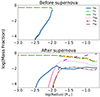 |
Fig. 1. Main elements and their composition profiles as a function of radius for the donor right before the supernova [top] and the runaway 150 s after the supernova [bottom] for mass coordinates, which remain bound after supernova explosion (< 0.661 M⊙). In particular, 56Ni dominates the mass fraction at the surface of the runaway. The surface helium content of the donor is less than 0.03 M⊙ as most of it has been accreted by the primary. |
Notably, there is a tail of helium from the envelope that is mixed deeply into the core of the surviving white dwarf. Figure 2 shows slices through the midplane of the donor white dwarf at the beginning of the binary simulation and just before the accreting white dwarf explodes in a supernova. The mixing of helium into its core is driven by shear on the surface. However, the refinement and derefinement in the AREPO moving mesh in this simulation during inspiral approaching mass transfer significantly enhances this shear mixing in an nonphysical manner. We checked this by changing the refinement of the donor surface separately (without re-running the entire simulation) and found the mixing to be negligible. Experimenting with the addition of resolution, we found the mixing to essentially completely disappear. While we can’t entirely exclude the possibility that some shear mixing could occur over much longer timescales than the dynamical AREPO simulation, these experiments confirm that the mixing seen in Figure 2 is a numerical artefact. Since we believe in particular the deep mixing is mostly artificial, we will evolve models of the surviving white dwarf where we remove this helium tail from the core by replacing any 4He with 12C in the inner 99% of the star by mass coordinate. The evolution of the original AREPO composition is provided in Appendix B.
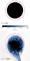 |
Fig. 2. Mass fraction of helium in the donor at two different times. Top panel: Helium mass fraction at the beginning of the simulation showing no mixing. Bottom panel: Mixing of helium in the donor just before the explosion of the accretor. The red line shows a contour of ρ = 104 g cm−3. During the accretion and inspiral the helium from the surface seeps into the deeper layers of the donor. |
2.2. Mapping the hydrodynamical result into 1D stellar evolution
To model the long-term evolution of the remnant runaway, we evolve it further in MESA (Paxton et al. 2011, 2013, 2015, 2018, 2019; Jermyn et al. 2023), an open-source one-dimensional stellar evolution code. The components of the MESA EOS blend relevant for this work are FreeEOS (Irwin 2004) near the surface of models, and HELM (Timmes & Swesty 2000) and Skye (Jermyn et al. 2021) for white dwarf cores. MESA uses tabulated radiative opacities primarily from OPAL (Iglesias & Rogers 1993, 1996), with low-temperature data from Ferguson et al. (2005) and the high-temperature, Compton-scattering dominated regime by Poutanen (2017). The electron conduction opacities are from Cassisi et al. (2007). Nuclear reactions are from JINA REACLIB (Cyburt et al. 2010), NACRE (Angulo et al. 1999) and additional tabulated weak reaction rates (Fuller et al. 1985; Oda et al. 1994; Langanke & Martínez-Pinedo 2000). Screening of reaction rates is included via the prescription of Chugunov et al. (2007), while thermal neutrino loss rates are from Itoh et al. (1996).
In order to map the change in thermal state of the white dwarf donor into MESA, we map the change in entropy that the donor star experiences as a result of interaction with the supernova ejecta. This is important, because when a supernova occurs in a close binary system, the ejecta interact with the donor in several ways. They cause a shock to propagate through the donor and directly deposit thermal energy in the interior. The ejecta also strip away material from the surface of the star. Moreover, they shock the helium shell of the donor white dwarf, which detonates and burns (Pakmor et al. 2022). Here we assume that the core of the donor does not explode as well (Pakmor et al. 2022; Shen et al. 2024). Essentially all of the ashes of the helium burning on the surface of the donor will be ejected. Interior fluid elements experience shock heating that can increase their entropy, followed by adiabatic decompression to a lower density configuration as the donor white dwarf settles into a less compact configuration at lower mass. Therefore, the specific internal energy e of a white dwarf layer experiences several different terms contributing to its evolution, and in general may end up lower than its pre-shock value due to stripping and eventual decompression. In contrast, the specific entropy will still be higher and encode the irreversible non-adiabatic heating that occurred during its interaction with the supernova ejecta. We therefore calculate entropy profiles of the donor white dwarf in AREPO just before the supernova explosion and after the donor has settled into a well-defined, essentially spherical, self-gravitating runaway star at the end of the hydrodynamical simulation. The latter state is 150 s after the supernova explosion. For comparison, the dynamical timescale, 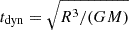 , for the bulk of the interior is less than 10 s. The outer few per cent of the mass of the runaway that was accreted from SN ejecta is more inflated and has a longer dynamical timescale of the order of 100 s, but as we will show, most of this material will quickly become unbound.
Since MESA is a 1D evolutionary code, we averaged the 3D profiles from AREPO over spherical shells defined with respect to the centre of mass of the surviving bound donor. In the case of directly modelling the evolution of the runaway remnant from the AREPO model, we can use the MESA relaxation methods to initialise a WD model directly to the entropy and composition profile specified by the final state of the AREPO model. As we only have one simulation, we also developed an approximate generalised model to account for shock heating in MESA WD models of other masses. The benefit of our method is that we can use the same heating method for multiple white dwarfs of different masses.
To calculate the input heat required to achieve the desired entropy change, we first calculate the entropies of the AREPO white dwarfs (we call the secondary white dwarf a donor before the supernova and a runaway star after the supernova). We specifically start from the AREPO profiles of temperature, density, and composition. From them we compute entropy profiles using PyMesa (Farmer & Bauer 2018) to evaluate the EOS entropy as a function of density, temperature, and composition. We set the equation of state as HELM (Timmes & Swesty 2000) everywhere within the star, consistent with the EOS used in the AREPO simulations. The middle panel in Figure 3 shows the entropy profiles of the donor white dwarf before and after the supernova, and the difference in entropy which can be provided in MESA as a heating term.
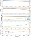 |
Fig. 3. Comparison of different profiles of donor and runaway, and the resulting heating. From top to bottom: first panel Density profiles of the donor (blue) and runaway star (orange). Second panel: Temperature profiles of the donor and the runaway. Third panel: Entropy profiles of the donor and the runaway. Fourth panel: Non-adiabatic heating done after the ejecta hits. Fifth panel: Mass fractions of 12C (similar to 16O), 4He, and 56Ni. The mass coordinates, given in solar masses, are shown until the donor mass of 0.661 M⊙, as outside of this mass range the entropy difference is not defined. The dashed black line represents the mass coordinate where 12C and 16O mass fractions become less than 90% of the total mass fraction. The solid black line shows where the surface cut as defined in Section 2.2.1 is done. The grey portion for helium marks what we remove in our standard models. |
For a given amount of input heat δQ, the first law of thermodynamics states that the entropy and energy will change according to δQ = TdS = dE + PdV. Our goal is to achieve the same non-adiabatic heating profile TΔs represented by the hydrodynamics of the AREPO model. For the case when temperature profiles of our MESA models and the AREPO model are roughly equal (as will be the case for the modelling in this work), we can apply the following heating term to achieve the desired entropy change:
 (1)
(1)
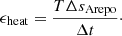
According to the first law of thermodynamics, with specific heating rate ϵheat = δq/δt (where q is heat Q per unit mass), the entropy change Δs achieved for a MESA model over a time period of Δt is then
 (2)
(2)
and using the heating term defined in Equation (1) in Equation (2) then verifies that the total entropy change will be Δs = ΔsArepo, as desired. We verify that this heating approach produces the desired final entropy profile in our MESA models in the next section.
The heating method is similar to one applied in Bauer et al. (2019) for subdwarfs, where an entropy profile is reached by heating up the MESA model. Unlike the Athena++ simulations used in Bauer et al. (2019), the AREPO simulations of Pakmor et al. (2022) track the composition evolution of the donor and include some amount of accreted supernova ejecta as part of the final bound remnant runaway. Therefore, we use the MESA composition relaxation to relax our models to the AREPO composition profiles first, and then heat them up using the other_energy hook in MESA. For all evolution and relaxation scenarios, we use the approx21_plus_co56 nuclear network. This includes the isotopes 1H, 3, 4He, 12C, 14N, 16O, 20Ne, 24Mg, 28Si, 32S, 36Ar, 40Ca, 44Ti, 48, 56Cr, 52, 54, 56Fe, 56Co, and 56Ni. For our purpose the network therefore includes the most important reactions of nickel decay and α capture on carbon.
2.2.1. Direct relaxation versus heating
We first test the heating approach by comparing our heated model to the relaxed one for the case where we can apply both procedures. This comparison requires three steps. First, we start by creating white dwarfs following the test suite template make_co_wd in MESA. We then relax them to the donor profile and the remnant profile of the AREPO simulation. In the second step, we heat the donor white dwarf and compare the state after heating to the runaway white dwarf. In the final step, we compare the evolutionary tracks over 100 Myr of evolution (discussed in Appendix A).
We found it difficult at this stage to evolve models with significant amounts of 56Ni on the surface in MESA due to limitations in the EOS for regions with large fractions of high atomic number elements at low temperature. However, examining the overall energy scales at the surface reveals that the energy input from decay of 56Ni will quickly unbind much of the surface 56Ni on short timescales as soon as the heating from this decay can begin (Shen & Schwab 2017). We therefore estimated an outer layer from which we can confidently remove this 56Ni-dominated material as unbound to make the MESA model easier to evolve, while leaving enough of the outer accreted 56Ni, so that we will still see a residual outflow from nuclear decay energy at early times in our models. For this purpose, we defined an outer boundary for the bound material as the mass coordinate of the fluid element where the energy release due to 56Ni decay is twice the binding energy due to gravity. Gravitational binding energy (per unit mass) is defined as Gm/r, while we estimated Ni decay energy as (5.38 MeV)XNi/(56mp) from the total energy of the decay chain 56Ni → 56Co → 56Fe. This yields a final mass of 0.64 M⊙, where 0.021 M⊙ is the mass lost due to our surface cut. Out of this, we go from having 0.015 M⊙ to ≈0.003 M⊙ of nickel. The binding energy and the decay energy is shown in Figure 4 along with the surface cut allowing us to relax the WD successfully. The remaining 56Ni will still deposit enough radioactive decay energy to drive a residual outflow, as shown in the next section.
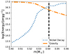 |
Fig. 4. Comparison of 56Ni decay and the gravitational binding energy. The black dashed line marks our choice for the surface cut, where the decay energy is twice the amount of binding energy. |
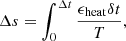
For the second step, we provide the input heat as calculated in Equation (1) over an interval of 0.01 seconds to the relaxed donor WD. During the heating we turned off nuclear burning and mixing. We stopped the evolution of the heated model after the desired amount of heating had been injected to compare to the results from the direct relaxation method. Figure 5 shows the entropy and local thermal diffusion time profiles for the relaxed and heated model. The local thermal diffusion time is given as
 (3)
(3)
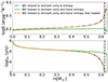 |
Fig. 5. Comparison of heating with relaxation. There are three models here. The blue curve represents the model which has been relaxed to AREPO donor entropy and runaway composition. The orange curve represents the model that has been relaxed to runaway entropy and runaway composition. The green curve represents the blue model, which has been heated. The green and orange overlapping curves show that heating the white dwarf produces the same result as the relaxation. The dashed line marks the layers where the atmosphere is less than 90% C-O dominated, and where an entropy difference is not well defined. |
where H = P/ρg is the local pressure scale height and Dth = 4acT3/3κρ2cP is the coefficient of thermal diffusion.
The dashed black line marks the region where the atmosphere is nickel dominated (defined as the mass fraction of carbon + oxygen less than 90%). Outside this region, the fluid elements do not represent entropy changes from heating, but rather are entirely different fluid elements from regions that were stripped and then replaced by the ejecta. The rest of the star shows almost perfect agreement in the final states. The evolutionary tracks for these models shown in Appendix A also show nearly perfect agreement except for small differences in the first few years of evolution governed by the transient evolution of the very outer layers as they are lost in a super-Eddington wind. The subsequent stellar evolution of these models agrees very well regardless of whether the entropy change is applied through direct relaxation or our heating procedure.
2.2.2. Heating: Other white dwarf masses
Having established that the heating procedure produces a well-defined entropy change, we now explore a wider range of masses. We do this by creating a range of WD donors with core temperatures of 108 K similar to the AREPO donor model. While WD donors in realistic D6 systems may in fact be much cooler than this, these models represent an optimistic assumption about the starting thermal state to which we can add more thermal energy due to supernova interaction. They are therefore a best case scenario for potentially achieving the thermally inflated state observed in D6 runaway candidates. Our white dwarf models are created using make_co_wd in MESA. To create iso-thermal white dwarfs with temperature profiles close to the Arepo profile we turn off thermal neutrino cooling which would otherwise lead to white dwarfs with inverted interior temperature profiles due to thermal neutrino losses in the core. We stop the cooling when the white dwarf reaches a central temperature of 108 K. Our models consist of white dwarfs with final masses of 0.5 M⊙, 0.64 M⊙, 0.85 M⊙, 0.95 M⊙, and 1.1 M⊙, with temperature profiles given in Figure 6. The main parameters of these models are given in Table 1.
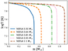 |
Fig. 6. Temperature profiles of all WD models used in this work. |
Relevant mass scales for the different models after the nickel decay cut and for models without helium tail.
All of these models are then relaxed to the composition profile taken directly from the AREPO remnant with a surface cut defined by the 0.64 M⊙ before, scaled to be the same as a function of fractional mass coordinate m/M. Since the mass fractions are assumed to be the same, the total mass of individual elements is scaled by the mass of the model. Furthermore, to heat these models, we use the same ΔsArepo and provide it as a heating term using Equation (1) over a time period of 0.01 s. The maximum timestep is chosen to be 10−4 s, such that a minimum of 100 steps is needed to heat every model. All mixing and nuclear processes are turned off during this step.
This generalisation of heating is approximate since we only have one simulation to rely on. For a less massive donor white dwarf, the binary separation before filling the Roche lobe will be greater, leading to a weaker shock. At the same time the less massive white dwarf is easier to perturb. The scaling is therefore non-trivial and not explored precisely here. For a more massive donor, the separation is smaller, but the internal pressure is higher. Analytic estimates using a white dwarf mass-radius relation indicate that the shock heating will be somewhat weaker for the most massive donors, though this relative shock strength scales relatively weakly with mass (Bauer et al. 2019). So we believe that our method leads to a mild overestimate of the net shock heating for the most massive models, but as we will show, in the context of our work this only strengthens our result that shock heating alone is insufficient to explain the thermal state of the observed objects.
Since the mixing of the helium into the deeper layers is physically unrealistic, our main models only consist of white dwarfs relaxed to a composition profile where the helium in the inner 99% of the white dwarf by mass coordinate is replaced with carbon. These models therefore only have surface helium, which is of the order of 6 × 10⁻⁵ M⊙. Discussion about models with the original AREPO composition is provided in the Appendix B.
3. Evolution for observable timescales
We then carried out the subsequent evolution after relaxation/heating up to a maximum age of 100 Myr. We switched on nuclear burning, convection, and thermohaline mixing (Kippenhahn et al. 1980) (since the atmosphere has many heavy elements), as well as super-Eddington winds for mass loss of the energetically unbound material at the surface. The super-Eddington wind attempts to capture the mass loss that is driven by the 0.003 M⊙ of 56Ni decay at earlier times when the luminosity of the star is greater than the Eddington luminosity. The decay energy of 56Ni deposits heat in excess of the binding energy of the outer layers, which tends to drive the envelope to a radiation-dominated super-Eddington state. The super-Eddington winds help provide a simple prescription for removing this mass from the model as a continuous wind until the heat deposited by Ni decay has either been lost or is no longer sufficient to unbind material. The super-Eddington wind in MESA has a mass loss rate that can be defined as a function of the luminosity L and the local escape velocity vesc as
 (4)
(4)
As the model reaches this luminosity, we apply extra pressure on the stellar atmosphere so that the model is able to evolve through the super-Eddington phase without struggling to resolve the atmospheric boundary condition in the radiation-dominated envelope. The pressure is removed after 103 yr and evolution continues normally. We therefore caution that the details of the observables for the early evolution (first ∼thousand years) should be interpreted as only very approximate, while the later details should generally be more reliable. Since we generally expect to compare to observed runaway remnants at least 104 − 106 years after the supernova explosion, this should be sufficient for our purposes. The comparison of relaxation with heating during this phase of evolution is described in Appendix A, while we focus on the main models here.
3.1. Evolution of the 0.64 M⊙ model
We first discuss the case of a 0.64 M⊙ model. This model has a composition similar to that of the AREPO remnant, but without any helium in the inner 99% of the star by mass. The thermal profile of the model is based on the white dwarf evolution in MESA as shown in Figure 6 (see Figure 7).
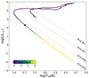 |
Fig. 7. Evolutionary track of the 0.64 M⊙ model. |
The evolution can be broken down into a few major phases. The ρ − T profile evolution is shown in Figure 8 for the 0.64 M⊙ model. As the star is heated the temperature rises and it starts to become less dense. This heating is mostly restricted to the outer layers, and the core remains near the same structure as before. The peak temperature in the model lies near the surface where large amounts of heating occurred. Soon after the initial heating, the decay of 56Ni begins. Figure 9 illustrates the evolution of the mass fractions of different elements at the surface (starting after 3 days). The 56Ni decay causes a super-Eddington wind which puffs up the star causing the density in the outer layers to drop. At the super-Eddington luminosity the star starts to lose mass. While the rest of 56Ni continues to decay, the daughter nuclei of 56Co starts decaying into 56Fe as well. As the half-life of 56Co is larger than 56Ni this process takes slightly longer. However, at the end of only a year of evolution, the surface nickel is gone and the iron content of the surface reaches a maximum. At this point, the star is at its maximum luminosity and radius, while the surface temperature is at a minimum. The net mass loss of this model, along with with the other models is shown in Figure 10.
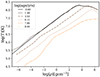 |
Fig. 8. Structural profile of the 0.64 M⊙ model as a function of its age. The puffing up and the later contraction of the star is clearly seen here. The core itself remains relatively unaffected and only the outer layers of the star are affected. |
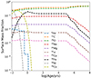 |
Fig. 9. Mass fraction of elements that contribute significantly to the surface composition. The drop in these fractions at the later ages is due to thermohaline mixing. |
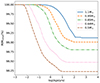 |
Fig. 10. Ratio of mass of the star to its initial mass as a function of its age. There is no mass loss after 103 yr for any model. |
Once all the 56Ni has decayed into 56Fe, the star readjusts thermally over a timescale of 100 years. At this point, the mass loss rate starts to drop and the star begins to contract again. The surface elements, mainly those heavier than carbon and oxygen are mixed inside due to thermohaline mixing, and the surface eventually becomes C/O dominated1. The absence of Helium is due to the fact that no Helium exists in our model for the inner 99% by mass, and that the region where helium was retained is blown away by nickel-powered winds.
3.2. Evolution of a range of masses
The rest of the white dwarfs evolve in a similar way to the 0.64 M⊙ model. The main difference is in the mass loss at the beginning of the evolution. Figure 10 shows the amount of mass lost by these models over time due to super-Eddington winds. Overall, our models lose anywhere between 1 − 2% of their initial mass. This mass loss happens in the layers which were heavily contaminated by 56Ni. Due to this mass loss the total mass fraction of 56Fe at the end of the evolution is lower than would be expected if all the 56Ni was allowed to decay without any mass loss.
The evolution of surface luminosity, radius, and effective temperature are shown in Figure 11. We also overplot the recent D6 observations. We estimate ages of the observations by assuming that the SN ejection should most likely come from somewhere in the Galactic disk. The maximum ages of J1332, J0546, and J1235 are estimated using t = (z + 1)/vz, where z is there present height above the galactic plane, vz is the velocity in z-direction, and 1 kpc is added as an estimate of the scale height of the thick disk (Li & Zhao 2017). For D6-2 we use the minimum and maximum ages of the supernova remnant associated with it (Shen et al. 2018b). As J0927 is coming towards us, we use minimum and maximum ages of 104 and 107 years respectively.
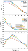 |
Fig. 11. Evolution of the surface luminosity, radius, and temperature of our models. D6 observations are plotted here for the radius. While the radii of D6-1 and D6-3 are similar to those of D6-2, their age estimate is less certain and spans a bigger region. They are not plotted here so as to not overcrowd the diagram. The radius bump at 102 yr for the 1.1 M⊙ is due to a lowering of the extra surface pressure (applied to the early evolution for numerical convergence), and is non-physical. The Teff drop corresponds to this. |
Werner et al. (2024) studied and used NLTE models for spectral fitting of the hottest stars from El-Badry et al. (2023). However, they used cooling tracks of post-AGB stars to get other parameters like the mass, radius, and luminosity. Since, the D6 stars do not fit into this evolutionary channel, we used the radii from El-Badry et al. (2023) instead, but base our uncertainties taking the previous work of Werner et al. (2024) into account. For J332, which is the star closest to the white dwarf cooling track, we used the gravity from Werner et al. (2024), and calculate the uncertainties in the radius assuming a mass distribution from 0.5 − 1.1 M⊙. We adapted the parameters for the original 3 cool D6 candidate stars from the work of Chandra et al. (2022) and Shen et al. (2018a).
This figure again shows the initial puffing up due to the heating and the subsequent nickel decay. However, like before, this mass loss only lasts for a few hundreds of years, after which only iron is left behind. The models reach the cooling track quickly. As their luminosities are relatively high at a radii of 0.01 R⊙, they are also quite hot (> 105 K). Only J1332 is consistent with our models. Every other observation lies outside of our evolutionary tracks due to their inflated nature.
4. Discussion of results and comparison with observations
We compare our models to observed D6 runaway candidates in this section.
4.1. Evolutionary diagrams
The HR and Kiel diagrams of all the models are shown in Figure 12, with the D6 observations over-plotted. We took the temperatures and gravities of the three hottest stars from Werner et al. (2024), from El-Badry et al. (2023) for J1235, and from Chandra et al. (2022) for the cooler D6-1, 2, 3. We calculated the luminosity using
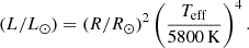 (5)
(5)
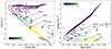 |
Fig. 12. Evolutionary tracks for all WD models. Left panel: HR diagram for all WD models. All observed D6 stars are plotted as black points. The dashed red lines represent the lines of constant radii. The colour bar shows the log(age) of the star. The arrows mark the points when the model is 104 years old. Right panel: Kiel diagram for the same model. The high uncertainty in J0546 comes from combining the minimum and maximum values from Werner et al. (2024) and El-Badry et al. (2023), which have different ways of measuring the radius that lead to inconsistent results. |
The Kiel diagram shows clearly that none of the stars, except J1332, can be explained by our models. For the case of J1332, our models suggest that the star is consistent with being on the cooling track. This was also reported by Werner et al. (2024), who classified this star as a DA-white dwarf. Our result is also in agreement with the mid-plane age (time taken by the star to reach its present height above plane assuming ejection in the disk at z = 0 kpc) of this star calculated by El-Badry et al. (2023) of around 0.6 Myr. For J0546, whose mid-plane age is also similar, the uncertainties are big enough that no conclusion can be reached. The slight overlap of this star with our tracks is possibly due to an overestimation of the uncertainties. That the lower limit of the gravity of the star is overestimated can be seen by the fact that if the star were younger than 103 yr, a supernova remnant would be observable. Furthermore, such a supernova event would have been seen within the recorded history of human civilisation. As no such record exists, it is highly unlikely that the star is so young as a runaway.
4.2. Masses and radii
One of the main aims of this study was to map the AREPO profile of the surviving white dwarf from our single explosion simulation to multiple donor masses. The subsequent evolution for all models showed similar evolutionary tracks, with only the time spent in the super-Eddington luminosity regime being different.
Although we start with relatively hot and luminous white dwarfs in our models, which is inconsistent with searches for runaway stars in supernova remnants (Kerzendorf et al. 2013, 2014, 2018; Shields et al. 2022, 2023), our models do not puff up to match recent observations. Our models all tend toward radii of the order of 0.01 R⊙ within a few thousand years, where their high luminosities lead to the high surface temperatures of our stars (> 105 K). While temperatures close to this have been observed for the hottest D6 stars, many of the observed D6 stars instead have much larger radii and cooler surface temperatures (6000 − 7000 K), which our models are currently unable to explain. As shown by the radial evolution in the middle panel of Figure 11, only 1 star, J1332 is close to the predicted stellar radius.
Table 2 shows the estimated orbital velocities that a donor would have for our models and Table 3 shows the estimated masses for the observed stars based on observed velocities. For D6-1, D6-3, J1235, J0927 the estimated masses are near or above 1 M⊙. For all of the stars except D6-2, the maximum mass within 1σ uncertainties is more than 1.1 M⊙, and especially for the fastest ones is even greater than 1.2 M⊙. Shen et al. (2024) recently pointed out that donor stars less massive than about 1.0 M⊙ may also support double detonations that could destroy the donor in addition to the accretor and produce no runaway, while more massive donors may be more likely to survive and produce a runaway. This may offer an explanation for why the observed candidates tend to have runaway velocities well above 2000 km s−1. At the same time, our 1.1 M⊙ model has the most compact radius and is the farthest away from the observations. J1332 might be explained by our models greater than or equal to 0.85 M⊙, while J0546 cannot be completely ruled out.
Approximate orbital velocities of donors before the supernova.
Ejection velocities with 1σ uncertainties of D6 candidate runaways.
4.3. Thermal time and shock
One of the main results of our work is to show that a supernova shock combined with a deposition of heavy elements like nickel is not enough to explain the parameters of the observed D6 white dwarfs with our current understanding of stellar physics. We show this directly in Figure 13. We plot the ratio of input heat and the internal energy of the white dwarf as a function of the mass coordinate for 0.64 M⊙ and 1.1 M⊙ models. The input heat or TΔs is calculated using the difference of entropy of the initial white dwarf and the post-heating white dwarf from AREPO, multiplied by the initial temperature profile of the white dwarf. The internal energy e is the internal energy of the unperturbed white dwarf. The ratio is therefore a metric to highlight the fractional heating that has occurred in the white dwarf model relative to its original structure. The second axis shows the thermal time of these layers, which is the local thermal diffusion timescale, given in Equation (3). We plot the thermal time at different periods of evolution (after heating and ∼102 − 103 years later after mass loss occurred).
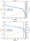 |
Fig. 13. Fraction of input heat and internal energy (left axis, orange), and thermal time (right axis, blue) of the 1.1 M⊙ [top] and 0.64 M⊙ [bottom] models. The dashed and solid black lines represent 10% and 100% of internal energy input as shock heating, respectively. The thermal time is plotted for ages of the order of 0 and > 102 years. |
The plot shows clearly that the input heat due to the supernova shock is too low to significantly perturb the structure and inflate the star in layers of the white dwarf where the thermal time is of the order of the lifetime of the observed D6 white dwarfs. Furthermore, some of the outer layers are eventually stripped away as a result of nickel-powered mass loss. As the white dwarf loses these layers, it decompresses and the thermal time of underlying layers decreases, especially near the surface.
4.4. Opacities, structure, and surface abundances
We have shown above that the shock strength is not enough to perturb the inner regions of a white dwarf and that the thermal time is too short in regions where this shock is high enough. One key limitation of this modelling is that we do not take into account some physics that could influence the precise surface compositions of these runaways at evolutionary times greater than a few thousand years. Thermohaline mixing causes heavy elements to mix deeper into the model and away from the photosphere (see Figure 9), and our modelling does not account for other physics such as element diffusion and radiative levitation that could selectively influence the relative compositions at the photosphere. The resulting surface compositions may impact opacities by orders of magnitude when heavier elements are involved. A significant proportion of iron on the surface, for instance, could lead to unusual opacities. As the radius of the star is dependent on the opacity of different layers, a more precise abundance and opacity calculation is needed. Most candidate spectra show an abundance of lines from heavy elements including C, O, Ne, and Fe, though most have not yet been analysed for detailed surface abundances (Shen et al. 2018a; Chandra et al. 2022; El-Badry et al. 2023). On the other hand, Werner et al. (2024) found that J1332 has a high surface hydrogen and helium abundance. They speculate that this might be the result of J1332 passing through a molecular cloud. Our models show no surface hydrogen or helium on observable timescales, but a conclusive statement can only be made after the exact surface mixing processes are taken into account.
The default MESA opacities are in the form of tables for a given set of composition, temperature, and density from OPAL tables (Iglesias & Rogers 1993), which account for C/O enrichment for high-Z compositions assumed to be ashes of He burning. For our WD models, the surface is polluted with heavier elements due to the supernova ejecta, and no pre-computed opacity tables are available that accurately reflect the unusual surface composition of our initial models. However, there are no noticeable differences between the tabulated opacities and our model opacities at times more than a few 1000 yr because the surface has again become dominated by C/O due to mixing. The surface opacity rises as the effective temperature drops, as seen in Figure 14. As the white dwarf gets older and cools back down the carbon, oxygen, and iron opacities increase. A model which better captures surface mixing, and includes a better model of diffusion and radiative levitation might have a different composition at the surface at later times than what we find. A proper study of these mixing processes was outside of the scope of this work, but is important for any future studies on this topic.
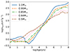 |
Fig. 14. Surface opacity of the star as a function of its age. Surface opacities increase by orders of magnitude as the star cools down the slightly different behaviour of the 1.1 M⊙ model in the beginning is due to the extra pressure applied to evolve during the super-Eddington phase. |
5. Conclusions
In this paper we present results for the first time of 1D stellar evolution of a D6 runaway star produced from a simulation of the D6 supernova detonation scenario. We used composition and temperature-density profiles of the white dwarf from previously published hydrodynamical simulations of WD binary supernovae made in AREPO. We were able to map these into MESA and heat white dwarfs representing donors in the mass range 0.5 M⊙−1.1 M⊙. We then evolved these models to 100 Myr after the supernova explosion.
Our work clearly shows that with our current understanding of the physics of stellar structure for these models, the post-supernova explosion shock is not enough to explain runaway observations. Our WD donor models have very high interior temperatures of 108 K, which would correspond to a cooling age of no more than a few megayears for normal WDs, representing a maximally optimistic choice for their starting thermal state. Despite this, the white dwarfs do not heat and expand for a timescale which matches the observed inflated D6 stars. The only star which lies on our evolutionary tracks is J1332, which has possibly been a runaway long enough to return back to the white dwarf cooling track. Our results show that the stars spend only few hundred years puffed up to around 0.1 R⊙, powered by the decay of 56Ni and shock heating of their outer layers. The significant radioactive heating at the surface from nickel decay leads to most of the accreted supernova ejecta being quickly lost again as a wind, and does not appear to produce heating that can penetrate deeper into the core. After all the nickel has been converted to iron and after the luminosity returns back to sub-Eddington, the white dwarf starts to cool down, but always having reached a compact structure on the WD cooling track for our models.
This modelling contrasts with previous more successful attempts to explain inflated states of runaways from hot subdwarf donors (Bauer et al. 2019) or bound Iax remnants (Zhang et al. 2019), for which some models are able to reach unusual inflated states for megayear timescales. However, only a WD donor can explain the observed velocities for many of the hypervelocity runaways now being discovered. Unlike the hot subdwarf or Iax scenarios, in the case of WD donors in D6 binaries, the central pressure of the donor WD is much greater compared to the shock driven by SN interaction. Therefore, the shock that traverses the core of the donor is relatively weak and unable to significantly perturb its thermal structure. Significant heating is largely confined to superficial layers with short thermal timescales near the surface, and these layers are either quickly lost through winds or able to thermally readjust and settle back into a compact configuration over timescales much shorter than 1 Myr in our models. Explaining the unusually inflated states of many of the observed high-velocity runaways requires either (1) an additional source of significant heating or (2) additional physics influencing the structure and evolution that is not currently accounted for in our modelling.
While our work has focused on the long-term evolution of the structure of the white dwarf, the next step in refining this modelling will be precise modelling of the surface abundances. Our thermohaline mixing prescription shows that the heavier elements sink down into the white dwarf such that surface abundance of these stars eventually becomes dominated by carbon and oxygen dredged from the core. A better prescription of diffusion and radiative levitation which acts on the heavier elements like iron and changes surface composition should be investigated in the future. Furthermore, 3 dimensional hydrodynamical simulations dealing with the most massive donors should also be investigated for a better understanding of the post-supernova shock heating to improve upon our current approximate scaling based on just one detailed simulation of a 0.7 M⊙ WD donor.
Data availability
The MESA input files and inlists for relaxation, heating, and evolution can be accessed at https://doi.org/10.5281/zenodo.13477859
Due to a limitation from the tabulated EOS used for the lowest density outer layers, the MESA thermohaline prescription does not recognise that thermohaline instability should occur for Fe lying on top of the C/O core (because the tabulation in terms of metallicity Z does not recognise these as different). We therefore apply a minimal amount of mixing in the outer few per cent of the mass of the star, which connects the Fe in these outer layers to the thermohaline mixing in the deeper core where the EOS resolves these differences, and therefore adequately captures the net effect of global interior thermohaline mixing pulling the heavy Fe away from the atmosphere.
Acknowledgments
This project was originally started as part of the Kavli Summer Program which took place in the Max Planck Institute for Astrophysics in Garching in July 2023, supported by the Kavli Foundation. We are grateful to Stephen Justham, Selma de Mink, and Jim Fuller for enriching discussions. We would like to thank the anonymous referee for their helpful report. A.B. was supported by the Deutsche Forschungsgemeinschaft (DFG) through grant GE2506/18-1. K.J.S. was supported by NASA through the Astrophysics Theory Program (80NSSC20K0544) and by NASA/ESA Hubble Space Telescope programs #15871 and #15918. W.E.K. was supported by NSF Grants OAC-2311323, AST-2206523, and NASA/ESA HST-AR-Theory HST-AR-16613.002-A. K.E. was supported in part by HST-GO-17441.001-A. AB and ASR would like to thank Rob Farmer for his support with PyMESA.
References
- Angulo, C., Arnould, M., Rayet, M., et al. 1999, Nucl. Phys. A, 656, 3 [Google Scholar]
- Bauer, E. B., White, C. J., & Bildsten, L. 2019, ApJ, 887, 68 [Google Scholar]
- Bauer, E. B., Chandra, V., Shen, K. J., & Hermes, J. J. 2021, ApJ, 923, L34 [NASA ADS] [CrossRef] [Google Scholar]
- Boos, S. J., Townsley, D. M., Shen, K. J., Caldwell, S., & Miles, B. J. 2021, ApJ, 919, 126 [NASA ADS] [CrossRef] [Google Scholar]
- Boos, S. J., Townsley, D. M., & Shen, K. J. 2024, ApJ, 972, 200 [NASA ADS] [CrossRef] [Google Scholar]
- Cassisi, S., Potekhin, A. Y., Pietrinferni, A., Catelan, M., & Salaris, M. 2007, ApJ, 661, 1094 [NASA ADS] [CrossRef] [Google Scholar]
- Chandra, V., Hwang, H.-C., Zakamska, N. L., et al. 2022, MNRAS, 512, 6122 [CrossRef] [Google Scholar]
- Chugunov, A. I., Dewitt, H. E., & Yakovlev, D. G. 2007, Phys. Rev. D, 76, 025028 [NASA ADS] [CrossRef] [Google Scholar]
- Cyburt, R. H., Amthor, A. M., Ferguson, R., et al. 2010, ApJS, 189, 240 [NASA ADS] [CrossRef] [Google Scholar]
- Dan, M., Rosswog, S., Guillochon, J., & Ramirez-Ruiz, E. 2011, ApJ, 737, 89 [NASA ADS] [CrossRef] [Google Scholar]
- Dan, M., Rosswog, S., Guillochon, J., & Ramirez-Ruiz, E. 2012, MNRAS, 422, 2417 [NASA ADS] [CrossRef] [Google Scholar]
- El-Badry, K., Shen, K. J., Chandra, V., et al. 2023, Open J. Astrophys., 6, 28 [CrossRef] [Google Scholar]
- Farmer, R., & Bauer, E. B. 2018, rjfarmer/pyMesa: Add support for 10398, https://doi.org/10.5281/zenodo.1205271 [Google Scholar]
- Ferguson, J. W., Alexander, D. R., Allard, F., et al. 2005, ApJ, 623, 585 [Google Scholar]
- Fink, M., Hillebrandt, W., & Röpke, F. K. 2007, A&A, 476, 1133 [NASA ADS] [CrossRef] [EDP Sciences] [Google Scholar]
- Fuller, G. M., Fowler, W. A., & Newman, M. J. 1985, ApJ, 293, 1 [NASA ADS] [CrossRef] [Google Scholar]
- Geier, S., Fürst, F., Ziegerer, E., et al. 2015, Science, 347, 1126 [Google Scholar]
- Guillochon, J., Dan, M., Ramirez-Ruiz, E., & Rosswog, S. 2010, ApJ, 709, L64 [Google Scholar]
- Hills, J. G. 1988, Nature, 331, 687 [Google Scholar]
- Hirsch, H. A., Heber, U., O’Toole, S. J., & Bresolin, F. 2005, A&A, 444, L61 [NASA ADS] [CrossRef] [EDP Sciences] [Google Scholar]
- Iglesias, C. A., & Rogers, F. J. 1993, ApJ, 412, 752 [Google Scholar]
- Iglesias, C. A., & Rogers, F. J. 1996, ApJ, 464, 943 [NASA ADS] [CrossRef] [Google Scholar]
- Irwin, A. W. 2004, The FreeEOS Code for Calculating the Equation of State for Stellar Interiors, http://freeeos.sourceforge.net [Google Scholar]
- Itoh, N., Hayashi, H., Nishikawa, A., & Kohyama, Y. 1996, ApJS, 102, 411 [NASA ADS] [CrossRef] [Google Scholar]
- Jermyn, A. S., Schwab, J., Bauer, E., Timmes, F. X., & Potekhin, A. Y. 2021, ApJ, 913, 72 [NASA ADS] [CrossRef] [Google Scholar]
- Jermyn, A. S., Bauer, E. B., Schwab, J., et al. 2023, ApJS, 265, 15 [NASA ADS] [CrossRef] [Google Scholar]
- Kerzendorf, W. E., Yong, D., Schmidt, B. P., et al. 2013, ApJ, 774, 99 [NASA ADS] [CrossRef] [Google Scholar]
- Kerzendorf, W. E., Childress, M., Scharwächter, J., Do, T., & Schmidt, B. P. 2014, ApJ, 782, 27 [NASA ADS] [CrossRef] [Google Scholar]
- Kerzendorf, W. E., Strampelli, G., Shen, K. J., et al. 2018, MNRAS, 479, 192 [NASA ADS] [CrossRef] [Google Scholar]
- Kippenhahn, R., Ruschenplatt, G., & Thomas, H. C. 1980, A&A, 91, 175 [Google Scholar]
- Kromer, M., Sim, S. A., Fink, M., et al. 2010, ApJ, 719, 1067 [Google Scholar]
- Langanke, K., & Martínez-Pinedo, G. 2000, Nucl. Phys. A, 673, 481 [NASA ADS] [CrossRef] [Google Scholar]
- Lawlor, T. M., & MacDonald, J. 2006, MNRAS, 371, 263 [NASA ADS] [CrossRef] [Google Scholar]
- Li, C., & Zhao, G. 2017, ApJ, 850, 25 [NASA ADS] [CrossRef] [Google Scholar]
- Moll, R., & Woosley, S. E. 2013, ApJ, 774, 137 [NASA ADS] [CrossRef] [Google Scholar]
- Oda, T., Hino, M., Muto, K., Takahara, M., & Sato, K. 1994, At. Data Nucl. Data Tab., 56, 231 [NASA ADS] [CrossRef] [Google Scholar]
- Pakmor, R., Kromer, M., Taubenberger, S., & Springel, V. 2013, ApJ, 770, L8 [Google Scholar]
- Pakmor, R., Springel, V., Bauer, A., et al. 2016, MNRAS, 455, 1134 [Google Scholar]
- Pakmor, R., Callan, F. P., Collins, C. E., et al. 2022, MNRAS, 517, 5260 [NASA ADS] [CrossRef] [Google Scholar]
- Paxton, B., Bildsten, L., Dotter, A., et al. 2011, ApJS, 192, 3 [Google Scholar]
- Paxton, B., Cantiello, M., Arras, P., et al. 2013, ApJS, 208, 4 [Google Scholar]
- Paxton, B., Marchant, P., Schwab, J., et al. 2015, ApJS, 220, 15 [Google Scholar]
- Paxton, B., Schwab, J., Bauer, E. B., et al. 2018, ApJS, 234, 34 [NASA ADS] [CrossRef] [Google Scholar]
- Paxton, B., Smolec, R., Schwab, J., et al. 2019, ApJS, 243, 10 [Google Scholar]
- Poutanen, J. 2017, ApJ, 835, 119 [NASA ADS] [CrossRef] [Google Scholar]
- Raddi, R., Hollands, M. A., Koester, D., et al. 2018, ApJ, 858, 3 [NASA ADS] [CrossRef] [Google Scholar]
- Raddi, R., Hollands, M. A., Koester, D., et al. 2019, MNRAS, 489, 1489 [Google Scholar]
- Schwab, J., Shen, K. J., Quataert, E., Dan, M., & Rosswog, S. 2012, MNRAS, 427, 190 [NASA ADS] [CrossRef] [Google Scholar]
- Shen, K. J., & Schwab, J. 2017, ApJ, 834, 180 [NASA ADS] [CrossRef] [Google Scholar]
- Shen, K. J., Bildsten, L., Kasen, D., & Quataert, E. 2012, ApJ, 748, 35 [Google Scholar]
- Shen, K. J., Boubert, D., Gänsicke, B. T., et al. 2018a, ApJ, 865, 15 [Google Scholar]
- Shen, K. J., Kasen, D., Miles, B. J., & Townsley, D. M. 2018b, ApJ, 854, 52 [Google Scholar]
- Shen, K. J., Boos, S. J., & Townsley, D. M. 2024, ApJ, 975, 127 [NASA ADS] [CrossRef] [Google Scholar]
- Shields, J. V., Kerzendorf, W., Hosek, M. W., et al. 2022, ApJ, 933, L31 [NASA ADS] [CrossRef] [Google Scholar]
- Shields, J. V., Arunachalam, P., Kerzendorf, W., et al. 2023, ApJ, 950, L10 [NASA ADS] [CrossRef] [Google Scholar]
- Springel, V. 2010, MNRAS, 401, 791 [Google Scholar]
- Tanikawa, A., Nomoto, K., Nakasato, N., & Maeda, K. 2019, ApJ, 885, 103 [NASA ADS] [CrossRef] [Google Scholar]
- Timmes, F. X., & Swesty, F. D. 2000, ApJS, 126, 501 [NASA ADS] [CrossRef] [Google Scholar]
- Vennes, S., Nemeth, P., Kawka, A., et al. 2017, Science, 357, 680 [Google Scholar]
- Weinberger, R., Springel, V., & Pakmor, R. 2020, ApJS, 248, 32 [Google Scholar]
- Werner, K., Reindl, N., Rauch, T., El-Badry, K., & Bédard, A. 2024, A&A, 682, A42 [NASA ADS] [CrossRef] [EDP Sciences] [Google Scholar]
- Wong, T. L. S., White, C., & Bildsten, L. 2024, ApJ, 973, 65 [NASA ADS] [CrossRef] [Google Scholar]
- Zhang, M., Fuller, J., Schwab, J., & Foley, R. J. 2019, ApJ, 872, 29 [Google Scholar]
Appendix A: Comparing the relaxed and heated Arepo remnant
We show evolutionary tracks in the HR diagram for the 0.64 M⊙ model mapped directly from Arepo in the left panel of Figure A.1. The bump in luminosity and radius at around 3 × 10⁴ years occurs due to unstable burning of helium in both relaxed and heated cases. As we do not think the presence of helium is physically realistic, we also show a comparison with the model without any helium in the inner regions in the right panel of Figure A.1.
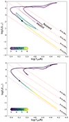 |
Fig. A.1. HR diagrams for the 0.64 M⊙ model. [Top Panel] Evolutionary track of the 0.64 M⊙ model relaxed directly to the remnant profile and the model relaxed to donor profile and then heated. Red lines show lines of constant radii from 0.01 − 0.3 R⊙. Only ∼0.001% of the total evolutionary time is spent above R > 0.03 R⊙, without considering the helium flash. [Bottom Panel] Comparison plot of the model without any helium in the inner layers of the star. |
Both the relaxed and heated remnant models reach a similar state quickly. We show the evolution of stellar surface quantities in Figure A.2. There are no significant differences between the two models. For the model without helium inside, the track converges to the same state as the other models after a few megayears. The models reach super-Eddington luminosity due to heating and Nickel decay within a few days. The Eddington limit is reached within the first year but declines quickly after the first 100 years. The star briefly inflates to a large radius, but this state is short-lived. The bumps in all three quantities after 104 yr for the first two models are due to a helium flash. Those models ignite this helium at the same time, confirming that the initial states are the same for the relaxation and heating. This is not seen for the model without helium in the inner 99% of the star.
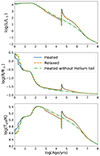 |
Fig. A.2. Evolution of surface luminosity, radius, and effective temperature of the heated (blue) and relaxed (orange) models for comparison. Also plotted are the quantities for the heated model without any helium in the inner regions of the star (green). |
This comparison shows that heating the model provides the same result as a direct relaxation, in the case when the compositions are the same, and the heat is calculated as a difference of entropy from the AREPO model. We therefore are able to generalise the heating procedure and rely on it for the evolution of the bigger grid of models. Insofar as the temperature profiles of the white dwarfs are roughly the same, this method can be applied to a model of any mass. Furthermore the end state of the relaxed model is the same as the end state of the helium-less heated model, except for a short-lived loop in the HR diagram. After a few thousand years both of these models are in the same region of the HR diagram.
Appendix B: Models with AREPO composition
The HR diagram of all the models with Arepo composition (no re-scaling of helium) is shown in Figure B.1, with the D6 observations over-plotted. These models have a total of around 0.002 M⊙ of Helium.
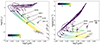 |
Fig. B.1. Evolutionary tracks for all WD models without any helium removed. [left panel] HR diagram for grid 1 models. All reported D6 stars are plotted as black points. Red lines represent lines of constant radii. The colour bar shows the log(age) of the star. [right panel] Kiel diagram for the same model. The high uncertainty in J3546 comes from combining the minimum and maximum values from Werner et al. (2024) and El-Badry et al. (2023). The big loop of 0.50 M⊙ and the smaller loop of 0.64 M⊙ models is due to unstable helium burning. |
The HR diagram of all models is similar to the models without helium discussed before. All stars spend < 104 yr at high luminosities, by which time the Nickel decay is quenched and the star has lost some mass due to radiation powered winds. After this time the stars continue to burn helium stably, and reach the tip of the white dwarf cooling track. There is only one model where the helium flash occurs. However, since this only occurs in the lowest mass WD, it should not be considered as an explanation for the observed stars. This is especially because the D6 stars lying on this region of the HR diagram should have been high-mass (> 0.8 M⊙) donors (Bauer et al. 2021). This instability is also dependent on the initial structure of the chosen model, as the 0.64 M⊙ model does not have a strong helium flash in this case (as opposed to the relaxed models before). For a better comparison with spectral results, we also show the Kiel diagram in right panel of Figure B.1.
The evolution of surface luminosity, radius, and temperature are shown in Figure B.2. We also plot regions of estimated radii of known D6 stars for an age between 104 − 107 yr. The fact that two D6 stars coincide with the radii of the 0.5 M⊙ model is again due to the helium flash and should not be considered as a confirmation of the models.
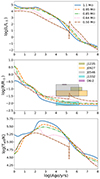 |
Fig. B.2. Evolution of the luminosity, radius, and temperature of models with AREPO helium content. |
All Tables
Relevant mass scales for the different models after the nickel decay cut and for models without helium tail.
All Figures
|
Fig. 1. Main elements and their composition profiles as a function of radius for the donor right before the supernova [top] and the runaway 150 s after the supernova [bottom] for mass coordinates, which remain bound after supernova explosion (< 0.661 M⊙). In particular, 56Ni dominates the mass fraction at the surface of the runaway. The surface helium content of the donor is less than 0.03 M⊙ as most of it has been accreted by the primary. |
| In the text | |
|
Fig. 2. Mass fraction of helium in the donor at two different times. Top panel: Helium mass fraction at the beginning of the simulation showing no mixing. Bottom panel: Mixing of helium in the donor just before the explosion of the accretor. The red line shows a contour of ρ = 104 g cm−3. During the accretion and inspiral the helium from the surface seeps into the deeper layers of the donor. |
| In the text | |
|
Fig. 3. Comparison of different profiles of donor and runaway, and the resulting heating. From top to bottom: first panel Density profiles of the donor (blue) and runaway star (orange). Second panel: Temperature profiles of the donor and the runaway. Third panel: Entropy profiles of the donor and the runaway. Fourth panel: Non-adiabatic heating done after the ejecta hits. Fifth panel: Mass fractions of 12C (similar to 16O), 4He, and 56Ni. The mass coordinates, given in solar masses, are shown until the donor mass of 0.661 M⊙, as outside of this mass range the entropy difference is not defined. The dashed black line represents the mass coordinate where 12C and 16O mass fractions become less than 90% of the total mass fraction. The solid black line shows where the surface cut as defined in Section 2.2.1 is done. The grey portion for helium marks what we remove in our standard models. |
| In the text | |
|
Fig. 4. Comparison of 56Ni decay and the gravitational binding energy. The black dashed line marks our choice for the surface cut, where the decay energy is twice the amount of binding energy. |
| In the text | |
|
Fig. 5. Comparison of heating with relaxation. There are three models here. The blue curve represents the model which has been relaxed to AREPO donor entropy and runaway composition. The orange curve represents the model that has been relaxed to runaway entropy and runaway composition. The green curve represents the blue model, which has been heated. The green and orange overlapping curves show that heating the white dwarf produces the same result as the relaxation. The dashed line marks the layers where the atmosphere is less than 90% C-O dominated, and where an entropy difference is not well defined. |
| In the text | |
|
Fig. 6. Temperature profiles of all WD models used in this work. |
| In the text | |
|
Fig. 7. Evolutionary track of the 0.64 M⊙ model. |
| In the text | |
|
Fig. 8. Structural profile of the 0.64 M⊙ model as a function of its age. The puffing up and the later contraction of the star is clearly seen here. The core itself remains relatively unaffected and only the outer layers of the star are affected. |
| In the text | |
|
Fig. 9. Mass fraction of elements that contribute significantly to the surface composition. The drop in these fractions at the later ages is due to thermohaline mixing. |
| In the text | |
|
Fig. 10. Ratio of mass of the star to its initial mass as a function of its age. There is no mass loss after 103 yr for any model. |
| In the text | |
|
Fig. 11. Evolution of the surface luminosity, radius, and temperature of our models. D6 observations are plotted here for the radius. While the radii of D6-1 and D6-3 are similar to those of D6-2, their age estimate is less certain and spans a bigger region. They are not plotted here so as to not overcrowd the diagram. The radius bump at 102 yr for the 1.1 M⊙ is due to a lowering of the extra surface pressure (applied to the early evolution for numerical convergence), and is non-physical. The Teff drop corresponds to this. |
| In the text | |
|
Fig. 12. Evolutionary tracks for all WD models. Left panel: HR diagram for all WD models. All observed D6 stars are plotted as black points. The dashed red lines represent the lines of constant radii. The colour bar shows the log(age) of the star. The arrows mark the points when the model is 104 years old. Right panel: Kiel diagram for the same model. The high uncertainty in J0546 comes from combining the minimum and maximum values from Werner et al. (2024) and El-Badry et al. (2023), which have different ways of measuring the radius that lead to inconsistent results. |
| In the text | |
|
Fig. 13. Fraction of input heat and internal energy (left axis, orange), and thermal time (right axis, blue) of the 1.1 M⊙ [top] and 0.64 M⊙ [bottom] models. The dashed and solid black lines represent 10% and 100% of internal energy input as shock heating, respectively. The thermal time is plotted for ages of the order of 0 and > 102 years. |
| In the text | |
|
Fig. 14. Surface opacity of the star as a function of its age. Surface opacities increase by orders of magnitude as the star cools down the slightly different behaviour of the 1.1 M⊙ model in the beginning is due to the extra pressure applied to evolve during the super-Eddington phase. |
| In the text | |
|
Fig. A.1. HR diagrams for the 0.64 M⊙ model. [Top Panel] Evolutionary track of the 0.64 M⊙ model relaxed directly to the remnant profile and the model relaxed to donor profile and then heated. Red lines show lines of constant radii from 0.01 − 0.3 R⊙. Only ∼0.001% of the total evolutionary time is spent above R > 0.03 R⊙, without considering the helium flash. [Bottom Panel] Comparison plot of the model without any helium in the inner layers of the star. |
| In the text | |
|
Fig. A.2. Evolution of surface luminosity, radius, and effective temperature of the heated (blue) and relaxed (orange) models for comparison. Also plotted are the quantities for the heated model without any helium in the inner regions of the star (green). |
| In the text | |
|
Fig. B.1. Evolutionary tracks for all WD models without any helium removed. [left panel] HR diagram for grid 1 models. All reported D6 stars are plotted as black points. Red lines represent lines of constant radii. The colour bar shows the log(age) of the star. [right panel] Kiel diagram for the same model. The high uncertainty in J3546 comes from combining the minimum and maximum values from Werner et al. (2024) and El-Badry et al. (2023). The big loop of 0.50 M⊙ and the smaller loop of 0.64 M⊙ models is due to unstable helium burning. |
| In the text | |
|
Fig. B.2. Evolution of the luminosity, radius, and temperature of models with AREPO helium content. |
| In the text | |
Current usage metrics show cumulative count of Article Views (full-text article views including HTML views, PDF and ePub downloads, according to the available data) and Abstracts Views on Vision4Press platform.
Data correspond to usage on the plateform after 2015. The current usage metrics is available 48-96 hours after online publication and is updated daily on week days.
Initial download of the metrics may take a while.