| Issue |
A&A
Volume 693, January 2025
|
|
|---|---|---|
| Article Number | A231 | |
| Number of page(s) | 18 | |
| Section | Planets, planetary systems, and small bodies | |
| DOI | https://doi.org/10.1051/0004-6361/202450719 | |
| Published online | 21 January 2025 | |
Uranus’ hydrogen upper atmosphere: Insights from pre- and post-equinox HST Lyman-α images
1
Royal Institute of Technology (KTH),
Stockholm,
Sweden
2
Southwest Research Institute,
San Antonio,
TX,
USA
3
Central Arizona College,
Coolidge,
AZ,
USA
4
LESIA, Observatoire de Paris, Université PSL, CNRS, Sorbonne Université, Université de Paris,
Meudon,
France
5
Aix Marseille Université, CNRS, CNES, LAM,
Marseille,
France
★ Corresponding author; This email address is being protected from spambots. You need JavaScript enabled to view it.
Received:
14
May
2024
Accepted:
12
November
2024
Abstract
We present the first spatially resolved images of Lyman-α (Lyα) emissions from Uranus taken by the Hubble Space Telescope (HST). The observations were carried out using HST’s Space Telescope Imaging Spectrograph instrument as part of two far-ultraviolet (FUV) observing campaigns in 1998 and 2011, before and after Uranus’ equinox in 2007. The average intensities (± uncertainties) on Uranus’ disk were 860 ± 6 and 725 ± 9 R, respectively. The images reveal widely extended emissions, detectable up to ~4 Uranus radii (RU). We performed simulations of the Lyα radiative transfer in the atmosphere, considering resonant scattering by H, Rayleigh scattering by H2, and absorption by CH4. We considered only solar Lyα fluxes at Uranus as the Lyα source for simulations. The effects of hydrogen in the interplanetary medium and Earth’s exosphere on Uranus’ Lyα emissions were taken into account. We find a good agreement between on-disk brightnesses from simulations and the HST observations assuming the (H, H2, and CH4) atmosphere profile derived from Voyager 2 measurements. Only slight adjustments of the H or H2 densities were required in some of the simulation cases, in particular, for the 1998 observations. To match the off-disk HST brightnesses in both years, a substantial exosphere of gravitationally bound hot H is required, which we modelled assuming the hot H number density has a Chapman profile. We find that compared to 1998, the hot H abundance required for 2011 is lower and the inferred hot H profiles seem to be more extended. This bound hot H is likely to be a persistent part of Uranus’ upper atmosphere and is distinct from the escaping hot H population derived from Voyager 2 observations. We discuss the possible production mechanisms involving solar EUV radiation and study the sensitivity of the modelled brightness to the parameters of the hot H profile. We find that solar EUV radiation is not a sufficient source to explain the hot H in the exosphere of Uranus.
Key words: radiative transfer / methods: numerical / techniques: image processing / interplanetary medium / planets and satellites: atmospheres / planets and satellites: gaseous planets
© The Authors 2025
 Open Access article, published by EDP Sciences, under the terms of the Creative Commons Attribution License (https://creativecommons.org/licenses/by/4.0), which permits unrestricted use, distribution, and reproduction in any medium, provided the original work is properly cited.
This article is published in open access under the Subscribe to Open model. This email address is being protected from spambots. You need JavaScript enabled to view it. to support open access publication.
1 Introduction
Uranus is among the least explored planets in the Solar System, visited only by the Voyager 2 spacecraft during its 1986 flyby. The geometry of the Uranus system is unlike any other planet in the Solar System. Its extreme obliquity of 97.8° and orbital period of 84 years can lead to substantial seasonal forcing of its atmosphere. Moreover, the magnetic axis has a large angle (59°) with respect to the rotation axis, and it is offset by nearly 1/3rd of Uranus radius from its centre. The complex magnetic field topology affects the plasma environment and possibly also the upper atmosphere. At giant planets, the upper atmosphere plays a key role in various processes such as photochemistry, interaction with plasma environment and possibly solar wind’, magnetosphere-ionosphere coupling, atmospheric escape, and interaction with ring particles (e.g. see O’Donoghue & Stallard (2022) and references therein).
As a giant planet, the upper atmosphere of Uranus is primarily composed of atomic and molecular hydrogen (Broadfoot et al. 1986). Several aspects of this upper atmosphere are not well understood. Since atomic hydrogen efficiently scatters Lyman- α (Lyα, 121.567 nm) photons, remote sensing observations at this wavelength provide an excellent tool for studying the upper atmosphere. The first Lyα observations of Uranus were obtained with the International Ultraviolet Explorer (IUE) observatory using its Short Wavelength Spectrograph instrument and were reported by Clarke (1982), Durrance & Moos (1982), and Clarke et al. (1986). From the analysis of these 31 spatially unresolved observations of Uranus taken between March 1982 and September 1985 (see Table 1 from Clarke et al. (1986)), these authors reported minimum, maximum, and average disk-integrated Lyα brightnesses of 790 ± 250, 2590 ± 300, and 1400 ± 450 R, respectively. The average brightness was larger than the expected values determined from the contemporary observations of Jupiter and Saturn. Clarke et al. (1986) attributed aurora as a primary mechanism for these high and variable Lyα emissions from Uranus.
During the Voyager 2 flyby, Uranus was observed from close distances for the first time. From the spatially resolved Voyager 2 Ultraviolet Spectrometer (UVS) observations, Broadfoot et al. (1986) also reported bright Lyα emissions from Uranus, approximately 1500 R near the subsolar point. However, they reported only weak auroral emission of 45 R from the polar regions, contradicting the claims made by earlier studies using IUE observations. They estimated the contribution of 400–500 R from resonant scattering by H in the Voyager 2 Lyα observations.
Broadfoot et al. (1986) explained the remaining ~1000 R Lyα brightness with a controversial mechanism of emissions from H and H2 caused due to excitation by low energy electrons, labelled as an ‘electroglow’. From the UVS observations, Yelle et al. (1987) deduced the presence of H2 Raman scattered Lyα emissions at 1280 Å, with the determined brightness of 40 ± 20 R. From this Raman feature brightness, they determined 200 R to 500 R (of the total brightness of 1500 R) should come from the Rayleigh scattering by H2 of the solar Lyα flux. An important implication of the presence of this 1280 Å Raman line (and thus effective Rayleigh scattering at 1216 Å) was that the upper atmosphere of Uranus is devoid of absorbing hydrocarbons. Uranus is the only gas planet where this Raman feature has been observed, and it seems to be absent for Jupiter, Saturn, and Neptune (Carlson & Judge 1971; Yelle et al. 1987; Broadfoot et al. 1989). With improved radiative transfer modelling for UVS Lyα observations done in studies such as Ben Jaffel et al. (1991) and Emerich et al. (1993), it was later found that the electroglow explanation is probably not required to explain the bright Lyα emissions from giant planets’ upper atmospheres. These two studies present the arguments that previous models had underestimated the contribution of resonant scattering in the Lyα emissions from the giant planets. Instead, these authors estimated that the resonant scattering by H and Rayleigh scattering by H2 was able to explain the majority of the on-disk Lyα emissions observed from the giant planet atmospheres.
Apart from bright Lyα emissions from Uranus’ disk, Voyager 2 revealed a substantial H exosphere above the H2 dominated upper atmosphere, extending to several Uranus radii altitude (Herbert et al. 1987; Herbert & Hall 1996). To explain the far-reaching extent of the H exosphere, Herbert & Hall (1996) suggested the presence of a non-thermal, ‘hot’ population of H with temperature of at least 2 eV along with the thermal H population. Herbert & Sandel (1999) provide a review on the ultraviolet observations of Uranus from IUE, Voyager 2, and pre-1998 Hubble Space Telescope (HST) campaigns, while Strobel et al. (1991) provide a review on the processes occurring in the Uranian upper atmosphere. They argued that the electroglow mechanism could not work in a collisional atmosphere because backscattered electrons would be decelerated by the hypothesised electric field accelerating the electrons. From our understanding of the Lyα emissions of Uranus so far, the major contributors to these emissions are the resonant and Rayleigh scattering of the incident Lyα flux by H and H2, respectively. Furthermore, Rayleigh scattering is efficient due to the low abundance of CH4 or any other hydrocarbon in the upper atmosphere.
After the Voyager 2 flyby, the observational studies advancing the knowledge of Uranus’ atmosphere and magnetosphere used ground- or space-based observatories. HST observations at ultraviolet wavelengths have played a key role in our understanding of the upper atmospheres of giant planets (e.g. see O’Donoghue & Stallard (2022) and references therein). HST observed Uranus in far-ultraviolet (FUV) wavelengths in several campaigns since 1998. Lamy et al. (2012) reported the first Earth-based detection of Uranus’ aurorae from ’HST observations of H2 FUV bands obtained using Space Telescope Imaging Spectrograph (STIS) instrument in July 1998 and November 2011’. Subsequently, Lamy et al. (2017) detected Uranian aurorae in FUV images obtained in two other HST/STIS campaigns, executed in September 2012 and November 2014, while Barthélemy et al. (2014) analysed the H2 FUV spectra in the STIS observations, including those associated with aurora detection from September 2012. In these studies using HST observations, the analysed auroral signatures were observed around both magnetic poles as localised time-variable emissions on the dayside of the Uranian disc. While they unambiguously retrieved the H2 signature in auroral emissions (either through spectra or filters rejecting Lyα), the presence of auroral H Lyα emission in HST observations remains an open question to date. Several other HST Uranus observations, taken at multiple wavelength bands, focused on the lower and middle atmosphere1 and there is a vast potential for a comprehensive study of the upper atmosphere through HST UV observations.
In this study, we analysed FUV observations of Uranus taken in 1998 and 2011 using HST’s STIS instrument with observing campaigns 7439 and 12239, respectively. These observations contain the first spatially resolved images from Earth-orbit of the Lyα emissions from an ice giant planet, and they have not yet been analysed in any published study so far. Uranus went through equinox in 2007, transitioning from southern solstice in 1986 (during Voyager 2 flyby) to northern solstice in 2028. Thus, these observations allow us to probe the state of Uranus’ widely extended neutral upper atmosphere before and after equinox. Analysing such observations taken at different time periods can help us understand how Uranus’ upper atmosphere changes over its orbital period. Two entities of concern for HST Lyα observations of Solar System objects are H in the interplanetary medium (hereafter, IPH) and H in the exosphere of the Earth (hereafter, EEH) (e.g. see Baliukin et al. 2022 and Baliukin et al. 2019 and references therein for IPH and EEH, respectively). IPH and EEH resonantly scatter Lyα radiation. In addition to the planetary Lyα radiation, they also contribute to the Lyα signal recorded by STIS (the scattered solar Lyα photons by EEH are called as H geocorona). Apart from this, IPH and EEH may cause the extinction of Lyα emissions from the Solar System bodies. Thus, it is necessary to analyse the effects of IPH and EEH on Uranus’ Lyα signal seen by HST. In our study, we investigate the Lyα global brightness and spatial distribution of Uranus’ atmosphere observed in the HST STIS images. We did it by radiative transfer modelling of the scattering and absorption processes in the Uranian atmosphere and taking into account the extinction of Uranus’ Lyα emissions caused by IPH and EEH.
In the next section, we explain the observations and data processing to extract the radial brightness profiles from the images. Section 3 explains our radiative transfer modelling and analyses of extinction of Uranus’ Lyα signal by IPH and EEH. We discuss our results from the data analysis and simulations in Sect. 4. Finally, Sect. 5 provides our summary and conclusions.
2 Observations and data analysis
All analysed STIS observations (Table 1) were obtained in the time-tag, slit-less spectroscopy mode. The use of the G140L grating and the slit-less mode (25″ × 25″ 25MAMA aperture) produces spatially and spectrally resolved 25″ × 25″ images of Uranus, nominally in the wavelength range of 1140 to 1730 Å. The uniform angular resolution in both x and y directions of the detector/image is 0.0246″/pixel, while the spectral dispersion along x direction is 0.576 Å/pixel. Figure 1 shows exposure o4wt03020 obtained on 14 September 1998. The large aperture box is slightly shifted down from the centre along y and dispersed along x. The region that includes Lyα photons can be clearly seen, as it has higher values due to the contributions from aperture-filling sources like the EEH and IPH. The spectroscopic set-up in the slit-less mode separates the Lyα photons from emissions from Werner and Lyman bands at longer wavelengths (λ < 1500 Å, Barthélemy et al. 2014) and thus enables us to extract spatially resolved Lyα images of Uranus. During 1998 and 2011 observations, the angular diameter of Uranus was ~3.69″ and ~3.68″, respectively. Considering Uranus’ equatorial diameter of 51 118 km (thus, Uranus’ radius, RU = 25 559 km)2, this resulted in Uranus’ diameter of ~150 pixels or 1 RU ~75 pixels in the images. Alternatively, the spatial resolution of observations is ~341 km/pixel. In Fig. 1, the black circle shows the nominal disk of Uranus at the 1-bar level (= 1 RU). From the STIS images, an area spanning 4 RU from the centre of the disk can be investigated. For the remainder of the analysis, we extracted the Lyα region and discarded the other detection signals.
Observation parameters at midexposures.
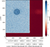 |
Fig. 1 Exposure o4wt03020 taken on 14 September 1998. Uranus in Lyα is seen as a dark blue blob and the black circle represents 1 RU . See Sect. 2.1, first paragraph for the meanings of nominal and offset wavelength axes. |
2.1 Data processing and Lyα image extraction
In the 1998 observation set-up, Uranus was positioned with an offset of 3″ along x-axis and 2″ along y-axis to the nominal target pointing. The x-axis offset was done to move the Uranus Lyα signal away from the short-wavelength cut-off of the grating spectrum and y-axis offset was done to move Uranus away from the shadow of STIS FUV MAMA detector’s repeller wire3. For 2011 observations, the offsets of 1″ and 2″ were used along the x and y axes, respectively. In Fig. 1, we show the nominal as well as the offset wavelength axes. Even though the target position on the detector is specified in the observations set-up, there is a small uncertainty in the actual position of the target and therefore the position of Uranus’ disk needed to be determined from the data itself. We explain our procedure to determine the disk position in Appendix A.
Figure 2 sketches the sources of Lyα signal in the exposures. These are emissions from H and H2 from Uranus’ upper atmosphere, emissions from background and foreground IPH, and geocorona. While the IPH signal can be assumed to be constant over a particular observation day and the line of sight (LOS), the geocorona signal varies rapidly as HST moves in its orbit around the Earth. This is because HST is well inside the Earth’s hydrogen exosphere and the sunlit part of the exosphere scatters a higher amount of Lyα signal compared to the darker part and there is a variation in the H density of dayside and nightside part of the Earth’s exosphere (e.g. Baliukin et al. 2019). Since we are interested in the signal from Uranus, a desirable observation would be the one containing minimal contamination from the geocorona (noting that the contribution from IPH signal is unavoidable). The 1998 and 2011 campaigns had four and two HST orbits, respectively, dedicated for 25MAMA-G140L aperture-grating configuration. In each of these orbits, two exposures of Uranus were taken with a total of eight (1998) and four (2011) exposures. Out of the two exposures per orbit, one exposure contained large and the other comparatively lower contamination by the geocorona. To maximise the signal-to-noise ratio (S/N) of Uranus’ signal, we only considered the exposures with lower contamination by the geocorona; thus, a total of four exposures from the 1998 campaign and two from the 2011 campaign. Table 1 lists details of these high S/N observations.
To estimate the signal from the planet, we first determined an average sky Lyα brightness (i.e. of IPH emissions and geocorona) in regions far from Uranus’ disk in the images. We then subtracted this constant brightness from the entire image. In images from both the observation campaigns, the average on- disk S/N in one pixel after subtracting sky Lyα contributions is ~1. For the further processing, we converted the pixel intensities from counts to Rayleigh (1 R = 106/4π photons/cm2 /s/sr), a widely adopted unit for airglow and aurora. For the conversion, we used the Lyα line centre throughput value of the G140L grating. Our estimated sky Lyα brightnesses for the exposures (given in Table 1) were 2580, 2565, 2490, 2465, 3070, and 3105 R, respectively. Panels A and B in Fig. 3 show the sky Lyα brightness subtracted, averaged high S/N exposures from 1998 and 2011 observations, respectively. These images show area up to 2 RU and are smoothed using Gaussian filter with σ = 5 for the display purposes only. These are the first instantaneous Lyα images of Uranus obtained in their entirety (Voyager 2 images were created by combining several images from the narrow slit). We find that the only important brightness variations are in the radial direction from disk centre (i.e, there is no significant azimuthal brightness variation). This is expected for low phase angle observations and also due to a small (~2 pixels) difference between the equatorial and polar radius of Uranus. Thus, we assume Uranus’ brightness in the images to be radially symmetric. Due to relatively low S/N in the original images, binning of pixel intensities is required to increase the S/N and, hence, to reduce the statistical uncertainty. Thus, taking advantage of negligible azimuthal variation in the brightness, we calculated the radial brightness profiles from the images.
 |
Fig. 2 Lyα emission sources in HST exposures of Uranus. The light green shade represents IPH. We note that the foreground means the part of the line of sight path that is in between Uranus and Earth, and background means behind Uranus. The figure is not to scale. |
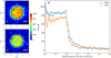 |
Fig. 3 HST observations of Uranus’ Lyα emissions used in this study. Panels A and B: high S/N exposures average images (in native HST detector frame and smoothed for display purposes only). S denotes the position of Uranus’ geometric south pole in all 1998 exposures, while N represents that of north pole in the exposure taken on 31 August 2021. Finally, 0 RU represents the centre of Uranus in the STIS images. Panel C: average radial Lyα profiles. |
2.2 Radial brightness profiles
To create the radial brightness profiles, we considered annular bins, with a centre set at the centre of Uranus. The bins have inner and outer boundaries as [R, R+dR), where R and dR are the absolute distance from the centre of Uranus and the width of the bin, respectively, in pixels. We considered dR = 5 pixels. The average intensity of pixels in the annular bin represents the intensity of that bin and the [R, R+dR) pixels of the radial profile. We could generate the radial profiles up to 300 radial pixels or ~4 RU in the 1998 and 2011 images. We considered the error array associated with the data array (image) as initial uncertainties, and they were propagated using Gaussian error propagation. Uncertainties decrease monotonically as we go further in the radial direction due to a monotonic increase in the number of pixels in the bins. The radial brightness profiles for 1998 and 2011 images are shown in Panel C of Fig. 3. These are the average profiles of the high S/N exposures of the respective campaigns, and the shaded portion in the profiles indicate the uncertainties. We note that both profiles show non-zero brightness values at distances as far as 4 RU, revealing the highly extended exosphere of Uranus. The exobase at ~6500 km altitude (see Sect. 3.1) is located at ~1.25 RU in the radial direction. Moreover, the 2011 profile shows lower intensities from 0 to ~1.75 RU as compared to the 1998 profile. From 1.75 to 4 RU the differences are smaller than the statistical uncertainties.
We subtracted the constant values of sky Lyα brightnesses from the STIS images before creating radial profiles. But since some of the sky Lyα signal originates from the IPH behind Uranus, this fraction would be completely and partially blocked by the planet and its atmosphere, respectively. This leads to over-subtraction of Lyα signal from Uranus, and we need to correct for it. For this correction we estimated the IPH Lyα brightness from Uranus to infinity along the LOS (BG IPH Lyα brightness) using the model described in Pryor et al. (2013, 2022, 2024) (Pryor IPH Model), and our brightness values are 138 and 136 R, respectively, for the 1998 and 2011 observations. Uranus’ disk completely blocks this BG IPH emissions, and thus we need to add back 100% of the BG IPH brightness to the on-disk part of Uranus’ radial profiles obtained from the STIS images. The radial brightness profiles shown in Fig. 3 have been corrected for this, where the on-disk part of the profile spans from 0 to 1 RU. The correction for the off-disk part of the profile depends on the atmospheric properties (number densities of constituents, temperature, etc.) and with varying assumed atmosphere, the correction should vary. Thus, instead of correcting the brightness profiles from the data, we did the correction to the model brightness profiles, and this procedure is explained in Sect. 3.3. The last column in Table 1 lists the disk brightnesses (corrected for the BG IPH brightness) for the analysed individual exposures. For 1998, the minimum and maximum disk brightnesses in the exposures were 838 ± 12 and 886 ± 12 R, respectively; while for 2011, they were 701 ± 12 and 750 ± 12 R, respectively. Here, the ±12 represents the uncertainty. The Uranian disk in the STIS images consisted of 17 645 pixels, thus resulting to such a low uncertainty for the disk brightnesses.
As discussed in Sect. 1, a Raman feature of 40 ± 20 R at 1280 Å was observed at Uranus through Voyager 2 measurements. From Fig. 1, we see that the region containing the Lyα signal also ranges to 1280 Å (see x-axis). The Raman signal would be confined to the disk of Uranus centred at 1280 Å (i.e. of radius of 75 pixels in the images) and is located ~112 pixels right in the x direction with respect to the Lyα disk shown by the black circle in Fig. 1. We could not identify a systematically increased brightness from the disk at the Raman feature (1280 Å), likely due to the low intensity of 20 R (when considering Voyager 2 UVS re-calibration proposed by Quémerais et al. 2013) compared to the bright Lyα signal of several hundred Rayleigh. Since our radial bins cover a significant area of the image where Raman signal is absent and due to its low brightness, we neglected any extra processing to remove the Raman signal.
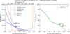 |
Fig. 4 Voyager 2 and extended Moses et al. (2018) atmospheric profiles (T∞ = 800 K for Bates extension) of Uranus. |


3 Modelling
3.1 Lyα radiative transfer in Uranus’ atmosphere
In Uranus’ atmosphere, Lyα radiation is altered primarily by resonant scattering by H, Rayleigh scattering by H2, and absorption by hydrocarbons, mostly methane (CH4). For Lyα radiative transfer in Uranus’ atmosphere, we used an adapted REDISTER code (Gladstone 1982), used in similar studies for other Solar System planets, for example, Earth and Jupiter (Gladstone 1988; Gladstone et al. 2004). The model considers a 1D planeparallel atmosphere, and we ran it for multiple solar zenith angles, thereby taking the sphericity of the atmosphere into account. Inside the atmosphere, scattering of photons is solved using Feautrier’s method. For each solar zenith angle run, the after-scattering source functions and extinctions are calculated for each atmospheric level. The after-scattering source functions and extinctions (from multiple solar zenith angle runs) are then interpolated along the LOS to calculate the emergent radiation from Uranus’ atmosphere by formal solution of the radiative transfer equation. The observation phase angle was taken into account to calculate the emergent radiation.
Our atmospheric profiles are described by ambient temperature and number densities of ambient H, H2, and CH4 (we neglect He since it is not relevant for Lyα radiative transfer) with 200 atmospheric layers until 7 RU above 1 bar level. In addition to the profile of ambient H, which has the same temperature as other species in the atmosphere (ambient temperature), we consider a population of hot H described by a separate profile for temperature and number density which falls off slowly compared to ambient H. Figure 4 shows the base atmospheric profiles used in our study. One is determined through Voyager 2 observations and another is described by Moses et al. (2018), considering multiple observations and photochemical modelling (hereafter, the ‘Moses’ profile). For the Voyager 2 profile, ambient T and number densities of ambient H, H2, and hydrocarbons up to the exobase (~6500 km) are as shown in Fig. 16 from Herbert et al. (1987), and the number densities of the ambient H above the exobase and the hot H are as shown in Fig. 2 from Herbert & Hall (1996). We assumed 2 eV for the temperature of the hot H population, as suggested in their study, for our base Voyager 2 profile. The original Moses profile (which is up to 2800 km) is extended until the exobase using the atmosphere extension formalism by Bates (1959), with T∞ = 800 K. From the exobase until 7 RU, we calculated the exospheric densities using the exosphere model described by Aamodt & Case (1962). In the following, we refer to this model as the ‘extended Moses’ model.
Since Moses et al. (2018) did not consider a hot H profile, we used the Voyager 2 hot H profile for the Moses atmosphere profile as well. We modelled the atmosphere until a large radial distance of 7 RU due to the extendedness of Uranus’ atmosphere, and the simulation boundary was chosen such that the Lyα line centre optical depth is negligible at this outer boundary. The density of hot H surpasses the density of ambient H at altitudes of ~24 000 and 15 000 km, respectively, for Voyager-2 and Moses atmospheres. At the simulation boundary, with hot H as the only constituent with a number density of ~30/cm3, considering a temperature of 2 eV, the atmospheric pressure is 0.1 femtobar.
For resonant scattering by H, we considered Voigt profile for the cross-section and our value for Lyα line centre cross-section is 4.17 × 10⁻¹³ cm2 at the reference temperature of 200 K. We then scaled the cross-section profile to the temperature of the modelled atmospheric layer. For Rayleigh scattering and absorption by methane we considered cross-sections at the Lyα line centre only, and we used constant values 2.13 × 10⁻²⁴ cm2 (Ford & Browne 1973) and 1.9 × 10⁻¹⁷ cm2 (Vatsa & Volpp 2001), respectively, which were determined at temperature of 300 K. We did not calculate the Rayleigh-Raman scattering of Lyα by H2 in this study.
For the external radiation source, we considered solar Lyα radiation. We obtained the composite Solar Lyα fluxes at 1 AU from the LISIRD4 database with adjusted solar longitudes of Earth and Uranus, and scaled them with the Sun-Uranus distances. For 1998 and 2011 observations, the solar Lyα photon fluxes at Uranus were 1.17 × 10⁹ and 1.10 × 10⁹ photons/cm2/s, respectively. We modelled solar Lyα line profile by summing two equal and opposite Gaussians with two equal and offset Lorentzians, as described by Gladstone et al. (2015). At Uranus (~20 AU from the Sun), the Lyα brightness of and illumination by the IPH as compared to solar illumination is non-negligible. In Appendix B, we explain our detailed analysis of the IPH as a potential additional external source of Lyα at Uranus and our reasoning to consider only solar illumination as a Lyα source.
The final output of radiative transfer runs that we used in our analysis is a hyperspectral image or spectral cube, in which each 2D spatial pixel contains Lyα line emanating from Uranus’ atmosphere. This is necessary because looking towards the planet the shape of emanating Lyα line from Uranus’ atmosphere varies radially, that is, from the disk centre towards the atmosphere boundary; and along with the Doppler shift, the line shape can directly dictate how much of the original signal is transmitted (or attenuated) through the foreground IPH (FG IPH) and EEH.
3.2 Extinction of Uranus’ Lyα signal by foreground IPH and EEH
The Solar System is passing through a local interstellar medium primarily composed of atomic hydrogen and helium. The heliosphere is populated by neutral H and He atoms primarily sourced from the interstellar cloud, and this population is collectively called interplanetary medium. The IPH has been investigated since the start of space-based observations, primarily through investigation of sky Lyα emissions from H (see e.g. Baliukin et al. 2022, Gladstone et al. 2018 and references therein). The IPH properties determined through numerous studies show a range of values (Izmodenov 2009; Baliukin et al. 2022). We adopted following values: temperature, TIPH = 15 000 K (e.g. Izmodenov et al. 2013), flow velocity, vIPH = 20 km/s (e.g. Quémerais et al. 2009) and downstream direction in ecliptic longitude and latitude, (λ,β) = (72.5°, –8.9°; e.g. Lallement et al. 2010). These values are similar to those adopted by Gladstone et al. 2018. Assuming a Maxwellian distribution for IPH atoms, we calculated the IPH Lyα scattering cross-section as (Chamberlain & Hunten 1987)
 (1)
(1)
where e and me are the charge and mass of the electron, respectively, c is the speed of light, fLyα is the oscillator strength at Lyα (fLyα = 0.416), λ0 is the Lyα wavelength, and Φλ is the Doppler profile for a Maxwellian distribution.
Numerous studies such as Thomas (1978) and Wu & Judge (1979) showed that the number density of IPH varies with respect to the distance from the Sun, r, and the angle, θ, measured from the upwind direction of the IPH flow. Figure 5 shows the observation geometries for the two HST campaigns. During 1998 and 2011 HST observations (r, θ) were (19.87 AU, 60°) and (20.08 AU, 110°), respectively. Thomas (1978) provided tabulated IPH number density profiles up to 100 AU for several different θ, including θ = 60 ° and 120 °. They calculated the number density profiles from their ‘hot’ model for IPH number density and used n∞, asymptotic interstellar hydrogen density of 1 /cm3. Since this n∞ is a coefficient in the hot model’s expression, the IPH number density profile can be scaled by any n∞ value. Recently, Swaczyna et al. (2020) determined the IPH number density at the heliosphere’s termination shock to be 0.127/cm3. Thus, in our analysis of 1998 and 2011 HST observations, we used Thomas (1978) IPH number density profiles for θ = 60° and 120°, respectively scaled by n∞ = 0.127/cm3. During the 1998 and 2011 HST observations, the distance between HST and Uranus was ~ 19.12 and 19.16 AU; thus, we calculated a Lyα line centre optical depth (τ) of ~1.05 and 0.78, respectively, for the foreground IPH (Fig. 2). During 1998 and 2011 observations, with respect to the foreground IPH (FG IPH), Uranus had LOS relative velocity of 10.75 km/s away from and 7.01 km/s towards the FG IPH, respectively. Thus, along the LOS, Uranus’ signal was red- and blueshifted, respectively, in FG IPH’s frame. This variation in Doppler shift leads to variation in extinction of Uranus’ signal by the FG IPH.
After passing through the FG IPH, Uranus’ Lyα signal encounters the Earth’s exosphere before getting detected by HST. The H atoms in the Earth’s exosphere (EEH), which are also responsible for the geocorona, are produced by photodissociation of water and methane in the middle atmosphere of the Earth (at altitudes below 100 km) and, according to the recent study by Baliukin et al. (2019), the geocorona extends beyond the Moon (~60 Earth radii). They retrieved the EEH number density using Solar Wind Anisotropies/Solar and Heliospheric Observatory (SWAN/SOHO) observations. Their number density profile gives us a reference, which we can use to calculate EEH column density along the LOS, needed to estimate the extinction of Uranus’ signal by EEH. However, Baliukin et al. (2019) assumed a radially symmetric profile to retrieve the radial number density profile from SWAN/SOHO observations, but it has been observed that EEH number density varies from day-side to the night-side of the Earth (and thus along the HST LOS). The atmospheric model NRLMSIS 2.05 (Emmert et al. 2021) gives the number densities and temperature of atomic H (and other neutral species) in Earth’s atmosphere up to 1000 km and takes into account the time and spatial variability. Thus, to calculate the LOS EEH column density during HST observations, we combined inputs from NRLMSIS 2.0 model and Baliukin et al. (2019) EEH number density profile. We estimated the average LOS EEH column density for 1998 and 2011 observations as 2.6 × 10¹³ and 2.9 × 1013 cm–2, respectively. We assumed a constant EEH temperature of 1000 K and calculated Lyα scattering cross-section in a same way as that for FG IPH. The average LOS radial velocity of Uranus with respect to Earth (and thus the EEH) was 20.3 km/s away from the Earth and 12.1 km/s towards the Earth for 1998 and 2011 observations, respectively. In the EEH rest frame, the Uranus’ signal is red- and blue-shifted in 1998 and 2011, respectively. We assumed the Doppler shift from the rotational motion of Uranus’ atmosphere (maximum ~2.6 km/s) is negligible.
As described in Sect. 3.1, we used the spectral image as a final output from the radiative transfer run for a particular atmospheric profile and input parameters. We then calculated the extinction of this spectral image by FG IPH and EEH accounting for the two Doppler shifts. Finally, we line-integrated the attenuated spectral image, adjusted the spatial resolution to the data, and smeared it using the STIS FUV MAMA detector’s point spread function for the Lyα wavelength. This simulates the image that the detector would record for Uranus’ observations (except the photon noise). Then we applied the same processing as we applied to the data to create radial brightness profiles. We then compared the brightness profiles from data and model to find atmospheric profiles that yield good agreement.
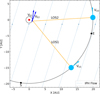 |
Fig. 5 Observation geometries for 1998 and 2011 observations. Red, dark blue, and sky blue disks represent Sun, Earth, and Uranus, respectively. Here, VE1 and VE2 represent the orbital velocity direction of Earth during 1998 and 2011 observations, respectively, and VU1 and VU2 represent the same for Uranus. Vector sizes do not represent their magnitudes, and the Sun and planet sizes are not to scale. LOS1 and LOS2 denote the lines of sight during 1998 and 2011 observations, respectively. IPH flow direction is considered to be constant during both the observation campaigns. Locations S and E in Uranus’ orbit represent southern summer solstice (1986) and northern spring equinox (2007), respectively, at Uranus. |
3.3 Transmission of background IPH Lyα signal through Uranus’ atmosphere
As described in Sect. 2.2, the calculated BG IPH brightnesses during 1998 and 2011 STIS observations were 138 and 136 R, respectively. Based on the reasoning given in Sect. 2.2, we added back 100% of these values to the on-disk part of the radial profiles derived from the STIS observations. In this section, we describe our correction procedure for the off-disk part of the radial profiles.
The ambient and hot H in Uranus’ atmosphere attenuates some of the LOS BG IPH Lyα signal, while the LOS attenuation by Rayleigh scattering due to H2 is negligible. For the 1998 and 2011 observations, along the LOS, Uranus had relative velocities of 10.75 km/s towards and 7.01 km/s away from the BG IPH, respectively. This led to a blue and red shift in the BG IPH signal with respect to H in Uranus’ atmosphere. We considered a Gaussian line profile for the BG IPH Lyα emissions with the same temperature as that of the FG IPH (15 000 K) and calculated their LOS transmissions through Uranus’ atmosphere by accounting for these Doppler shifts. The varying number densities and temperatures of ambient and hot H along the LOS leads to varying optical depth and thus transmission of the BG IPH signal. This leads to a LOS transmission profile with a gradual increase in transmission (or decrease in attenuation) of BG IPH signal from Uranus’ limb to the outer edge of the atmosphere. Instead of correcting the radial profile from the data, we corrected Uranus’ modelled radial profile. Thus, for the correction, we subtracted the line-integrated attenuation profile (complementary of the transmission profile) of BG IPH signal from the off-disk pixels of Uranus’ modelled radial profiles in order to correct for the oversubtraction in the data processing. We note that we did the correction ‘after’ we calculated Uranus’ modelled radial profile, considering the attenuation by FG IPH and EEH. An example of this procedure is shown in Sect. 4.2.
4 Results and discussion
4.1 Comparison of HST Lyα brightness with IUE and Voyager 2 results
The average Lyα on-disk brightnesses in HST observations from 1998 and 2011 are 860 ± 6 R and 725 ± 9 R, respectively. The average brightness deduced by Clarke et al. (1986) from the IUE observations was 1400 ± 450 R, thus significantly higher. They used an area with diameter of 9″ centred at the peak of Uranus’ emissions in the IUE exposures as a total signal from Uranus. When we summed the brightness over an area with diameter of 9″ centred on Uranus’ disk in the STIS images and divided by the actual disk size of Uranus (with the diameter of 3.69″), we obtained brightnesses of 1400 ± 25 and 1140 ± 25 R from the 1998 and 2011 exposures, respectively. These brightnesses are within the uncertainty margins of the IUE-derived average brightness. However, the minimum (790 ± 250 R) and maximum (2590 ± 300 R) brightnesses of Uranus derived from the IUE exceed the 450 R standard deviation of the average brightness. Table 1 lists Uranus’ disk brightnesses derived from the individual HST exposures. The variability in IUE brightnesses with time or exposures far exceeds that of the disk brightnesses in HST exposures. Since the IUE telescope was designed to record spectrum, the spatial distribution of the brightness in Uranus’ observations was not available. Also, IUE observations have substantially lower spectral resolution than STIS ones. Thus, when uncertainties are taken into account, although some of the difference between IUE and STIS brightnesses might be due to the changes in Uranus’ atmosphere or auroral activity, we cannot exclude that a large part of it (or even all) might come from the instrument, calibration, and processing differences. While it is evident that STIS observations have lower uncertainties than IUE, we do not go further into the details of this comparison.
During the Voyager 2 flyby, the first spatially resolved Lyα brightness profile of Uranus was obtained. Figure 6 in Strobel et al. (1991) shows Uranus’ Lyα brightness profile obtained by Voyager 2 at an observation phase angle of 43°. The profile shows average on-disk brightness of ~1500 R. Quémerais et al. (2013) proposed re-calibration for the Voyager 2 UVS instrument from the IPH observations, and it was corroborated by recent study on Saturn by Koskinen et al. (2020). The general suggestion from this recalibration is to reduce the Lyα intensities deduced from Voyager 2 UVS observations approximately by a factor of 2. Considering this, Uranus’ average on-disk Lyα brightness from Voyager 2 observations results to ~750 R and thus closer to the HST observed brightnesses (note that Voyager 2 observations were not affected by FG IPH and EEH as they were taken during a close flyby of the planet). There is a strong intensity variation and asymmetry near the limb in the Voyager 2 radial brightness profile, which is expected for high phase angle observations. Since HST observations were taken at low phase angles (≤2°) the intensity variation near the limb is comparatively lower and hardly detectable in the STIS images. Moreover, the pixel binning to create the radial brightness profiles would further wash out any intensity variation near the limb, making the on-disk HST radial brightness profile rather flat.
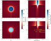 |
Fig. 6 Results from radiative transfer modelling for Voyager 2 base atmosphere and 1998 observing conditions. Left column: modelled original (above) and attenuated by FG IPH and EEH (below) Lyα line-integrated intensities from Uranus’ atmosphere. Right column: line-resolved intensities for the radial pixels from the respective images in the left column. The Lyα lines are represented in Earth’s frame. All Doppler shifts are properly accounted for calculating the attenuation. |
4.2 Comparison of observed and modelled Lyα brightness profiles
We started our analysis with Uranus’ Voyager 2 base atmospheric profile. Figure 6 shows model results for 1998 observing conditions. The left column shows Uranus’ original and attenuated (by FG IPH and EEH) Lyα line-integrated brightnesses. The right column shows line-resolved original and attenuated spectral brightnesses for the pixels from the middle half row/column in the images, where the first pixel is the central pixel on the disk and the last pixel is at the lower end of the image (shown as a solid yellow line). In the upper right panel, we see how the Lyα line shape in the original spectral image changes with distance from the disk centre. Due to the varying line shape, the attenuation across the line by the FG IPH and EEH (lower right panel) is also changing. For the 1998 observations, the extinction by the FG IPH is strongest in the central part of the Doppler shifted lines of Uranus’ spectral image, while the extinction from EEH occurs in the blue wing of the lines that are wide enough to stretch up to EEH extinction band when they arrive at the Earth. We note that for 1998 conditions, the Doppler shift of Uranus’ signal with respect to the EEH is larger compared to the FG IPH.
The left panel in the Fig. 7 shows our correction procedure for the transmission of the BG IPH signal by Uranus’ atmosphere (Sect. 3.3). We show the example for Voyager 2 base atmosphere model with 1998 observing conditions. For the correction, we subtracted the LOS attenuation brightness profile of BG IPH from Uranus’ attenuated radial brightness profile. All the modelled radial brightness profiles shown in this work are corrected for BG IPH transmission for the respective atmospheric model profile.
The right panel in Fig. 7 shows the radial brightness profiles from data and model for 1998 and 2011 observing conditions. Here we use the same atmospheric profile for the particular model (Voyager 2 or extended Moses) but input solar fluxes, observation phase angles, and extinctions by FG IPH and EEH are adjusted to the 1998 and 2011 conditions (values mentioned in the previous sections). For both the years, the modelled brightness profiles have consistently lower values than the observed ones up to ~2.5 RU. For the 1998 observations, the observed and modelled profiles show agreement from ~2.5 RU onward while for 2011, the agreement starts from ~3.3 RU onward (not shown in the figure). It is coincidental that the modelled brightness profiles for a particular atmospheric model look almost identical for 1998 and 2011 observing conditions. The average on-disk brightness obtained from the extended Moses profile is substantially lower than that from the Voyager 2 model.
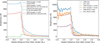 |
Fig. 7 Comparison of observed and modelled radial brightness profiles. Left: Our procedure to correct the modelled Uranus brightness profile for the transmission of BG IPH, with the example of Voyager 2 model and 1998 observing conditions. Right: 1998 and 2011 data average radial Lyα profiles compared with modelled radial profiles with Voyager 2 and Moses atmospheric profiles. For the two HST observations, the average on-disk brightnesses are 860 ± 6 and 725 ± 9 R, respectively. We note that all the modelled profiles are corrected for the BG IPH transmission. |
4.3 Adjusting the model atmosphere
4.3.1 Initial considerations and tests
For the on-disk intensity of Uranus’ Lyα emissions, scattering in all atmospheric layers contributes to the signal, while the off-disk signal is from scattering primarily in the upper atmosphere only. Since the exosphere is mainly composed of atomic hydrogen, the parameters that primarily influence the brightness are the number densities and temperatures of the hot H in the extended exosphere, followed by those of ambient H. While for the on-disk intensity, the additional parameters that influence the brightness are the ambient temperature in the lower atmosphere (below exobase) and the number densities and profiles of H2 and CH4 . We first adjusted the parameters of atomic hydrogen for a better agreement of data and model off the disk, then we changed the parameters of the bulk atmosphere, which affects the on-disk signal only.
To increase the off-disk brightness, we preferred not to modify the number density or temperature of ambient (thermospheric) H, because to obtain the brightnesses we observe in the data, we require a substantial amount of ambient H at altitudes well above the exobase in the model atmosphere, which seems unrealistic. On the other hand, since hot H scatters the incident solar Lyα radiation more efficiently, it is required in smaller quantities than ambient H. Thus, we first attempted to modify the hot H profile deduced from Voyager 2 observations, which extends to higher altitudes (Herbert & Hall 1996). The hot H number density profile proposed by them is ∝ 1/r2, where r is the planetocentric distance, and they suggested temperature of hot H population to be ~2 eV. From Fig. 7, we see that 2.5 RU onward, the hot H profile from Voyager 2 delivers the appropriate data-model brightness agreement, however, it does not explain the brightness between 1 and 2.5 RU. We found that increasing the temperature of hot H up to 20 eV (arbitrarily decided), while keeping the number density profile same showed meagre improvement in the radial brightness. On the other hand, scaling up hot H number density did increase the radial brightness, but the agreement throughout the off-disk data profile was never met. We achieved a better off-disk brightness agreement with a hot H profile falling off more rapidly than 1/r2 and with scaled up initial number density. We retained the Voyager 2 hot H profile, which matches the data at >2.5 RU, without modifying it, and we propose that another, steeper hot H profile is needed, in particular, to explain the brightness between 1 and ~2.5 RU.
In the atmospheres of giant planets, hot H can be produced in multiple pathways such as photoionisation and photodissociation of H2 , and through energetic particle precipitation, as discussed by Bisikalo et al. (1996) for Jupiter. These primary processes, along with secondary processes, produce hot H having a wide range of temperatures, making it evident that multiple populations/profiles of hot H should co-exist in giant planets’ atmospheres. Thus, to achieve a better model-data radial brightness agreement, we introduce another profile of hot H along with the unmodified Voyager 2 hot H profile. Hereafter, we denote this new population of hot H as H* and the Voyager 2 population representing escaping hot H as  . To set up an appropriate profile for H*, we considered possible generation mechanisms at Uranus first. Although multiple hot H profiles in Uranus’ atmosphere can exist, we modelled with only one more profile for simplicity. Thus, through this profile, we attempted to model the bulk of possibly non-escaping hot H population.
4.3.2 The H* model profile
Although auroral energetic particle precipitation can occur across the lower latitudes due to magnetic field orientation of Uranus, the aurorae observed so far are rather weak and transient as compared to Jupiter or Saturn (Bhardwaj & Gladstone 2000; Lamy et al. 2017). Furthermore, the properties of the auroral particles are not well understood so far. Thus, we did not consider auroral precipitation for the generation of the global hot hydrogen population. The derived hot hydrogen abundance might be generated from photochemical reactions. In giant planets’ atmospheres H2 undergoes the following photochemical reactions due to solar soft X-ray and EUV photons (e.g. Huebner & Mukherjee 2015):
 (2a)
(2a)
 (2b)
(2b)
 (2c)
(2c)
 (2d)
(2d)
where hν represents a photon, Hhot a hot hydrogen atom, and H(2s, 2p) an excited hydrogen atom. Among these four reactions, reaction 2a primarily produces hot H, for photons in the spectral range of 930 to 1110 Å (with H2 photo ionisation and dissociation cross-sections from the PHIDRATES6 database). Considering the enthalpy of formation of one H atom to be 2.26 eV (Schunk & Nagy 2009), this reaction produces hot H with energies in the range of ~3.3 to 4.4 eV. The  formed in reaction 2c reacts very quickly with H2 to form
  (see, e.g. Melin 2020) which in turn can undergo dissociative recombination with electrons. All of these reactions can produce hot H in the following ways:
 (3a)
(3a)
 (3b)
(3b)
 (3c)
(3c)
Assuming that the reactants and products are in respective ground states, the hot H atoms formed in reactions 3a to 3c have energies of 1.28, 6.15, and 1.59 eV, respectively (Erik Vigren, private communication). The hot H formed in all of the above reactions can be approximated by a Chapman-like profile. Our analysis with Voyager 2 H2 profile shows that the peak productions for photo products in reactions 2a to 2d occur in the altitude range of ~1000 to 3000 km. The calculations were done for multiple solar zenith angles. Since  peaks at the similar altitude range (Moore et al. 2019), we assumed that hot H produced in reactions 3a to 3c also peak in the range of ~1000 to 3000 km. Our H* number density profile resembles that of generalised Chapman profile for ion production, given by
 (4)
(4)
where nmax is the peak H density at the altitude 𝓏max, ξ = 𝓏 – 𝓏max, where 𝓏 is the altitude, and H is the scale height. We assumed H* column density N, as a free parameter. Our remaining free parameters are 𝓏max, and H or the H* temperature, T. For relating H and T via H = kBT/m𝑔, we considered the 𝑔 value at the exobase (𝑔Uranus–exobase = 5.64 m/s2). For a particular set of these parameter values, nmax was then obtained by integrating Eq. (4) over altitudes and then inverting it, since the left-hand side is the column density of the H* profile. To summarise, our H* profile is described by the parameters set  . We note that in Eq. (4), we neglected the term for solar zenith angle present in the generalised Chapman profile for ion production, but the effect of varying solar zenith angle is indirectly addressed when we analyse the effect of varying 𝓏max . Also, we did not take into account the destruction and transport mechanisms of H* in our empirical analysis. While this is clearly a simplification, addressing these aspects is beyond the scope of this paper.
We carried out a simplified collision analysis in which we considered hard-sphere collisions of hot H with ambient H and H2 only, since they are the dominant components of the upper atmosphere. This collision analysis shows that hot H atoms produced below ~4000 km undergo substantial collisions. Since reactions 2 and 3 produce hot H with different energies at a range of altitudes, which further undergo collisions below exobase, hot H populations with various energies should exist in Uranus’ atmosphere. However, consideration of variable hot H temperature due to collisions makes radiative transfer calculations tedious, especially when we do not use a Monte Carlo code. Thus, in our analysis, for a particular radiative transfer run, we considered a single temperature for an H* profile. We find that various H* profiles with the base Voyager 2 atmospheric model yield good agreement for the data-model off-disk brightness. For 1998, H* profiles with H/T range of 2500 km/0.15 eV to 6000 km/0.35 eV give good fits. While for 2011, H* profiles with H/ T range of 3000 km/0.17 eV to 35 000 km/2 eV give good fits. We find that the brightness profile sensitivity for 𝓏max in the range of 1000 to 3000 km is negligible, and we considered 𝓏max = 3000 km only in our further calculations.
For simplicity and direct qualitative comparison of the required H* abundance, we considered H* profiles with the same temperature and corresponding scale height of 0.3 eV and 5000 km. The profiles with these parameters yield good fits to the data-model brightness profiles for both years. The dashed green and solid red profiles in the left panel in Fig. 8 show the model brightness profiles for 1998 and 2011 observations, respectively, obtained by introducing H* population to the base Voyager 2 atmospheric model. The Chapman profile parameters, (T, 𝓏max, H, N) for 1998 and 2011 reference H* populations are (0.3 eV, 3000 km, 5000 km, 0.075% of Voyager 2 base ambient H) and (0.3 eV, 3000 km, 5000 km, 0.05% of Voyager 2 base ambient H), respectively. The Voyager 2 escaping hot H  profile (temperature of 2 eV) is unchanged. The Voyager 2 base ambient H column density in our model is ~2.8 × 1017 cm−2. Thus, the column densities of the reference bound hot H populations are 2.1 × 10¹⁴ and 1.4 × 1014 cm−2 for 1998 and 2011, respectively. The column density of the escaping
  and thus more than an order of magnitude lower than these reference bound H* abundances derived here. The H* profile is steeper than
  profile (right panel in Fig. 8) and dominates the Lyα scattering in the region of ~1 to 2.5 RU in the radial brightness profile. A slight disagreement of the 1998 data – reference model brightness profiles in the region ~1.6 to 2.3 RU might indicate the need for the addition of another, hotter H* population along with the relatively colder reference H* population.
4.3.3 Adjusting the ambient atmosphere
For 2011, we already obtained good agreement in the entire observed brightness profile with the addition of the H* population to the Voyager 2 base model, and thus no changes to the ambient atmosphere are needed. However, for 1998, the model on-disk brightness (dashed green line in the left panel in Fig. 8) is lower than the observed one, demanding adjustments to the ambient atmosphere. We adjusted the density of the ambient atmosphere, retaining the same profile shapes from the Voyager 2 base profiles. We scaled the profiles of H, H2 , or CH4 individually by a constant number. The scaling factor required for ambient H number density profile is the smallest, followed by that for H2 and CH4. Upscaling the density of H or H2 and downscaling the CH4 produces brightness profiles that agree similarly well with the data in the on-disk region. Here, we propose the increased abundance of ambient H (as the atmospheric constituent requiring the least modification) as the preferred solution. However, in reality, the combination of changes in these atmospheric constituents might cause the observed on-disk brightness. Thus, our solutions for number densities are degenerate. Since the Moses atmosphere profile would require larger adjustments than the Voyager 2 profile, we use Voyager 2 base profile only for our final modelling.
Our radiative transfer analysis indicates that variations in the ambient temperature profile have only a minimal effect on our modelled brightness profiles. Post-Voyager 2 observations, many studies attempted to improve the temperature profile of Uranus in various parts of the atmosphere. Recently, Uranus’ temperature profile in the lower atmosphere (up to stratosphere) was revisited using James Webb Space Telescope observations, and it has been found to be similar to one derived by Spitzer Space Telescope observations (Michael Roman, private communication). Another recent study used Earth-based stellar occultations to revise the temperature profiles in the upper stratosphere and lower thermosphere of Uranus (Saunders et al. 2023, 2024). However, since our radiative transfer simulations show insignificant dependence on variation in the ambient temperature profile (i.e. much smaller than the uncertainty in the data), we retain the Voyager 2 temperature profile for our modelling. We acknowledge that this temperature profile (and our extended Moses profile) implies a downward heat flux below the thermosphere. Stevens et al. (1993) already pointed out that the downward heat flux inferred from the Voyager 2 temperature profile is ~0.06 erg /cm2/s and is considerably more than the available energy deposited by solar radiation below 110 nm in the atmosphere of Uranus.
The solid green line in the left panel in Fig. 8 shows our 1998 reference model brightness profile, obtained by addition of H* population and upscaling Voyager 2 base ambient H profile by a factor of ~1.5. We can achieve similar radial brightness on the disk by upscaling the Voyager 2 H2 profile by a factor of ~2 or downscaling the CH4 profile by a factor of ~15, although with a slightly worse fit in the off-disk region, since ambient H2 and CH4 are dominant at altitudes lower than ambient H and thus have a lower effect on the off-disk brightness. Our reference radial brightness profiles for the 1998 and 2011 observations have reduced chi-square values of  and 1, respectively. The reference model disk centre and the brighter limb brightnesses (limb brightening is asymmetric due to non-zero observation phase angle) along the equator and before the attenuation by FG IPH and EEH for 1998 are 1210 R and 1320 R, respectively (difference of 110 R). For 2011, they are 990 and 1140 R, respectively (difference of 150 R). The limb brightening is not recognizable in STIS images; however, it is slightly visible in the model brightness profiles (more for 2011), even after the pixel binning, needed to create those profiles. Table 2 summarises the parameters of atomic hydrogen in Uranus’ atmosphere in our reference atmospheric profiles for 1998 and 2011.
For 1998, when we kept the ambient H density as in the Voyager 2 base profile (i.e. ambient H scale factor = 1) and only added the new hot H population, a denser H* profile with H = 3500 km/T = 0.2 eV and N = 0.24% of the Voyager 2 base ambient H yields a good fit. Thus, requiring ~5 times more abundance than for the 2011 reference profile with H = 5000 km/T = 0.3 eV population (for which the ambient H scale factor is 1).
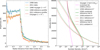 |
Fig. 8 Reference radial brightness (left) and H (right) profiles for 1998 and 2011 observations. Our 1998 and 2011 ambient atmosphere profile is identical to that of Voyager 2, except for 1998, reference ambient H profile is 1.5 × Voyager 2 base ambient H profile. For both 1998 and 2011 model atmospheres, along with Voyager 2 hot H, we introduce new hot H population (H*). The reference H* Chapman profiles shown in this figure have parameters for 1998 as |


4.3.4 H* profile parameter studies and good fit model atmospheres
We tested the sensitivity of our modelled brightness profiles to the parameters of the new hot H profile. As stated earlier, variation in the H* maximum production altitude (𝓏max) in the range of 1000–3000 km showed a negligible effect on the modelled brightness profiles, and we did not analyse zmax further. Figure 9 shows variation of modelled brightness profile with variation in the H/T (upper row) and N (bottom row) of H* profile, when varied individually. Here, when we varied H/ T (N), we kept N (H/T) and 𝓏max fixed to the reference values. We note that for fixed N and 𝓏max, with varying H/T, the distribution of hot H throughout the profile will differ. For this parametric analysis of H* profile, we varied H/T and N by 20% (we choose 20% because for 1998, we get data-model good fit  until H = 6000 km, which is 20% more than 5000 km). We find that with H/T variation, radial brightness profile shows minor and substantial variation in the on and off disk regions, respectively, of the model brightness profiles. The off-disk brightness sensitivity with H/T variation seems higher for 1998 than 2011. A 20% variation in N shows a similar or slightly higher effect in the on-disk region and a minor effect in the off-disk part of the brightness profiles compared to the variation in H/T by the same factor.
To understand what atmosphere models give reasonable fits across the entire data-model brightness profile (i.e. both, on- and off- disk), we varied H/T, N, and the ambient H scale factor simultaneously. Table 3 shows the range of these parameters that give reasonable data-model brightness fits. With a single H* population, the range of H* H/T that gives a good fit is larger for 2011 than for 1998. With a higher H* temperature or scale height, we require a lower H* abundance, since H* with higher temperature scatters Lya photons more efficiently. As H* affects the brightness more in the off-disk region than on-disk, a higher ambient H scaling is needed for hotter H*, which requires a lower abundance to obtain the off-disk brightness fit.
To determine whether solar EUV radiation is a sufficient source to supply the hot H in Uranus’ exosphere, we estimated the maximum value of the total hot H production rate through reactions 2a and 2d → 3 during the 1998 and 2011 observations, and find it to be 4.1 × 10⁸ atoms/cm2/s. For this estimation, we considered 2a to 2d reactions branch weights through PHIDRATES7 cross-sections and considered that all the solar EUV photons in the wavelength range 300 to 800 Å (for reaction 2d → 3) and 930 to 1110 Å (for reaction 2a) are absorbed. If we assume only half of them make it to the exosphere due to their random directions and collisions, and neglecting any secondary fast hot H created during collisions, during 1998 and 2011 observations, the exospheric hot H supply rate on the sunlit side from these reactions is ~2 × 10⁸ atoms/cm2/s. These hot H atoms can arrive at the exobase and launch into the exosphere in multiple directions. The time of flight for a gravitationally bound particle with a grazing circular orbit at Uranus’ exobase is ~4.2 hours, while for a particle launched radially outward into the exosphere with half the escape speed (10.65 km/s) has an exospheric lifetime of ~3.5 hours and maximum altitude of ~1.5 RU before it enters into the deeper atmosphere through exobase (Chamberlain (1963), Eqs. (114) and (115)). We considered an average lifetime of 4 hours for the gravitationally bound exospheric hot H. Assuming that the inward and outward flow of hot H in a radial column in the exosphere is in equilibrium, the column density of hot H produced from the solar source during the 1998 and 2011 observations is then ~2.9 × 1012 cm−2.
In Table 3, for both years we list the relatively colder H* populations that require substantial abundance and reduction in ambient H to obtain good fits. For 1998, the 0.15 eV population requires an abundance of 1.26 × 1015 cm−2, which is ~430 times our estimated solar source supply. This extreme abundance requirement and a large reduction required in ambient H (scaling factor of 0.45), make this population unlikely to dominate in the exosphere. Similarly, for 2011, the 0.17 eV H* population requires abundance ~290 times from the solar source supply, making it unlikely to dominate in the exosphere during 2011 observations. For 1998, the brightness fit  increases rapidly at higher H/T from H/T = 6000 km/0.35 eV population. For this profile, the required abundance is ~30 times higher than the solar origin supply. For 2011, the brightness fit is good for temperatures as high as ~1.5 eV. The
  values increase significantly for temperatures higher than ~2 eV, mainly due to data-model radial brightness profile disagreement from 2 RU onward. Since at this temperature, the most probable Maxwellian speed is comparable to the Uranus escape speed (V∞–Uranus = 21.3 km/s), at least half of the population would escape the planet (we assume that the hot H population of a particular temperature has a Maxwellian speed distribution at the exobase). Moreover, since hot H produced from solar radiation with creation temperatures between 1.28 and 6.15 eV undergoes substantial collisions below the exobase, it might cool down significantly when it reaches the exosphere. Thus, it seems unlikely that the population of this high temperature (~2 eV) dominates the gravitationally bound exosphere. Even for this 2 eV H* profile, the required abundance for good fit is still ~2.5 times the solar origin supply. Recall that we also used the escaping hot H profile determined by Herbert & Hall (1996) in our model, and this profile has an abundance of ~1.4 times the hot H supply from the solar source for 1998 and 2011. Thus, the combined hot H abundance that gives good fits to the 1998 and 2011 HST data always seems to be higher than that can be provided by the solar source, indicating that other energetic processes might significantly contribute to the hot H in Uranus’ exosphere.
From our H* profiles, it seems that Uranus has substantial hot H at higher altitudes than Jupiter (Gladstone et al. 2004) and possibly at Saturn (Tseng et al. 2013; Koskinen et al. 2020). This is possibly due to the confinement of methane (which effectively cools hot H) at lower altitudes; this, in turn, is likely due to lower Eddy diffusion at Uranus and, thus, less atmospheric mixing, compared to other giant planets (Strobel et al. 1991).
Atomic hydrogen in our reference atmosphere models for Uranus’ 1998 and 2011 HST observations.
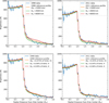 |
Fig. 9 Sensitivity of the modelled brightness profile and thus data-model brightness profile agreement to variations in H* profile scale height (H)/temperature (T) and column density (N), when varied individually. The temperatures corresponding to the H of 4000, 5000, and 6000 km are 0.23, 0.3, and 0.35 eV, respectively. |
Atmosphere profiles giving good fit to the 1998 and 2011 data brightness profiles.
5 Summary and conclusions
We examined two sets of Lyα images of Uranus taken by HST using STIS in the slit-less spectroscopy observing mode. The brightness and distribution of Lyα in the images, taken in 1998 and 2011, allow us to probe Uranus’ upper atmosphere before and after equinox at the planet in 2007. The images have a spatial resolution of ∼341 km/pixel and capture signals up to large distances of 4 RU. The images reveal a roughly constant on-disk Lyman-alpha brightness and gradually decreasing signals above the 1-bar limb, confirming the presence of a widely extended exosphere.
The average on-disk brightnesses of Uranus in 1998 and 2011 HST observations are 860 ± 6 R and 725 ± 9 R, respectively. The brightness enhancements near the planet’s limb (limb brightening) are small and not resolved in the HST data. The average on-disk brightnesses derived from HST observations are substantially lower compared to the average brightness of 1400 ± 450 R derived from the IUE observations from 1982 to 1985. However, when we took into account all emissions that are captured in the large field-of-view of IUE, we obtained brightness values of 1400 ± 25 and 1140 ± 25 R from the 1998 and 2011 STIS exposures, respectively, which are within the uncertainty of IUE-derived average brightness. The brightnesses from IUE exposures show much higher variations compared to those derived from HST exposures. Within the uncertainty margins of the average IUE brightness, the difference in IUE and HST brightnesses might be explained by difference in Uranus’ atmosphere, observing conditions, and data processing (in particular due to the lack of spatial resolution in IUE data). The Lyα brightness of 1500 R, inferred from Voyager 2 observations, is also higher than STIS derived brightnesses. However, a re-calibration of Voyager 2 UVS and consideration of the IPH effects would lead to a lower brightness, as measured from Earth, which is consistent with our HST values. While an actual change in the brightness of Uranus since the IUE and Voyager measurements in the 1980s cannot be excluded, we consider it more likely that the early values (particularly, IUE) overestimated the Lyman-alpha brightness of Uranus.
To reduce the statistical uncertainty, we worked with radial brightness profiles generated by averaging the pixel brightnesses in STIS images over annular pixel bins, starting from Uranus’ disk centre and extending as far as 4 Uranus radii (RU). The radial brightness profile for 2011 has consistently lower values until ∼1.75 RU and generally higher values between ∼1.75 and 3.3 RU than 1998 one. After ∼3.3 RU, both the brightness profiles are identical within the uncertainties.
We modelled the Lyα radiative transfer in Uranus’ atmosphere and extinction of Uranus’ Lyα signal by FG IPH and EEH. We used the REDISTER code for our radiative transfer model, and we took into account Lyα resonant scattering by H, Rayleigh scattering by H2 , and absorption by CH4 in Uranus’ atmosphere. We assessed the solar and IPH Lyα sources for 1998 and 2011 observing conditions and assumed only the solar source for the radiative transfer modelling. Since the IPH between Uranus and Earth, as well as EEH, significantly scatter Lyα radiation, it is important to take into account the extinction of Uranus’ signal by them when analysing HST data.
For 1998 and 2011 observations, the modelled brightnesses derived using Uranus’ Voyager 2 and extended Moses atmosphere profiles were lower than the brightness in the observations until 2.5 and 3.3 RU from the disk centre, respectively. The brightnesses modelled with the extended Moses atmosphere were substantially lower than those from the model assuming the Voyager 2 atmosphere.
To reproduce the observed high off-disk brightnesses, we introduced a gravitationally bound hot H exosphere, assuming a Chapman profile to the Voyager 2 atmosphere model. We find that hot H profiles with a range of temperatures/scale heights give good fit to the data, and the range of possible hot H profiles for 2011 is larger than for 1998. For some good-fit model atmospheres, in particular for 1998, slight adjustments to the Voyager 2 ambient H or H2 , or substantial adjustments to the ambient CH4 abundances (while retaining the Voyager 2 original profile shapes) are required to obtain good agreement between data and model on-disk brightnesses. Considering a same tempera- ture/scale height and maximum production altitude, the hot H exosphere profile for 2011 requires a lower abundance than the 1998 hot H exosphere profile. In such a case, the ambient H or H2 abundance required is also lower for 2011 than for 1998.
Our parametric study for sensitivity of modelled brightness profiles to the parameters of newly introduced hot H population shows that when the parameters are varied individually: a) The modelled off-disk brightnesses are more sensitive to the hot H temperature/scale height than the on-disk ones; b) Variation in the altitude of maximum production of hot H in the range of 1000 to 3000 km had negligible effects on the modelled brightnesses. Finally, we find that the hot H abundance required for our good fit profiles is greater than what can feasibly be produced by the solar EUV radiation, indicating the possible role of other energetic processes contributing significantly to the hot H in Uranus’ exosphere.
We note that this is the first reporting of this gravitationally bound hot H component. The brightness distribution in IUE data was not spatially resolvable, and this component was not detected by Herbert & Hall (1996) in Voyager 2 UVS scans either, possibly due to higher uncertainties in the aggregated scans and their assumption of radiative transport in the exosphere to be optically thin for deriving the exospheric H density profile. The dense hot H population is present in both HST datasets. Moreover, from the agreement of Uranus’ IUE and HST Lyα disk brightnesses (when the HST brightnesses were calculated in the same way as the IUE brightnesses) indicates the possible presence of dense hot H in IUE data as well. Thus, this component is likely a stable part of Uranus’ upper atmosphere. We acknowledge that our analysis of the hot H exosphere is underconstrained and it opens the observational perspectives, either from HST and/or a future in-orbit UV spectrometer, to fully constrain it.
Taken together, we present, for the first time, a consistent picture of the measurements as well as the radiative transfer modelling results, demonstrating that the Lyα emissions from Uranus can be explained by a combination of resonant and Rayleigh scattering of sunlight as the primary source. No additional excitation mechanisms, such as auroral precipitation or other sources, are needed; thus, the contributions of those are negligible. However, we find that the presence of hot H in Uranus’ exosphere cannot be explained by the solar EUV radiation alone as a source. To understand how Uranus’ upper atmosphere changes with the seasons, more observations at different epochs in Uranus’ orbit around the Sun are needed.
Acknowledgements
Sushen Joshi, Lorenz Roth, and Nickolay Ivchenko acknowledge support from the Swedish National Space Agency through PhD grant 187/20. Laurent Lamy thanks the support from the CNES space agency and CNRS/INSU national programs of heliophysics (PNST, also funded by CEA) and planetology (PNP). The authors thank Erik Vigren for discussion and calculations of energies of hot H formed in the  reactions. Finally, we thank Prof. Darrell Strobel for his review, which greatly helped to improve the manuscript. The HST/STIS data were obtained through the HST/GO programs 7439 and 12239 (PI G.E. Ballester) and are accessible with the online MAST archive at :https://archive.stsci.edu/home. They can alternately be retrieved from the online APIS service at https://apis.obspm.fr+ref https://doi.org/10.25935/T184-3B87.
Appendix A Determination of Uranus’ disk centre in STIS images
Since Uranus is a gas planet with an extended exosphere, we see a gradual transition in the Lyα intensity in the STIS images, making it challenging to accurately locate the disk. After assessing some other approaches, a comparatively reliable approach we found is as follows: initially, we chose a candidate disk centre pixel visually. We then recorded pixel intensities along multiple segments separated by uniform angular distance in the azimuthal direction and centred at the candidate centre pixel. We chose the segment lengths well enough to cover the boundaries of the disk with diameter of ~150 pixels. We then calculated χ2 value of pixel intensities for each segment pair and from those, we calculated an average χ2 for that candidate centre pixel. We repeated this process for numerous candidate centre pixels. The pixel with the minimum average χ2 then represents our Uranus’ disk centre. This is the pixel around which the intensity is most uniformly distributed. Figure A1 shows the determined disk centre with segments for exposure o4wt03020.
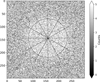 |
Fig. A1 Uranus disk centre determination for exposure o4wt03020 image. The black circle represents 1 RU. |
Appendix B Attenuation of solar Lyα line by IPH and assessment of IPH as a potential Lyα source at Uranus
Since IPH resonantly scatters Lyα photons, it is important to investigate the effects of the IPH on the solar illumination as well as IPH as a potential external Lyα source at Uranus. Modification of the solar Lyα line by the IPH varies with r and θ (see Sect. 3.2 for details of these parameters). Since direct solar radiation falls off rapidly with the distance from the Sun (1/distance2), the Lyα illumination of the planetary atmosphere by IPH, compared to the solar source, becomes important at larger distances from the Sun. It is mostly negligible at Jupiter (Roth et al. 2014; Alday et al. 2017), but non-negligible at Pluto (Gladstone et al. 2015).
We first calculated the extinction of solar line by IPH. The original and attenuated solar lines at the location of Uranus during 1998 and 2011 observations are shown in Fig. B1. It can be seen that in 1998 and 2001, 8.3% and 6.7%, respectively, of the original solar flux was attenuated by IPH. To determine IPH as a Lyα source at Uranus, we need to know the IPH brightness at the location of Uranus. For this, we used the all-sky IPH brightness map calculated by Pryor model and the maps for 1998 and 2011 observation epochs are shown in Figs. B2 and B3, respectively. It can be seen that IPH Lyα brightness varies over the sky seen from Uranus. During 1998 observations epoch, the dayside and night-side average IPH Lyα brightnesses were 402 and 158 R, while for 2011 observation epoch they were 430 and 156 R, respectively. Since the IPH flows in (roughly) one direction, when observed from a Solar System planetary body, IPH has a varying LOS velocity, and thus there is a varying Doppler shift in the IPH signal seen in different directions from Uranus. This makes the Lyα radiative transfer in Uranus’ atmosphere with IPH as a source a difficult and tedious problem to solve. Thus, we first decided to compare solar input and IPH as a Lyα source. For this analysis, we first calculated all-sky LOS IPH velocity when observed from Uranus, considering IPH downstream flow speed of 20 km/s. This all-sky LOS IPH velocity map is shown in Fig. B4. From this all-sky velocity distribution, we calculated the Doppler shifted IPH Lyα signal. We then determined the all-sky IPH Lyα radiation scatterable by Uranus’ H using an approach similar to that followed by Gladstone et al. (2015). From our radiative transfer analysis with Voyager 2 atmospheric model and solar line as input, we found that the Lyα scattering optical depth in Uranus’ atmosphere reaches to such a high extent that all the photons within ~ 2 Doppler units of the hot H (2 eV or ~23200 K), which is ~0.16 Å from the line centre, are scattered. This also implies everything within the 2 Doppler units of the ambient H with exospheric temperature of 800 K is scattered. This high amount of scattering results from confinement of hydrocarbons (esp., methane), which absorb the UV radiation, at the lower altitudes. Figure 4 shows the altitudes where the Lyα scattering and absorption optical depths ( and
and  , respectively) are unity. With the possibility of presence of hot H with temperatures > 2 eV, we expect most or all of the (Doppler shifted) IPH signal at Uranus getting scattered.
The dayside IPH Lyα photon fluxes for 1998 and 2011 observation epochs are 2 × 10⁸ and 2.14 × 10⁸ photons/cm2/s, respectively, which are 17% and 19.45% of the unattenuated solar photon fluxes of 1.17 × 10⁹ and 1.1 × 10⁹ photons/cm2/s at Uranus, for 1998 and 2011 observations, respectively. This is 8.7% and 12.75% more when compared to the attenuation of 8.3% and 6.7% of the solar fluxes for 1998 and 2011 observations. Looking at Fig. B1 it appears that, with the observation geometries of 1998 and 2011, the attenuation of solar line and the average Doppler shifted IPH Lyα illumination cover a similar spectral range. Thus, taking into account these two factors together, we estimate that the attenuation of the solar line by IPH is approximately compensated by the IPH brightness at the location of Uranus (or vice versa) and that their difference is small enough to ignore taking into account both of these effects while considering the input for our radiative transfer modelling. Thus, we considered only the ’unattenuated solar line’ as an input for the radiative transfer in Uranus’ atmosphere.
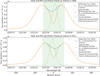 |
Fig. B1 Estimation of Lyα fluxes at Uranus during 1998 and 2011 observations. In both panels, the blue curve shows the unattenuated solar Lyα line at Uranus at the observation epochs, modelled with equal and opposite Gaussians and Lorentzians (see text), while the orange curve shows the solar Lyα line at Uranus after attenuation by IPH between the Sun and Uranus. The green shade shows dayside IPH signal band at Uranus during that epoch. The spectral limits of the bands approximately represent the maximum blue and red shifted wavelengths of dayside IPH Lyα lines. The dashed green profile represents dayside IPH summed line profile. |
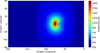 |
Fig. B2 Pryor model all-sky IPH Lyα brightness seen from Uranus at 1998 observation epoch. |
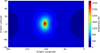 |
Fig. B3 Pryor model all-sky IPH Lyα brightness seen from Uranus at 2011 observation epoch. |
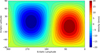 |
Fig. B4 All-sky IPH velocity seen from Uranus at 1998 observation epoch. |
References
- Aamodt, R. E., & Case, K. M. 1962, PoF, 5, 1019 [Google Scholar]
- Alday, J., Roth, L., Ivchenko, N., et al. 2017, P&SS, 148, 35 [NASA ADS] [CrossRef] [Google Scholar]
- Baliukin, I. I., Bertaux, J.-L., Quémerais, E., Izmodenov, V. V., & Schmidt, W. 2019, JGR: Space Phys., 124, 861 [Google Scholar]
- Baliukin, I., Bertaux, J.-L., Bzowski, M., et al. 2022, Space Sci. Rev., 218, 45 [NASA ADS] [CrossRef] [Google Scholar]
- Barthélemy, M., Lamy, L., Menager, H., et al. 2014, Icarus, 239, 160 [CrossRef] [Google Scholar]
- Bates, D. R. 1959, Proc. Roy. Soc. Lond. Ser. A Math. Phys. Sci., 253, 451 [NASA ADS] [Google Scholar]
- Ben Jaffel, L., Prangé, R., Emerich, C., Vidal-Madjar, A., & McConnell, J. C. 1991, JGR: Space Phys., 96, 9781 [Google Scholar]
- Bhardwaj, A., & Gladstone, G. R. 2000, Rev. Geophys., 38, 295 [CrossRef] [Google Scholar]
- Bisikalo, D. V., Shematovich, V. I., Gérard, J.-C., Gladstone, G. R., & Waite, J. H., Jr. 1996, JGR: Planets, 101, 21157 [Google Scholar]
- Broadfoot, A. L., Herbert, F., Holberg, J. B., et al. 1986, Science, 233, 74 [NASA ADS] [CrossRef] [Google Scholar]
- Broadfoot, A. L., Atreya, S. K., Bertaux, J. L., et al. 1989, Science, 246, 1459 [NASA ADS] [CrossRef] [Google Scholar]
- Carlson, R. W., & Judge, D. L. 1971, P&SS, 19, 327 [NASA ADS] [CrossRef] [Google Scholar]
- Chamberlain, J. W. 1963, P&SS, 11, 901 [NASA ADS] [CrossRef] [Google Scholar]
- Chamberlain, J. W., & Hunten, D. M. 1987, Theory of Planetary Atmospheres: An Introduction to Their Physics and Chemistry (Academic Press) [Google Scholar]
- Clarke, J. T. 1982, ApJ, 263, L105 [NASA ADS] [CrossRef] [Google Scholar]
- Clarke, J. T., Durrance, S., Atreya, S., et al. 1986, JGR: Space Phys., 91, 8771 [Google Scholar]
- Durrance, S. T., & Moos, H. W. 1982, Nature, 299, 428 [NASA ADS] [CrossRef] [Google Scholar]
- Emerich, C., Ben Jaffel, L., & Prangé, R. 1993, P&SS, 41, 363 [NASA ADS] [CrossRef] [Google Scholar]
- Emmert, J. T., Drob, D. P., Picone, J. M., et al. 2021, ESS, 8 [Google Scholar]
- Ford, A. L., & Browne, J. C. 1973, Atom. Data Nucl. Data Tables, 5, 305 [NASA ADS] [CrossRef] [Google Scholar]
- Gladstone, G. R. 1982, JQSRT, 27, 545 [Google Scholar]
- Gladstone, G. R. 1988, JGR: Space Phys., 93, 14623 [Google Scholar]
- Gladstone, G. R., Pryor, W. R., Tobiska, W. K., et al. 2004, P&SS, 52, 415 [NASA ADS] [CrossRef] [Google Scholar]
- Gladstone, G. R., Pryor, W. R., & Alan Stern, S. 2015, Icarus, 246, 279 [NASA ADS] [CrossRef] [Google Scholar]
- Gladstone, G. R., Pryor, W. R., Stern, S. A., et al. 2018, GRL, 45, 8022 [NASA ADS] [CrossRef] [Google Scholar]
- Herbert, F., & Hall, D. T. 1996, JGR: Space Phys., 101, 10877 [Google Scholar]
- Herbert, F., & Sandel, B. R. 1999, P&SS, 47, 1119 [NASA ADS] [CrossRef] [Google Scholar]
- Herbert, F., Sandel, B. R., Yelle, R. V., et al. 1987, JGR: Space Phys., 92, 15093 [Google Scholar]
- Huebner, W. F., & Mukherjee, J. 2015, P&SS, 106, 11 [NASA ADS] [CrossRef] [Google Scholar]
- Izmodenov, V. V. 2009, Space Sci. Rev., 143, 139 [NASA ADS] [CrossRef] [Google Scholar]
- Izmodenov, V. V., Katushkina, O. A., Quémerais, E., & Bzowski, M. 2013, in Cross-Calibration of Far UV Spectra of Solar System Objects and the Heliosphere, eds. E. Quémerais, M. Snow, & R.-M. Bonnet, ISSI Scientific Report Series (New York, NY: Springer), 7 [Google Scholar]
- Koskinen, T. T., Sandel, B. R., Yelle, R. V., Holsclaw, G. M., & Quemerais, E. 2020, Icarus, 339, 113594 [NASA ADS] [CrossRef] [Google Scholar]
- Lallement, R., Quémerais, E., Koutroumpa, D., et al. 2010, AIP Conf. Proc., 1216, 555 [NASA ADS] [CrossRef] [Google Scholar]
- Lamy, L., Prangé, R., Hansen, K. C., et al. 2012, GRL, 39, L07105 [NASA ADS] [CrossRef] [Google Scholar]
- Lamy, L., Prangé, R., Hansen, K. C., et al. 2017, JGR: Space Phys., 122, 3997 [Google Scholar]
- Melin, H. 2020, Philos. Trans. R. Soc. A: Math. Phys. Eng. Sci., 378 [Google Scholar]
- Moore, L., Melin, H., O’Donoghue, J., et al. 2019, Philos. Trans. R. Soc. A: Math. Phys. Eng. Sci., 377 [Google Scholar]
- Moses, J. I., Fletcher, L. N., Greathouse, T. K., Orton, G. S., & Hue, V. 2018, Icarus, 307, 124 [Google Scholar]
- O’Donoghue, J., & Stallard, T. 2022, Remote Sensing, 14, 6326 [CrossRef] [Google Scholar]
- Pryor, W. R., Holsclaw, G. M., McClintock, W. E., et al. 2013, in CrossCalibration of Far UV Spectra of Solar System Objects and the Heliosphere, eds. E. Quémerais, M. Snow, & R.-M. Bonnet, ISSI Scientific Report Series (New York, NY: Springer), 163 [Google Scholar]
- Pryor, W. R., Gladstone, G. R., Retherford, K. D., & Tobiska, W. K. 2022, AJ, 164, 46 [NASA ADS] [CrossRef] [Google Scholar]
- Pryor, W. R., Gladstone, G. R., Retherford, K. D., et al. 2024, ApJ, 960, 117 [Google Scholar]
- Quémerais, E., Lallement, R., Sandel, B. R., & Clarke, J. T. 2009, Space Sci. Rev., 143, 151 [CrossRef] [Google Scholar]
- Quémerais, E., Sandel, B. R., Izmodenov, V. V., & Gladstone, G. R. 2013, in Cross-Calibration of Far UV Spectra of Solar System Objects and the Heliosphere, eds. E. Quémerais, M. Snow, & R.-M. Bonnet, ISSI Scientific Report Series (New York, NY: Springer), 141 [Google Scholar]
- Roth, L., Retherford, K. D., Saur, J., et al. 2014, PNAS, 111, E5123 [NASA ADS] [CrossRef] [Google Scholar]
- Saunders, W. R., Person, M. J., Withers, P., French, R. G., & Tubthong, C. 2023, Planet. Sci. J., 4, 199 [NASA ADS] [CrossRef] [Google Scholar]
- Saunders, W. R., Person, M. J., Withers, P., French, R. G., & Tubthong, C. 2024, Planet. Sci. J., 5, 247 [NASA ADS] [CrossRef] [Google Scholar]
- Schunk, R., & Nagy, A. 2009, Ionospheres: Physics, Plasma Physics, and Chemistry, 2nd edn., Cambridge Atmospheric and Space Science Series (Cambridge: Cambridge University Press) [Google Scholar]
- Stevens, M. H., Strobel, D. F., & Herbert, F. 1993, Icarus, 101, 45 [NASA ADS] [CrossRef] [Google Scholar]
- Strobel, D. F., Yelle, R. V., Shemansky, D. E., & Atreya, S. K. 1991, The upper atmosphere of Uranus (Tucson, AZ: University of Arizona Press) [Google Scholar]
- Swaczyna, P., McComas, D. J., Zirnstein, E. J., et al. 2020, ApJ, 903, 48 [NASA ADS] [CrossRef] [Google Scholar]
- Thomas, G. E. 1978, Ann. Rev. Earth Planet Sci., 6, 173 [Google Scholar]
- Tseng, W. L., Johnson, R. E., & Ip, W. H. 2013, P&SS, 85, 164 [NASA ADS] [CrossRef] [Google Scholar]
- Vatsa, R. K., & Volpp, H. R. 2001, Chem. Phys. Lett., 340, 289 [NASA ADS] [CrossRef] [Google Scholar]
- Wu, F. M., & Judge, D. L. 1979, ApJ, 231, 594 [Google Scholar]
- Yelle, R. V., Doose, L. R., Tomasko, M. G., & Strobel, D. F. 1987, GRL, 14, 483 [NASA ADS] [CrossRef] [Google Scholar]
Uranus Fact Sheet: https://nssdc.gsfc.nasa.gov/planetary/factsheet/uranusfact.html
MAMA Spectral and Spatial Offsetting: https://hst-docs.stsci.edu/stisihb/chapter-7-feasibility-and-detector-performance/7-6-mama-spectral-and-spatial-offsetting
All Tables
Atomic hydrogen in our reference atmosphere models for Uranus’ 1998 and 2011 HST observations.
Atmosphere profiles giving good fit to the 1998 and 2011 data brightness profiles.
All Figures
|
Fig. 1 Exposure o4wt03020 taken on 14 September 1998. Uranus in Lyα is seen as a dark blue blob and the black circle represents 1 RU . See Sect. 2.1, first paragraph for the meanings of nominal and offset wavelength axes. |
| In the text | |
|
Fig. 2 Lyα emission sources in HST exposures of Uranus. The light green shade represents IPH. We note that the foreground means the part of the line of sight path that is in between Uranus and Earth, and background means behind Uranus. The figure is not to scale. |
| In the text | |
|
Fig. 3 HST observations of Uranus’ Lyα emissions used in this study. Panels A and B: high S/N exposures average images (in native HST detector frame and smoothed for display purposes only). S denotes the position of Uranus’ geometric south pole in all 1998 exposures, while N represents that of north pole in the exposure taken on 31 August 2021. Finally, 0 RU represents the centre of Uranus in the STIS images. Panel C: average radial Lyα profiles. |
| In the text | |
|
Fig. 4 Voyager 2 and extended Moses et al. (2018) atmospheric profiles (T∞ = 800 K for Bates extension) of Uranus. |
| In the text | |
|
Fig. 5 Observation geometries for 1998 and 2011 observations. Red, dark blue, and sky blue disks represent Sun, Earth, and Uranus, respectively. Here, VE1 and VE2 represent the orbital velocity direction of Earth during 1998 and 2011 observations, respectively, and VU1 and VU2 represent the same for Uranus. Vector sizes do not represent their magnitudes, and the Sun and planet sizes are not to scale. LOS1 and LOS2 denote the lines of sight during 1998 and 2011 observations, respectively. IPH flow direction is considered to be constant during both the observation campaigns. Locations S and E in Uranus’ orbit represent southern summer solstice (1986) and northern spring equinox (2007), respectively, at Uranus. |
| In the text | |
|
Fig. 6 Results from radiative transfer modelling for Voyager 2 base atmosphere and 1998 observing conditions. Left column: modelled original (above) and attenuated by FG IPH and EEH (below) Lyα line-integrated intensities from Uranus’ atmosphere. Right column: line-resolved intensities for the radial pixels from the respective images in the left column. The Lyα lines are represented in Earth’s frame. All Doppler shifts are properly accounted for calculating the attenuation. |
| In the text | |
|
Fig. 7 Comparison of observed and modelled radial brightness profiles. Left: Our procedure to correct the modelled Uranus brightness profile for the transmission of BG IPH, with the example of Voyager 2 model and 1998 observing conditions. Right: 1998 and 2011 data average radial Lyα profiles compared with modelled radial profiles with Voyager 2 and Moses atmospheric profiles. For the two HST observations, the average on-disk brightnesses are 860 ± 6 and 725 ± 9 R, respectively. We note that all the modelled profiles are corrected for the BG IPH transmission. |
| In the text | |
|
Fig. 8 Reference radial brightness (left) and H (right) profiles for 1998 and 2011 observations. Our 1998 and 2011 ambient atmosphere profile is identical to that of Voyager 2, except for 1998, reference ambient H profile is 1.5 × Voyager 2 base ambient H profile. For both 1998 and 2011 model atmospheres, along with Voyager 2 hot H, we introduce new hot H population (H*). The reference H* Chapman profiles shown in this figure have parameters for 1998 as |
| In the text | |
|
Fig. 9 Sensitivity of the modelled brightness profile and thus data-model brightness profile agreement to variations in H* profile scale height (H)/temperature (T) and column density (N), when varied individually. The temperatures corresponding to the H of 4000, 5000, and 6000 km are 0.23, 0.3, and 0.35 eV, respectively. |
| In the text | |
|
Fig. A1 Uranus disk centre determination for exposure o4wt03020 image. The black circle represents 1 RU. |
| In the text | |
|
Fig. B1 Estimation of Lyα fluxes at Uranus during 1998 and 2011 observations. In both panels, the blue curve shows the unattenuated solar Lyα line at Uranus at the observation epochs, modelled with equal and opposite Gaussians and Lorentzians (see text), while the orange curve shows the solar Lyα line at Uranus after attenuation by IPH between the Sun and Uranus. The green shade shows dayside IPH signal band at Uranus during that epoch. The spectral limits of the bands approximately represent the maximum blue and red shifted wavelengths of dayside IPH Lyα lines. The dashed green profile represents dayside IPH summed line profile. |
| In the text | |
|
Fig. B2 Pryor model all-sky IPH Lyα brightness seen from Uranus at 1998 observation epoch. |
| In the text | |
|
Fig. B3 Pryor model all-sky IPH Lyα brightness seen from Uranus at 2011 observation epoch. |
| In the text | |
|
Fig. B4 All-sky IPH velocity seen from Uranus at 1998 observation epoch. |
| In the text | |
Current usage metrics show cumulative count of Article Views (full-text article views including HTML views, PDF and ePub downloads, according to the available data) and Abstracts Views on Vision4Press platform.
Data correspond to usage on the plateform after 2015. The current usage metrics is available 48-96 hours after online publication and is updated daily on week days.
Initial download of the metrics may take a while.