© The Authors 2025

1 Introduction

The rotation curves of disk galaxies have been found to stay flat with increasing galactocentric radius. However, as the mass density decreases with increasing distance to the galactic centre, the rotation curves are expected to fall (e.g. Rubin et al. 1978; Bosma 1981). This discrepancy has been attributed to the presence of non-luminous (dark) matter. Candidates being part of the standard model of particle physics (e.g. brown dwarfs, white dwarfs and planetary objects have been continuously excluded (Bertone & Hooper 2018). Thus, it has been concluded that the hypothesised dark matter consists of particles beyond the standard model of particle physics. However, the direct search for dark matter particles still has not been fruitful. Even previously reported positive signals (Aprile et al. 2020) could not be confirmed afterwards with supplementary measurement data (Aprile et al. 2022).

Two colliding galaxy clusters, known as Bullet cluster 1E 0657-56, are considered to comprise some of the strongest direct empirical evidence for the existence of dark matter. They display an offset between the peaks in the X-ray mass distribution of the hot intra-cluster gas (Markevitch et al. 2002) and weak-lensing observations have claimed to detect the peaks in the mass distribution obtained by Clowe et al. (2006). However, as mentioned in Markevitch et al. (2002, specifically in their Sect. 4.3,) that the basic assumption of hydrostatic equilibrium required for the gas mass estimation can easily lead to an overestimate of the mass; this is due to the high temperature during the collision. Furthermore, the fulfillment of the basic requirements for the determination of the X-ray masses has never been put to the test in the case of the Bullet cluster. In order to assume hydrostatic equilibrium, the sound-crossing timescale through the cluster needs to be shorter than the age of the system (e.g. Ettori et al. 2013, Sect. 2). This might indeed be the case for an isolated single galaxy cluster with an age in order of a Hubble time ≈13 Gyr.

The more massive main cluster in the Bullet cluster has a temperature of about 14 keV, the less massive subcluster a temperature of about 6 keV (Clowe et al. 2006; Markevitch et al. 2002). Taking a very conservative radius of ≈0.2 Mpc of each cluster and the claimed peaks, the sound crossing times for each subcomponents lie between 0.24 and 0.36 Gyr; meanwhile, the sound crossing time of the entire system with an estimated radius of about 0.7 Mpc vary between 0.82 and 1.26 Gyr (Ettori et al. 2013, Eq. (4)). Barrena et al. (2002) determined the age of the merger system to be about 0.15 Gyr by tracing the orbits of the individual clusters back to the time point of impact. Thus, the requirement of hydrostatic equilibrium may be fulfilled by an isolated galaxy cluster but hardly by such young merger systems as the Bullet cluster.

Furthermore, even if the derived X-ray gas distribution were true, the standard argument that the hot plasma gas and the weak- lensing mass peaks are fully separate from each other (e.g. Drees 2019) is not entirely true. Table 2 in Clowe et al. (2006) lists four mass peaks of the hot X-ray gas of similar total gas mass, with two of them associated with hot peaks that are offset from the two clusters. The two other peaks are located at the respective brightest cluster galaxies.

As an alternative solution to the observed discrepancy between the observed distribution of matter in disk galaxies and their rotation curves, Milgrom (1983c,a,b) proposed that the kinematical acceleration, a, is identical to the Newtonian gravitational acceleration, 𝑔, above a critical threshold a₀ ≈ 1.2 × 10^–10m/s² = 3.8 pc/Myr², $$a=g,$$(1)

and is proportional to the square root of the Newtonian gravitational acceleration below a₀, $$a=\sqrt{a_{0}Gg},$$(2)

where G = 0.0045 pc³/M_⊙ Myr² is the gravitational constant. This concept is called modified Newtonian dynamics (MOND). The transition between the two regions is described by an interpolation function, µ(x), with the following properties: $$\mu (x)=\{\begin{array}{ll}1,\hfill & x\gg 1,\hfill \\ x,\hfill & x\ll 1,\hfill \end{array}$$(3)

and µ′(x) > 0, where the argument x = a/a₀ is the ratio of the absolute value of the kinematical acceleration and the threshold acceleration. Then, the relation between the kinematical and the gravitational acceleration is given by $$\mu \left(a/a_0\right)a=g,$$(4)

which is commonly referred to as Milgrom’s law (ML) or in vectorial notation $$\mu \left(\left|a\right|/a_0\right)a=g.$$(5)

Shortly after the formulation of Eq. (4) Felten (1984) pointed out that the direct application of Eq. (4) to the isolated two- body problem leads to a non-conservation of linear momentum. Such an unusual dynamical behavior is not surprising. As the gravitational acceleration, g, on the right-hand side in Eq. (5) is a conservative field, the kinematical acceleration, a, on the left-hand side is generally not conservative.

To ensure a conservative acceleration field, Bekenstein & Milgrom (1984) extended the classical Poisson equation for the Newtonian potential, Φ_N, $$\mathrm{\Delta }{\mathrm{\Phi }}_{\text{N}}=4\pi G\rho ,$$(6)

and formulated the aquadratic Lagrangian (AQUAL) version of MOND, $$\nabla \left(\mu \left(\frac{\left|\nabla {\mathrm{\Phi }}_{\text{A}}\right|}{a_0}\right)\nabla {\mathrm{\Phi }}_{\text{A}}\right)=4\pi G\rho ,$$(7)

where ρ is the spatial mass density and Φ_A is the potential of the kinematical acceleration field with the relation a = –∇Φ_A. The AQUAL-Eq. (7) reduces to the vectorial form of Milgrom’s law (Eq. (5)) only in cases of very high symmetry, for instance, in systems with a spherically symmetric mass distribution or in thin axis-symmetric disks.

Due to the non-linearity of Eq. (7) obtaining analytic solutions is much more difficult than in the simpler Poissonian case. Milgrom (2010) formulated a quasi-linear version of MOND (QUMOND), where the differential part is identical to the Poissonian case but with a modified source term, $$\mathrm{\Delta }{\mathrm{\Phi }}_{\text{Q}}=\nabla •\left[\nu \left(\frac{\left|\nabla {\mathrm{\Phi }}_{\text{N}}\right|}{a_0}\right)\nabla {\mathrm{\Phi }}_{\text{N}}\right],$$(8)

where the Newtonian potential is given by the standard Poisson equation, Eq. (6).

Thus, the QUMOND equation is linear in the QUMOND- potential, Φ_Q, but non-linear in the corresponding Newtonian potential. Here, ν(y) is the transition function from the Newtonian to the MONDian regime with the following properties $$\nu (y)=\{\begin{array}{ll}1,\hfill & y\gg 1,\hfill \\ 1/\sqrt{y},\hfill & y\ll 1,\hfill \end{array}$$(9)

in order to fulfill the observed boundary conditions in Eqs. (1) and (2).

If the hidden mass problem is due to a change of the gravitational or the dynamical laws in the weak acceleration regime, then deviations from the Newtonian dynamics are expected on small scales as well; for example, in Globular and open star clusters. Stellar tidal tails of star clusters are expected to form symmetrically in Newtonian dynamics (e.g. Küpper et al. 2010; Pflamm-Altenburg et al. 2023). Observations of the Galactic Globular cluster Pal 5 show asymmetries between both tidal arms (Ibata et al. 2017). This has been attributed to a disruptive encounter with a dark matter sub-halo (Erkal et al. 2017) or a giant molecular cloud (Amorisco et al. 2016). In these cases, the observed asymmetry arises from a gap in previously symmetrically populated tidal tails. On the contrary, in MONDian dynamics, an asymmetry between both tidal tails arises naturally (Thomas et al. 2018).

Asymmetries between leading and trailing tidal arms have also been found in four open star clusters (Hyades, Coma Berenices, Praesepe, and NGC 752) in the solar vicinity (Jerabkova et al. 2021; Boffin et al. 2022; Beccari et al. in preparation). Dynamical interactions with a Galactic bar or spiral arms might cause local asymmetries in the tidal tails of open star clusters (Bonaca et al. 2020; Pearson et al. 2017, cf.). In three cases (Praesepe, Coma Berenices and NGC 752), the degree of the observed asymmetry can be explained by the stochastic nature of the evaporation of single stars through both Lagrange points. However, in the case of the Hyades, the random occurrence of the observed asymmetry would be a 6.7σ event (Pflamm-Altenburg et al. 2023). On the contrary, the asymmetric tidal tails of the Hyades are a very likely result when applying MONDian dynamics (Kroupa et al. 2022).

The dynamical simulation of the evolution of the tidal tails of the Globular cluster Pal 5 (Thomas et al. 2018) and a massive open star cluster in the Galactic disk (Kroupa et al. 2022) have been done by use of the Phantom of Ramses code (PoR) (Lüghausen et al. 2015), which is an extension of the Ramses code (Teyssier 2002) and allows the dynamical simulations of systems containing gas and stars in the QUMOND-field formulation (Milgrom 2010).

Because MOND is formulated by the field theories AQUAL and QUMOND, numerical tools require a smooth mass density distribution. Therefore, star clusters are treated to be collisionless systems and energy redistribution between individual particles are not considered. Particles can only leave the cluster if their effective energy in the co-rotating reference frame (where the star cluster is at rest) is large enough to pass through the Lagrange points and to overcome the tidal threshold. Stars having initially positive energy with respect to minimum energy required to escape from the cluster do not leave immediately the cluster but can be kept trapped by the star cluster up to a Hubble time (Fukushige & Heggie 2000). As energy redistribution between particles is not possible in collision-less N-body codes, the upper region in the velocity distribution of stars is continuously depleted. However, the dynamics between the particles of discrete stellar systems repopulates the upper velocity region, which leads to an enhanced evaporation. This special property of discrete stellar systems can only be modelled with a collisional code. The probability of escape from a star cluster is also effected by the orientation of the stellar orbit with the cluster (Read et al. 2006; Tiongco et al. 2016) and it might be possible that the process of energy redistribution among stars is different in Newtonian and MONDian dynamics and already leads to an asymmetric evaporation process. This kind of dynamical issue cannot be explored by a collision-less code. Furthermore, the graininess of the mass distribution already leads to resolution limitation in the collision-less QUMOND modelling of a 5000 M_⊙ star cluster (Kroupa et al. 2022).

It is the aim of this work to construct equations of motion for a discrete stellar system in MONDian dynamics and to study the formation and the evolution of tidal tails of low-mass open star clusters in this context. As equations of motion of a discrete stellar system are not available in the context of AQUAL and QUMOND, the generalisation of Milgrom’s law is considered here. In Sect. 2, we formulate equations of motion for a discrete stellar system. Section 3 presents the numerical method to integrate the discrete equations of motion, which is an extension of the standard Hermite scheme used in direct Newtonian models. In Sect. 4, numerical tests of MLD are performed in order to explore the range of applicability and the limitation of this kind of MOND formulation. The results of the numerical simulations are presented in Sect. 5 where the formation and the evolution of stellar tidal tails of an open star cluster in the MONDian and the pure Newtonian case are compared.

2 MLD equations of motion of a discrete stellar system

The direct application of Milgrom’s law to calculate a MONDian acceleration from the Newtonian gravitational accelerations has been previously considered in a cosmological context (Nusser 2002; Knebe & Gibson 2004). The gravitational acceleration was calculated using the Poisson equation, where the smooth mass density distribution is obtained by a particle-mesh method.

In this work, we follow this method and we assume Milgrom’s law in Eq. (5) to be valid for discrete systems. The equations of motion of an isolated, discrete system of N gravitationally interacting particles are given by $$\mu \left(\frac{\left|a_i\right|}{a_0}\right)a_i=G{\displaystyle \sum _{\begin{array}{c}j=0\\ j\ne i\end{array}}^{j=N}\frac{m_j}{{\left|r_j-r_i\right|}^3}}\left(r_j-r_i\right),$$(10)

where m_j is the mass and r_j the position vector of the j-th particle, r_i the position vector, and a_i the acceleration vector of the i-th particle.

If a compact subsystem of n particles is considered, for instance, a star cluster in a galaxy, the right hand side in Eq. (10) is split into two parts: (i) the fully gravitationally self-interacting subsystem and (ii) the embedding external gravitational mass; namely, all particles with index i > n, acting as an external perturbative Newtonian potential, Φ_ext(r), $$\mu \left(\frac{\left|a_i\right|}{a_0}\right)a_i=G{\displaystyle \sum _{\begin{array}{c}j=0\\ j\ne i\end{array}}^{j=n}\frac{m_j}{{\left|r_j-r_i\right|}^3}}\left(r_j-r_i\right)-\nabla {\mathrm{\Phi }}_{\text{ext}}\left(r_i\right).$$(11)

This N -body formulation of MOND also shows an external field effect (EFE) in the case where the internal acceleration is smaller than the external kinematical acceleration, a_ext. The scaling factor on the left-hand side in Eq. (11) is approximately a common constant factor, µ(a_ext/a₀), and the equation of motion are effectively those of a Newtonian system with a rescaled effective gravitational constant G_EFE = G/µ(a_ext/a₀). For example, the Pleiades open star cluster has a total stellar mass of about 740 M_⊙ and a half-mass radius of r_h = 3.66 pc (Pinfield et al. 1998). Treating the Pleiades as a Plummer sphere (Plummer 1911), this corresponds to a Plummer parameter of b = 2.8 pc. In a Plummer sphere, the maximum internal acceleration is $a_{\max }=2MG/\sqrt{27}{b}^2$ at a radial distance of $r_{\max }=b/\sqrt{2}$ to the cluster centre. For the Pleiades, the maximum acceleration is then 0.16 pc/Myr² ≈ a₀/24 and evolves as a quasi-Newtonian system, with an increased Gravitational constant.

As already mentioned in the introduction, the MONDian acceleration field is not conservative and the (classical) linear (Newtonian) momentum is not conserved (Felten 1984), which means that it cannot be derived as the gradient of a scalar potential. However, if the physical origin of MONDian effects is due to an interplay between the vacuum and the gravitating masses (Milgrom 1999), the conservation of extensive quantities would be expected to exist for the total system (vacuum plus gravitating mass), rather than for an effectively non-isolated subsystem. Furthermore, Felten (1984) restricted the discussion of momentum conservation to the isolated two-body problem in the deep MOND regime. Systems where direct tests of the conservation of linear momentum are accessible (surface of the earth and the solar system) exhibit an absolute acceleration well above the threshold acceleration, a₀, and are in the deep Newtonian regime. The vacuum only acts as a very weak perturber and its influence is basically negligible and no violation of the conservation of linear momentum will be detectable. However, if the system has absolut accelerations below a₀, then the vacuum might have a strong influence on the dynamical properties of the gravitating system and the mass points cannot be considered to be an isolated system any longer.

Furthermore, the non-existence of a scalar potential of the acceleration field in Eq. (5) does not imply that Eq. (10) is not equivalent to an Euler-Lagrange equation derivable from a Lagrangian. For instance, the equation of motion of a particle with mass, m, and charge, q, moving in an electric field E and non-conservative magnetic field B, $$m\ddot{\mathit{q}}=q(E+\dot{\mathit{q}}\times \mathit{B}),$$(12)

can be derived from the Lagrangian $$L=\frac{m}{2}{\dot{\mathit{q}}}^2-q(\Phi -\dot{\mathit{q}}•A),$$(13)

where A is the vector potential of the magnetic field B. As a second example the time-independent equation of motion of the damped harmonic oscillator $$m\ddot{q}+\gamma m\dot{q}+{\omega }^{2}q=0$$(14)

can be derived from the Lagrangian $$L=e^{\gamma t}\left(\frac{m}{2}{\dot{q}}^2-\frac{{\omega }^2}{2}{q}^2\right).$$(15)

This is valid even though the system continuously loses energy due to a non-conservative frictional force (γ < 0), seen as the explicit time-dependency of the Lagrangian. Therefore, more theoretical works are required to explore if or to what extend Milgrom’s law dynamics or related formulations can be expressed by a variational principle.

3 Numerical algorithm

As the numerical effort of integrating the Newtonian equations of motion of a self-gravitating discrete system scales to first order with the square of the particle number, these equations are generally integrated by use of the Hermite scheme (Aarseth 2003; Makino 1991; Kokubo et al. 1998; Hut et al. 1995) to reduce the number of function evaluations. The Hermite method makes use of the accelerations, a, calculated by direct summation over all pairwise interactions and their time derivatives, j := a (called jerks); this is because the jerks can be obtained simultaneously during the calculation of the accelerations. In the following subsection, we summarise the predictor corrector method known as the Hermite scheme.

3.1 Hermite scheme

We consider a particle at a time, t, with position vector, r, and velocity vector, u. To advance the particle in time with a time step of dt, the acceleration vector, a, and its time derivative, j = a, needs to be calculated at the time, t.

In the first sub-step (prediction) the position, r_pred, and the velocity, u_pred, are estimated at a time, t + dt, by a truncated Taylor expansion, using the position, velocity, acceleration, and jerk at time, t, as follows: $${\mathit{r}}_{\text{pred\hspace{0.17em}}}(t+\text{d}t)=\mathit{r}(t)+\mathit{v}(t)\text{d}t+\frac{1}{2}\mathit{a}(t)\text{d}{t}^2+\frac{1}{6}\mathit{j}(t)\text{d}{t}^3$$(16)

and $${\mathit{v}}_{\text{pred\hspace{0.17em}}}(t+\text{d}t)=\mathit{v}(t)+\mathit{a}(t)\text{d}t+\frac{1}{2}\mathit{j}(t)\text{d}{t}^2.$$(17)

In the second sub-step the acceleration, a_pred, and jerk, j_pred, are calculated at time t + dt using r_pred and u_pred.

In the third step, the higher order terms of the Taylor expansion at time, t, $$s=\ddot{\mathit{a}}=\frac{6\left({\mathit{a}}_{\text{pred\hspace{0.17em}}}-\mathit{a}\right)}{\text{d}{t}^2}-\frac{2\left({\mathit{j}}_{\text{pred\hspace{0.17em}}}+2\mathit{j}\right)}{\text{d}t},$$(18)

(called snap) and $$\mathit{c}=\stackrel{\mathrm{...}}{\mathit{a}}=\frac{12\left(\mathit{a}-{\mathit{a}}_{\text{pred}}\right)}{\text{d}{t}^3}+\frac{6\left({\mathit{j}}_{\text{pred}}+\mathit{j}\right)}{\text{d}{t}^2}$$(19)

(called crackle) are calculated.

In the fourth step, the higher terms are added to the predicted position and velocity to obtain corrected values at the time, t + dt, $${\mathit{r}}_{\text{corr\hspace{0.17em}}}=\mathit{r}(t+\text{d}t)={\mathit{r}}_{\text{pred\hspace{0.17em}}}+\frac{1}{24}\mathit{s}(t)\text{d}{t}^4+\frac{1}{120}\mathit{c}(t)\text{d}{t}^5$$(20)

and $$v_{\text{corr\hspace{0.17em}}}=v(t+\text{d}t)=v_{\text{pred\hspace{0.17em}}}+\frac{1}{6}s(t)\text{d}{t}^3+\frac{1}{24}c(t)\text{d}{t}^4.$$(21)

These corrected values are taken as new positions and velocities at a time, t + dt.

3.2 MONDian acceleration and jerk

First, the MONDian equations of motion expressed in Eq. (11) have to be solved for the acceleration. In Milgrom-law dynamics the Newtonian and the MONDian acceleration vectors are collinear. By introducing the unit acceleration vector, e, it follows $$\mu \left(\frac{\left|a\right|}{a_0}\right)\left|a\right|e=\left|\mathit{ɡ}\right|e$$(22)

Dividing by a₀ and setting $$x=\frac{\left|a\right|}{a_0},y=\frac{\left|\mathit{ɡ}\right|}{a_0}$$(23) $$\mu (x)x=y$$(24)

emerges; thus, we have:

1. case y = 0: it follows x = 0.

2. case y ≠ 0: the left-hand side of Eq. (24) is an injective mapping from ℝ_>0 onto ℝ_>0. Therefore, a unique solution, y, exists. The solution can be obtained numerically in the general case. For some special forms of µ(x) Eq. (24) can be solved analytically for x. Then, the MONDian acceleration vector can be calculated by $$\mathit{a}=\left|\mathit{a}\right|\mathit{e}=x{a}_0\mathit{e}=\frac{x}{y}y{a}_0\mathit{e}=\frac{x}{y}\left|\mathit{g}\right|e=\frac{x}{y}\mathit{g}.$$(25)

The jerk, j, of each particle can by calculated by differentiation of the MONDian acceleration with respect to the physical time. The differentiation of Eq. (5) leads to $${\mu }^{\prime }\left(\frac{\left|\mathit{a}\right|}{a_0}\right)\frac{\mathit{a}•j}{a_0\left|\mathit{a}\right|}\mathit{a}+\mu \left(\frac{\left|a\right|}{a_0}\right)\mathit{j}=\dot{\mathit{g}}.$$(26)

This equation contains the jerk as a vector and as a part of a scalar product. By calculating the scalar product with a we obtain an equation of a • j only which can be solved for it, $$\mathit{a}•\mathit{j}=\frac{\dot{\mathit{g}}•\mathit{a}}{{\mu }^{\prime }(x)x+\mu (x)},$$(27)

where the argument of the transition function is again x = |a|/a₀. Finally, the jerk can be obtained from Eq. (26) after inserting the expression for a • j as follows: $$\mathit{j}=\left(\stackrel{.}{\mathit{g}}-\frac{{\mu }^{\prime }(x)}{{\mu }^{\prime }(x)x+\mu (x)}\frac{\stackrel{.}{\mathit{g}}•\mathit{a}}{a_0\left|\mathit{a}\right|}\mathit{a}\right)/\mu (x).$$(28)

3.3 Newtonian case

The Newtonian case can be treated in the MONDian algorithm by setting the critical acceleration, a₀, to a very small value. a₀ = 10^–20 Myr/pc² has been chosen in this work for this case. Then for |a| ≫ a₀ µ(x) tends to 1, µ′(x) tends to 0 and the MONDian values converge against the Newtonian values, a → g and $j\to \dot{\mathit{𝑔}}$.

3.4 Transition function

In this work, we use the transition function, $$\mu (x)=\frac{x}{\sqrt{1+x^2}},$$(29)

which is commonly referred to as the standard interpolation function (Famaey & McGaugh 2012), with a derivative of $${\mu }^{\prime }(x)=\frac{1}{{\left(1+x^2\right)}^{3/2}}.$$(30)

Equation (24) can then be solved analytically, $$x=\sqrt{\frac{y^2+\sqrt{y^4+4y^2}}{2}}.$$(31)

3.5 Newtonian acceleration and jerk with softening

In the Newtonian context, the total (kinetic plus potential) energy of the individual stars follows a distribution function. Stars with a positive total energy are able to escape from the star cluster and populate the tidal tails. This region of the energy distribution function is continuously repopulated due to energy redistribution among the remaining members of the star cluster. This energy gain is mainly due to numerous distant encounters between the stars. However, very close encounters occur rarely in open star cluster but pose numerical problems and require special algorithmic treatments (Aarseth 2003). To avoid these laborious implementations, the singularity in the Newtonian potential, U_ji, between two point masses, m_j and m_i, is removed by adding a softening parameter, ε, to the distance of these particles (Aarseth 1963), $$U_{ji}=-G\frac{m_j{m}_i}{{\left|{\mathit{r}}_{ji}\right|}^2+{\epsilon }^2}.$$(32)

Here, r_ji : = r_j – r_i is the separation vector between the i-th and j-th particle. Then, the total Newtonian acceleration, g_i, of the i-th particle is given by summing over all pairwise softened gravitational force contributions: $${\mathit{g}}_i=G{\displaystyle \sum _{\begin{array}{c}j=0\\ j\ne i\end{array}}^{j=n}\frac{m_j}{{\left({\left|{\mathit{r}}_{ji}\right|}^2+{\epsilon }^2\right)}^{3/2}}}{\mathit{r}}_{ji}+{\mathit{g}}_{\text{ext},i},$$(33)

where g_ext,i is the acceleration in the external field at the position of the i-th particle, r_i. The corresponding softened Newtonian jerk is obtained by differentiation with respect to time, $${\stackrel{.}{\mathit{g}}}_i=G{\displaystyle \sum _{\begin{array}{c}j=0\\ j\ne i\end{array}}^{j=n}\frac{m_j}{{\left({\left|{\mathit{r}}_{ji}\right|}^2+{\epsilon }^2\right)}^{3/2}}}\left({\mathit{\upsilon }}_{ji}-3\frac{{\mathit{r}}_{ji}•{\mathit{\upsilon }}_{ji}}{{\left|{\mathit{r}}_{ji}\right|}^2+{\epsilon }^2}{\mathit{r}}_{ji}\right)+{\stackrel{.}{g}}_{\text{ext}},$$(34)

where u_ji := u_j – u_i is the relative velocity vector between the particles j and i.

In addition to the numerical reason the softening accomplishes a physical purpose. In the case of a very close subsystem, the total particle accelerations are Newtonian and the µ-factor is unity. Thus, an internally Newtonian subsystem would follow a Newtonian orbit in the Galaxy rather than a MONDian orbit. Thus, the softening helps to avoid any Newtonisation of close subsystems, thus setting a contraint on this method.

3.6 Galactic tidal field

For the Galactic tidal field, we chose an entirely flat rotation curve with a circular speed of v_c = 225 km/s, which is the same as in the related studies of open star clusters with asymmetric tidal tails (Jerabkova et al. 2021; Pflamm-Altenburg et al. 2023). The kinematical acceleration vector, a, as a function of the Galactocentric distance, r, and in the case of a constant circular velocity, v_c, in the x-y-plane is $$\mathit{a}=-\frac{{\upsilon }_{\text{c}}^2}{r}{\mathit{e}}_r=-\frac{{\upsilon }_{\text{c}}^2}{r^2}\mathit{r}.$$(35)

The Newtonian acceleration, g_ext, required to keep a particle in MONDian dynamics on a circular path is $${\mathit{g}}_{\text{ext}}=-\mu \left(\frac{{\upsilon }_{\text{c}}^2/r}{a_0}\right)\frac{{\upsilon }_{\text{c}}^2}{r^2}\mathit{r}.$$(36)

For the interpolating function chosen here (Eq. (29)) the explicit acceleration is $${\mathit{g}}_{\text{ext}}=-\frac{{\upsilon }_{\text{c}}^4}{\sqrt{r^6{a}_0^2+r^4{\upsilon }_{\text{c}}^4}}\mathit{r}$$(37)

and the corresponding Newtonian external jerk is $${\stackrel{.}{\mathit{g}}}_{\text{ext}}=-\frac{{\upsilon }_{\text{c}}^4}{\sqrt{r^6{a}_0^2+r^4{\upsilon }_{\text{c}}^4}}\mathit{\upsilon }+\frac{{\upsilon }_{\text{c}}^4\mathit{r}•\mathit{\upsilon }{r}^2\left(3a_0^2{r}^2+2{\upsilon }_{\text{c}}^4\right)}{{\left(r^6{a}_0^2+r^4{\upsilon }_{\text{c}}^4\right)}^{\frac{3}{2}}}\mathit{r}.$$(38)

The Newtonian limit is again obtained by a₀ → 0 and the external Newtonian acceleration converges against the right-hand side of Eq. (35).

4 Numerical tests of MLD

To gain insights into the effects of this formulation of MOND, the dynamical behavior of special N-body systems were explored, as described below. This is followed by a study of the formation and evolution of tidal tails in this dynamical context.

4.1 Isolated deep MOND binary

The first system considered is that of an isolated binary of non-equal mass constituents in the deep MOND regime. A binary with masses of m₁ = 2 M_Θ and m₂ = 0.2 M_Θ is set up such that its semi-major axis would be a = 1 pc and eccentricity e = 0.1 in Newtonian dynamics with an orbital period of $T=\sqrt{\frac{4{\pi }^2{a}^3}{G\left(m_1+m_2\right)}}=63.15\text{Myr}$. The minimum distance would be r_min = a(1 – e) = 0.9 pc and therefore the maximum internal acceleration of the less massive component is ${\mathit{𝑔}}_{\max }=G{m}_1/r_{\min }^2=0.01\text{pc}/{\text{Myr}}^2$, which is two orders of magnitude smaller than a₀. The initial conditions are r₁ = (–0.0818182, 0, 0) pc and v₁ = (0, –0.01, 0)pc/Myr for particle 1 and r₂ = (0.818182, 0, 0) pc and v₂ = (0, 0.1, 0)pc/Myr for particle 2. The binary is integrated with no softening (ε = 0).

In Newtonian dynamics stable and non-changing elliptical orbits are expected. In contrast, Fig. 1 shows a slightly chaotic motion, whereas Fig. 2 reveals a regular pattern on a larger timescale. The MOND binary seems not to be self-accelerated. This can be understood by inspection of the equation of motion. In the case where the system evolves in the deep MOND regime, the general MLD equation can be approximated as $$a_1=\sqrt{G{a}_0{m}_2}\frac{q_2-q_1}{{\left|q_2-q_1\right|}^2},$$(39) $$a_2=-\sqrt{G{a}_0{m}_1}\frac{q_2-q_1}{{\left|q_2-q_1\right|}^2}.$$(40)

It can be easily verified that these equations can be derived from the Lagrangian $$L_{\text{MLD}}=\frac{\sqrt{m_1}}{2}{\stackrel{.}{\mathit{q}}}_1^2+\frac{\sqrt{m_2}}{2}{\stackrel{.}{\mathit{q}}}_2^2-\sqrt{G{a}_0{m}_1{m}_2}\ln \left(\left|{\mathit{q}}_2-{\mathit{q}}_1\right|\right).$$(41)

Comparing with the Newtonian Lagrangian, we have $$L_{\text{N}}=\frac{m_1}{2}{\stackrel{.}{\mathit{q}}}_1^2+\frac{m_2}{2}{\stackrel{.}{\mathit{q}}}_2^2+G{m}_1{m}_2\frac{1}{\left|{\mathit{q}}_2-{\mathit{q}}_1\right|},$$(42)

where two changes can be seen. The Keplerian potential is replaced by a logarithmic potential and the masses of the particles in the kinetic potential turn into their square roots. Furthermore, inert and heavy mass are still equal.

Additionally, both Lagrangians share the same symmetries and are independent of time. The translational symmetry leads to the conservation of the MLD-momentum, $$p_{\text{MLD}}=\sqrt{m_1}{\stackrel{.}{q}}_1+\sqrt{m_2}{\stackrel{.}{q}}_2=\text{\hspace{0.17em}const\hspace{0.17em}}.$$(43)

Figure 3 shows that the Newtonian linear momentum does not increase continuously as the term self-acceleration might suggest, but oscillates around a constant value. The MLD-linear momentum oscillates very much weaker. It is not expected to stay constant as the binary evolves in the deep MOND regime, but the MLD equations of motion converge only asymptotically against the expressions in Eqs. (39) and (40) for ∆q → ∞.

The motion in space of the binary system can be obtained by considering a transformation generated by a boost of a velocity, v, $$q_i^{\prime }(\epsilon )=q_i+\epsilon vt,t^{\prime }=t.$$(44)

This leads to an invariant action and the quantity, $$I=\left(\sqrt{m_1}{\stackrel{.}{q}}_1•v+\sqrt{m_2}{\stackrel{.}{q}}_2•v\right)t-\left(\sqrt{m_1}v•q_1+\sqrt{m_2}v•q_2\right),$$(45)

is conserved for all boosts v. After devision by $\left(\sqrt{m_1}+\sqrt{m_2}\right)$ a MLD-expression of a centre of mass emerges as $$R_{\text{com},\text{MLD}}=\frac{\sqrt{m_1}{q}_1+\sqrt{m_2}{q}_2}{\sqrt{m_1}+\sqrt{m_2}},$$(46)

which moves with constant speed and constant direction (Fig. 4), whereas the Newtonian centre of mass wobbles around the MLD-centre of mass.

Rotational symmetry leads to the conservation of the angular momentum, $$L_{\text{MLD}}=\sqrt{m_1}{q}_1\times {\stackrel{.}{q}}_1+\sqrt{m_2}{q}_2\times {\stackrel{.}{q}}_2=\text{\hspace{0.17em}const.\hspace{0.17em}}$$(47)

The evolution of the z-component of the Newtonian angular momentum which oscillates increasingly with time is shown in Fig. 5, whereas the MLD angular momentum is almost conserved.

The canonical momentum in MLD is $$p_i=\frac{\partial L_{\text{MLD}}}{\partial {\stackrel{.}{q}}_i}=\sqrt{m_i}{\stackrel{.}{q}}_i,$$(48)

and the associated Hamiltonian is $$H_{\text{MLD}}=\frac{p_1^2}{2\sqrt{m_1}}+\frac{p_2^2}{2\sqrt{m_2}}+\sqrt{G{a}_0{m}_1{m}_2}\ln \left(\left|q_2-q_1\right|\right)=\text{\hspace{0.17em}const.,\hspace{0.17em}}$$(49)

which is time-independent and is therefore conserved. In this particular case the MLD Hamiltonian oscillate less than the Newtonian Hamiltonian (Fig. 6). However, the time evolution show no secular evolution.

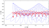Fig. 1 Orbital evolution of a deep MOND MLD-binary: the thick red curve shows the trajectory of the more massive particle with m1 = 2 M⊙, while the thin blue curve shows the trajectory of the less massive particle with m1 = 0.2 M⊙. The large red filled circle indicates the initial position of the more massive particle, the small blue filled circle the initial position of the less massive particle.

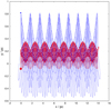Fig. 2 Orbital evolution of a deep MOND MLD-binary: shown is the complete orbital evolution over a period of 1 Gyr. Symbols and colour coding are identical to Fig. 1.

Fig. 3 Evolution of the linear momentum of a deep MOND MLD-binary: the slightly varying blue curve shows the MLD-linear momentum in Eq. (43) as a function of time. The strongly oscillating red curve shows the time evolution of the corresponding Newtonian linear momentum, $p_{\text{New\hspace{0.17em}}}=m_1{\dot{q}}_1+m_2{\dot{q}}_2$. Left: x-component of the linear momentum. Right: y-component of the linear momentum.

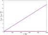Fig. 4 Centre of mass motions. The straight blue lines refer to the MLD-centre of mass (Eq. (46)) whereas the wobbling red curves show the Newtonian centre of mass, $R_{\text{com},\text{New}}=\frac{m_1{q}_1+m_2{q}_2}{m_1+m_2}$. The x-component of both centers of mass runs horizontally, the y-component increases continuously.

4.2 Binaries in an external galactic field

In the next test, the internally MONDian binary (from Sect. 4.1) is put on a circular orbit with radius R = 8300 pc in a flat rotation curve with v_c = 225 km/s = 230 pc/Myr. The external acceleration is a_ext = 6.37 pc/Myr² (Eq. (35)) and the corresponding Newtonian external acceleration is 𝑔_ext = 5.47 pc/Myr² (Eq. (36)); therefore, it is about two orders of magnitude larger than the internal acceleration. Adding the kinematical circular velocity of 230 pc/Myr to both components in Galactic tangential direction leads to a circular Galactic motion of the internally MONDian binary (Fig. 7), with one Galactic revolution within 227 Myr. The binary is integrated with no softening (ε = 0).

The MLD equation of motion of both binary components can be approximated by $$\mu \left(\frac{a_{\text{ext}}}{a_0}\right)a_1=\frac{G{m}_2}{{\left|r_2-r_1\right|}^2}\left(r_2-r_1\right)+g_{\text{ext}},$$(50) $$\mu \left(\frac{a_{\text{ext}}}{a_0}\right)a_2=-\frac{G{m}_1}{{\left|r_2-r_1\right|}^2}\left(r_2-r_1\right)+g_{\text{ext}},$$(51)

for cases where the external acceleration is very much larger than the internal acceleration, a_ext >> a_int.

For the acceleration of the Newtonian centre of mass follows $$\frac{m_1{a}_1+m_2{a}_2}{m_1+m_2}=\frac{g_{\text{ext}}}{\mu \left(a_{\text{ext}}/a_0\right)},$$(52)

and the radial acceleration is given by the scaled Newtonian acceleration.

In the next step, an internally Newtonian binary with the same components is set up with a semi-major axis of 2 × 10^–3 pc with the same tangential velocity of 230 pc/Myr. The binary does not move on a circular orbit as seen in Fig. 8. A circular MONDian velocity of 230 pc/Myr corresponds to a Newtonian circular velocity of 213 pc/Myr at a Galactocentric distance of 8300 pc. Now, the binary moves on a circular orbit (Fig. 9). An internally Newtonian binary follows a Newtonian orbit.

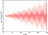Fig. 5 Evolution of the angular momentum of a deep MOND MLD-binary: the slightly varying blue curve shows the MLD-angular momentum (Eq. (47)) as a function of time. The strongly oscillating red curve shows the time evolution of the corresponding Newtonian angular momentum, $L_{\text{New\hspace{0.17em}}}=m_1{q}_1\times {\dot{q}}_1+m_2{q}_2\times {\dot{q}}_2$.

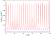Fig. 6 Evolution of the Hamiltonian of a deep MOND MLD-binary: the blue curve shows the MLD-Hamiltonian (Eq. (49)) as a function of time. The red curve shows the time evolution of the corresponding Newtonian-Hamiltonian, $H_{\text{New}}=\frac{p_1^2}{2m_1}+\frac{p_2^2}{2m_2}-G\frac{m_1{m}_2}{\left|q_2-q_1\right|}$.

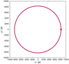Fig. 7 Binary in external field. The internally MONDian binary follows the MONDian Galactic orbit. The thick red curve shows the orbit of the 2 M⊙-component, the thin blue curve shows the orbit of the less massive star. The filled red circle marks the initial position of the binary.

4.3 Isolated hierarchical triple

In the next step, the equations of motion of an equal mass hierarchical triple are integrated in Newtonian dynamics and MLD, where the higher configuration is a MONDian binary with a semi-major axis of 1 pc and eccentricity e = 0. One component is a compact Newtonian binary with a semi-major axis of 10^–3 pc and eccentricity e = 0. All three components have equal masses, m₁ = m₂ = m₃ = 1 M_⊙. Thus, the internal Newtonian binary is an equal-mass binary, the outer one is a non-equalmass binary. The initial conditions of the compact binary are r₁ = (–0.333833, 0, 0) pc, v₁ = (0, –1.53826, 0) pc/Myr and r₂ = (–0.332833, 0, 0) pc, v₂ = (0, 1.46083, 0) pc/Myr. The initial conditions of the third body are r₃ = (0.666667, 0, 0) pc, v₂ = (0, 0.0774363, 0) pc/Myr. The initial conditions are such that the Newtonian centre of mass is initially at rest at the origin. The internal Newtonian acceleration of the compact binary is a_in = 4500 pc/Myr² = 1184 a₀. The acceleration of the less massive component of the outer binary is a_out = 0.009 pc/Myr² = 0.0024 a₀. The triple system is integrated for 100 Myr with no softening (ε = 0).

Figure 10 shows the orbital evolution of the triple system integrated in Newtonian dynamics. As expected both outer components move on circular orbits as it has no eccentricity. The centre of mass remains at rest. The evolution of the triple system in MLD is shown in Fig. 11. The orbital configuration now precesses around the origin. No net self-acceleration is visible.

Fig. 8 Binary in an external field. The internally Newtonian binary is set up with a MONDian rotational velocity. The thick red curve shows the orbit of the 2 M⊙ -component, the thin blue curve shows the orbit of the less massive star. The filled red circle marks the initial position of the binary.

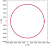Fig. 9 Binary in an external field. The internally Newtonian binary is set up with a Newtonian rotational velocity. The thick red curve shows the orbit of the 2 M⊙ -component, the thin blue curve shows the orbit of the less massive star. The filled red circle marks the initial position of the binary.

4.4 Isolated Plummer sphere

A Plummer sphere (Plummer 1911; Aarseth et al. 1974) is set up with n = 400 particles with masses of m_i = m₁ + (i – 1)∆m), equally distributed from m₁ = 0.1 M_Θ and m_u = 2 M_Θ, with a mass difference of ∆m = (m_u – m₁)/(n – 1). The total mass is M_tot = n(m_u + m_l)/2 = 420 M_⊙. Choosing a Plummer parameter of b = 3.1 pc the maximum internal acceleration is 0.076 pc/Myr² = 0.02 a₀. Figure 12 shows the evolution with time of the three spatial components of the Newtonian centre of mass. When the known conserved quantity in MLD is lacking, the MONDian simulation is compared with a Newtonian simulation with identical initial conditions.

In the general N -body case, it is currently not clear whether the MLD equations of motion can be derived from a variational principle and therefore the search for conserved quantities is much more difficult. However, a generalised expression of action equal reaction can be derived from Eq. (10) by multiplication with the mass of the considered particle and by subsequent summation over all particles: $${\displaystyle \sum _{i=1}^{i=N}{m}_i}\mu \left(\frac{\left|a_i\right|}{a_0}\right)a_i=G{\displaystyle \sum _{\begin{array}{c}j,i=0\\ j\ne i\end{array}}^{j,i=N}\frac{m_i{m}_j}{{\left|r_j-r_i\right|}^3}}\left(r_j-r_i\right)=0.$$(53)

In the Newtonian limit, the acceleration term can be expressed as the time derivative of the kinematical velocity $$0={\displaystyle \sum _{i=1}^{i=N}{m}_i}{a}_i={\displaystyle \sum _{i=1}^{i=N}{m}_i}{\stackrel{.}{v}}_i=\frac{d}{dt}{\displaystyle \sum _{i=1}^{i=N}{m}_i}{v}_i,$$(54)

thus, the total Newtonian linear momentum is conserved.

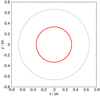Fig. 10 Triple in Newtonian dynamics. The inner thick (red) circle shows the orbit of the inner more massive binary. The thin (blue) outer circle shows the orbit of the single star.

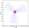Fig. 11 Triple in MLD. The inner thick (red) circle shows the orbit of the inner more massive binary. The thin (blue) outer circle shows the orbit of the single star.

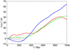Fig. 12 Centre of mass evolution of an isolated MLD-Plummer sphere: The thick lines show the x-(red), y-(green) and z-(blue)component of the Newtonian centre of mass evolution with time of an isolated Plummer sphere in MLD. The thin lines show the evolution of the Newtonian centre of mass of a Plummer sphere in Newtonian dynamics with identical initial conditions as the MLD-Plummer sphere (with identical colorcoding of the spatial components).

4.5 Comparison with deep MOND two-body expressions

Milgrom (2014, Eq. (23)) concluded that any MOND field theory leads to an internal force of an isolated two-body system with masses of m1 and m2 in the deep MOND limit of $$F=\frac{2\sqrt{a_{0}G}}{3r_{21}}\left({\left(m_1+m_2\right)}^{3/2}-m_1^{3/2}-m_2^{3/2}\right),$$(55)

where r₂₁ is the interparticle distance. Given that Newtonian momentum should be conserved in a MOND field theory (Bekenstein & Milgrom 1984) $m_1{\ddot{r}}_1=-m_2{\ddot{r}}_2$ the equations of motion of both particles are $${\stackrel{\mathrm{..}}{r}}_1=\frac{2\sqrt{a_{0}G}}{3m_1}\left({\left(m_1+m_2\right)}^{3/2}-m_1^{3/2}-m_2^{3/2}\right)\frac{r_2-r_1}{{\left|r_2-r_1\right|}^2}$$(56)

and $${\stackrel{\mathrm{..}}{r}}_2=\frac{2\sqrt{a_{0}G}}{3m_2}\left({\left(m_1+m_2\right)}^{3/2}-m_1^{3/2}-m_2^{3/2}\right)\frac{r_2-r_1}{{\left|r_2-r_1\right|}^2}.$$(57)

The evolution of the relative orbit is shown in Fig. 13 in comparison to the MLD equations for a duration of 20 Myr. In deep MOND, the binary following the Milgrom (2014) equations of motion displays a slower motion in radial direction, but precesses slightly faster than the MLD-binary.

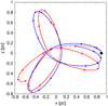Fig. 13 Deep MOND binary. Shown is the relative motion over 20 Myr of the isolated test binary with initial conditions (filled black circle) given at the beginning of Sect. 4.1 for three different sets of equations of motion: full MLD with transition function (red solid line), MLD in the deep MOND limit (Eqs. (39) and (40), light red line), and Milgrom’s formulation (blue solid line, Eqs. (56) and (57)). The small filled circles show the orbital positions in steps of 2 Myr.

5 Tidal tail simulations of open star clusters

To explore the difference in the dynamical formation and evolution of tidal tails of open star clusters, low-mass star cluster models are set up on a circular orbit in a Galactic field with a flat rotation curve. They are then integrated with the algorithm presented in Sect. 3.

5.1 Initial conditions

The model star clusters contain 400 equal-mass point particles with a mass of 0.5 M_Θ each, which are constant in time. Thus, stellar evolution is not included. Thus, all models have a total mass of 200 M_Θ. The particles are set up in phase space as a Plummer model (Plummer 1911; Aarseth et al. 1974) with a Plummer parameter of 3.1 pc. This corresponds to the properties of the current Hyades star cluster (Röser et al. 2019).

The initial position and velocity vectors of the star clusters are chosen such that their centre of mass orbits on a circular path with radius r₀ = 8300 pc in a flat rotation curve with 225 km/s, similar to the solar neighborhood, as used in related studies (Jerabkova et al. 2021; Pflamm-Altenburg et al. 2023).

The smoothing parameter is set to ε = 10^–3 pc. The difference between the softened and the unsoftened acceleration field of a particle with a mass of 0.5 M_Θ is shown in Fig. 14. The softened and the unsoftened acceleration fields start to diverge from each other at an acceleration of about 100 times higher than the MONDian threshold. The central particle density of the Plummer sphere is n₀ = (3N/4πb³) corresponding to a mean central inter particle distance of $\overline{d}\approx 0.7\text{pc}$. Therefore, we expect that (i) the driving long-distance encounters responsible for energy redistribution and the consequent evaporation of stars from the star cluster and (ii) the difference between MONDian and Newtonian dynamics below the acceleration threshold, a₀, are mostly unaffected by the gravitational softening.

To compare the MONDian and the Newtonian models using the same integrator, the threshold acceleration is a₀ = 3.8 Myr/pc² for the MONDian Models, and a₀ = 3.8 × 10^–20 Myr/pc² for the Newtonian models. In total, ten (five MONDian and five Newtonian) models were calculated. Two models (one Newtonian and one MONDian) were created with the same random seed and have identical initial conditions.

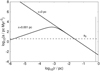Fig. 14 Softening. The Newtonian acceleration field of a star with a mass of 0.5 M⊙ is shown for the case of no softening (ε = 0 pc) and softening with a parameter of ε = 0.001 pc. The dashed horizontal line marks the MONDian acceleration threshold, a0. The vertical solid line indicates the mean central particle distance of ≈0.7 pc for a 400 particle Plummer sphere with Plummer parameter of 3.1 pc.

5.2 Time evolution of the orbital snapshots

The time evolution of one pair of star clusters in Newtonian and ML-dynamics is displayed in Fig. 15 at 0 Myr, in Fig. 16 after 250 Myr, in Fig. 17 after 500 Myr, in Fig. 18 after 750 Myr, and in Fig. 19 after 1000 Myr. To compare the relative positions of the star clusters in Newtonian and ML-dynamics, the arrows indicating the direction of the Galactic rotation and the direction to the Galactic centre and the corresponding labels are located at the same position. The short dashed line indicates the path from the Galactic centre to the density centre of the star cluster and the solid curved line shows the circular orbit.

The star clusters orbit anti-clockwise. The inner arm is the leading arm, the outer arm is the trailing arm. In the Newtonian case both tidal arms are approximately equally populated. In the MLD case the tidal tails are populated asymmetrically. The leading tidal arm contains continuously more members than the trailing arm.

Simultaneously to the asymmetric population of the tidal arms in ML-dynamics, the star cluster follows the Newtonian star cluster. This can be seen in the larger separation between the arrow pointing towards the Galactic centre and the connecting (dashed) line between the Galactic centre and the density centre of the star cluster in the MLD case than in the Newtonian case.

This might be due to some kind of local conservation of linear momentum. As more stars end up in the leading tail, more momentum is carried away from the star cluster into the moving direction of the star cluster. Thus, the star cluster is expected to get a low recoil. However (as pointed out in Sect. 2), a concept akin to linear momentum conservation (as in Newtonian dynamics) does not exist in Milgrom-law dynamics, yet. Further theoretical work is required to explore the conservation of dynamical quantities in MLD.

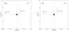Fig. 15 Orbital snapshots at 0 Myr. Star cluster evolution in Newtonian (left) and discrete Milgrom-law Dynamics (right). See Sect. 5.2 for details.

Fig. 16 Same as Fig. 15 but at 250 Myr.

5.3 Analyzing the tidal tails

The criteria used to establish whether or not a star is considered to be a member of the star cluster or of the leading or trailing tidal arm is the same as the method applied in Pflamm-Altenburg et al. (2023). If the distance of a star to the centre of the star cluster is less than a cut-off radius (here, 10 pc), then the star is considered to be a member of the star cluster. If this distance is larger than 10 pc, then the star is considered to be a member of one tidal arm. If the angle between the distance vector of the particular star to the star cluster centre and the velocity vector of the star cluster is less than 90°, then the star is considered to be a member of the leading tidal arm. If this angle is larger than 90°, the star is assigned to the trailing arm.

In Pflamm-Altenburg et al. (2023), the stochastic asymmetry of tidal tails in Newtonian dynamics was quantified using test particle calculations in an analytic Plummer potential orbiting the Galactic centre. The origin of the Plummer potential has been used as the cluster centre. In the current work, the cluster centre had to be determined by the positions of all particles following standard procedures. A local density was assigned to each particle using the sixth nearest neighbour method (Casertano & Hut 1985). In the next step, the density centre was generally calculated by the weighted sum of all local particle densities (Aarseth 2003). This method requires the systems to have a nearly spherical symmetry. However, due to the asymmetric tidal tails, this requirement was not met. Therefore, we first determined the position of maximum density, expected to be located close to the centre of the star cluster. Then, only those particles lying within a sphere with 10 pc radius, where the position of maximum density is at the centre, will be considered for the calculation of the density centre.

5.4 Time evolution of the asymmetry of the tidal tails

The asymmetry of the tidal arms at a time, t, is calculated as $$ϵ=\frac{n_1-n_{\text{t}}}{n_{\text{l}}+n_{\text{t}}},$$(58)

where n₁ is the number of stars in the leading arm and n_t is the number of stars in the trailing arm at time t (Pflamm-Altenburg et al. 2023). Thus, for ϵ > 0, the leading arm contains more members than the trailing arm. Figure 20 shows the evolution of the asymmetry of all 10 simulations. It can be seen that in both dynamical contexts the mean asymmetry is positive, the leading arm contains more members than the trailing arm. However, in MONDian dynamics the mean asymmetry varies between 0.2 to 0.3; whereas in Newtonian dynamics the mean asymmetry decreases continuously and gradually below 0.1.

A comparison of the asymmetry of the simulated star clusters with observed star clusters requires that all tidal tail stars of a star cluster can be identified among the field stars. This becomes more difficult with increasing distance of a tidal tail star to the parent star cluster. Therefore, Kroupa et al. (2022) considered only stars within a 50–200 pc distance to the star cluster and introduced the q-parameter $$q=\frac{N_{1,50-200\text{pc}}}{N_{\text{t},50-200\text{pc}}},$$(59)

where N_{1,50–200 pc} is the number of stars in the leading arm in the considered distance range and N_{t,50–200 pc} the respective number of stars in the trailing arm. For a q-parameter q > 1 the leading arm contains more members than the trailing arm in the respective distance range.

The evolution of the q-parameter can be seen in Fig. 21. In MOND, the q-parameter varies between 1.5 and 2. The leading arm contains more stars than the trailing arm. In contrast, in Newtonian dynamics the q-parameter finally stays constant around 1 and the tidal tails show no asymmetry.

Fig. 17 Same as Fig. 15 but at 500 Myr.

Fig. 18 Same as Fig. 15 but at 750 Myr.

Fig. 19 Same as Fig. 15 but at 1000 Myr.

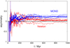Fig. 20 Asymmetry of tidal arms. Thin lines show the evolution of the asymmetry of the ten individual simulations: five Newtonian (red) and five MONDian (blue) simulations. The thick lines show the arithmetic mean values.

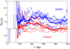Fig. 21 q parameter. Thin lines show the evolution of the q parameter of the ten individual simulations, five Newtonian (red) and five MONDian (blue) simulations. The thick lines show the arithmetic mean values.

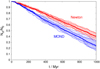Fig. 22 Evolution of the cluster member number fraction. Each of the ten models, five Newtonian (red) and five MONDian (blue) models, are shown as thin solid lines. The evolution of the mean values are given by thick solid lines. The light-blue and the light-red areas indicate the 1σ region around the mean value.

5.5 Evaporation rate

The number of stars within the constant evaporation radius of 10pc decrease differently fast in both dynamical theories as shown in Fig. 22. In the MOND model, the mean ratio of the current number to the initial number of cluster members after 1 Gyr is 0.26 with a 1σ variance of 0.07. Thus, 74% of the initial stars have already evaporated from the cluster. For 400 initial stars the evaporation rate in the MOND case is 0.296 stars/Myr or one star every 3.4 Myr.

The star cluster evaporates slower in the pure Newtonian case. After 1 Gyr of evolution the mean remaining cluster fraction is 0.41 with a 1σ variance of 0.06. Here, only 59% of all stars have evaporated from the star cluster within 1 Gyr. The evaporation rate is 0.236 stars/Myr or one star every 4.2 Myr. The evaporation rate in the MONDian case is about 25% higher than in the Newtonian case.

This can be understood by the increased effective internal gravitational constant. The external kinematical acceleration of a flat rotation curve with 225 km/s = 230 pc/Myr at a distance of 8300 pc from the galaxy centre is a_ext = 6.4pc/Myr.

For a mass of ≈200 M_⊙ and Plummer parameter b = 3.1 pc the internal maximal acceleration is 0.036 pc/Myr² . Therefore, the internal dynamics is to first order Newtonian with a gravitational constant increased by a factor of µ(a_ext/a₀)^–1 = 1.16. From Baumgardt & Makino (2003, Eq. (5)) it is derived that the dissolution time scale, T_diss , of a star cluster in Newtonian dynamics scales inversely with the square root of the gravitational constant, T_diss ∝ G^–1/2. The ratio of the dissolution time scales in the Newtonian case, T_diss , and in MLD in case of the external field effect, T_diss,EFE, is $$\frac{T_{\text{diss},\text{EFE}}}{T_{\text{diss}}}=\sqrt{\frac{G}{G_{\text{EFE}}}}=\sqrt{\mu \left(a_{\text{ext}}/a_0\right)}=\mathrm{0.93.}$$(60)

The ratio of the numerical dissolution time scale of the models here is approximately $$\frac{T_{\text{diss},\text{EFE}}}{T_{\text{diss}}}=\frac{\dot{N}}{{\dot{N}}_{\text{MLD}}}=\frac{0.236}{0.296}=0.8,$$(61)

and is about 10% smaller than expected from the EFE approximation.

6 Conclusions

Direct N-body simulations of star clusters are performed in a MONDian dynamical context. For this Milgrom’s law has been postulated to be valid for arbitrary N -body systems. In comparison to Newton models, two main differences emerge: (i) the tidal arms are asymmetrically populated and the leading tidal arm contains significantly more stars than the trailing arm; (ii) the star cluster evaporates stars or dissolves at a significantly faster rate.

It is clear that asymmetric tidal tails arise in two different types of MONDian dynamics, namely, in QUMOND (Thomas et al. 2018; Kroupa et al. 2022) and Milgrom-law dynamics (this work). This leads to the conclusion that this effect is a property of the general MONDian dynamical concept, rather than a result of a specific detailed realisation.

However, the application of Milgrom’s law to the dynamics of discrete N-body systems is limited to systems which are internally not Newtonian if embedded in an external MONDian field. This is artificially achieved here by softening the two-body force. Generalised Newtonian equations of motion should internally already contain the non-Newtonisation of centre of mass motions of compact subsystems, if constructible at all, which needs to be explored.

However, to simulate the dynamical evolution of non-relaxed discrete systems, such as open star clusters or wide binaries, the development of collisional direct N -body codes is required, as collision-less methods are not suitable for modelling these kinds of systems.

This can be done by deriving mathematically consistent equations of motions for point-mass systems from MOND field theories like AQUAL and QUMOND. However, due to the inherent non-linearity, this is very difficult to achieve. An alternative approach would be to extend the Newtonian equations of motions in such a way that all necessary conditions of MOND-type theories would be fulfilled. Both strategies establish a complete new field of research. Finally, because open star clusters are nearby systems they are very well accessible via astrometric observations. In addition, they are ideal test objects to discriminate between the validity of Newtonian or MONDian dynamics on parsec scales.

Acknowledgements

J.P.A. acknowledges permanent hospitality by the Helmholtz-Institut für Strahlen- und Kernphysik.

References

All Figures

Fig. 1 Orbital evolution of a deep MOND MLD-binary: the thick red curve shows the trajectory of the more massive particle with m1 = 2 M⊙, while the thin blue curve shows the trajectory of the less massive particle with m1 = 0.2 M⊙. The large red filled circle indicates the initial position of the more massive particle, the small blue filled circle the initial position of the less massive particle.

In the text

	Fig. 2 Orbital evolution of a deep MOND MLD-binary: shown is the complete orbital evolution over a period of 1 Gyr. Symbols and colour coding are identical to Fig. 1.
In the text

Fig. 3 Evolution of the linear momentum of a deep MOND MLD-binary: the slightly varying blue curve shows the MLD-linear momentum in Eq. (43) as a function of time. The strongly oscillating red curve shows the time evolution of the corresponding Newtonian linear momentum, $p_{\text{New\hspace{0.17em}}}=m_1{\dot{q}}_1+m_2{\dot{q}}_2$. Left: x-component of the linear momentum. Right: y-component of the linear momentum.

In the text

	Fig. 4 Centre of mass motions. The straight blue lines refer to the MLD-centre of mass (Eq. (46)) whereas the wobbling red curves show the Newtonian centre of mass, $R_{\text{com},\text{New}}=\frac{m_1{q}_1+m_2{q}_2}{m_1+m_2}$. The x-component of both centers of mass runs horizontally, the y-component increases continuously.
In the text

	Fig. 5 Evolution of the angular momentum of a deep MOND MLD-binary: the slightly varying blue curve shows the MLD-angular momentum (Eq. (47)) as a function of time. The strongly oscillating red curve shows the time evolution of the corresponding Newtonian angular momentum, $L_{\text{New\hspace{0.17em}}}=m_1{q}_1\times {\dot{q}}_1+m_2{q}_2\times {\dot{q}}_2$.
In the text

	Fig. 6 Evolution of the Hamiltonian of a deep MOND MLD-binary: the blue curve shows the MLD-Hamiltonian (Eq. (49)) as a function of time. The red curve shows the time evolution of the corresponding Newtonian-Hamiltonian, $H_{\text{New}}=\frac{p_1^2}{2m_1}+\frac{p_2^2}{2m_2}-G\frac{m_1{m}_2}{\left|q_2-q_1\right|}$.
In the text

	Fig. 7 Binary in external field. The internally MONDian binary follows the MONDian Galactic orbit. The thick red curve shows the orbit of the 2 M⊙-component, the thin blue curve shows the orbit of the less massive star. The filled red circle marks the initial position of the binary.
In the text

	Fig. 8 Binary in an external field. The internally Newtonian binary is set up with a MONDian rotational velocity. The thick red curve shows the orbit of the 2 M⊙ -component, the thin blue curve shows the orbit of the less massive star. The filled red circle marks the initial position of the binary.
In the text

	Fig. 9 Binary in an external field. The internally Newtonian binary is set up with a Newtonian rotational velocity. The thick red curve shows the orbit of the 2 M⊙ -component, the thin blue curve shows the orbit of the less massive star. The filled red circle marks the initial position of the binary.
In the text

	Fig. 10 Triple in Newtonian dynamics. The inner thick (red) circle shows the orbit of the inner more massive binary. The thin (blue) outer circle shows the orbit of the single star.
In the text

	Fig. 11 Triple in MLD. The inner thick (red) circle shows the orbit of the inner more massive binary. The thin (blue) outer circle shows the orbit of the single star.
In the text

Fig. 12 Centre of mass evolution of an isolated MLD-Plummer sphere: The thick lines show the x-(red), y-(green) and z-(blue)component of the Newtonian centre of mass evolution with time of an isolated Plummer sphere in MLD. The thin lines show the evolution of the Newtonian centre of mass of a Plummer sphere in Newtonian dynamics with identical initial conditions as the MLD-Plummer sphere (with identical colorcoding of the spatial components).

In the text

Fig. 13 Deep MOND binary. Shown is the relative motion over 20 Myr of the isolated test binary with initial conditions (filled black circle) given at the beginning of Sect. 4.1 for three different sets of equations of motion: full MLD with transition function (red solid line), MLD in the deep MOND limit (Eqs. (39) and (40), light red line), and Milgrom’s formulation (blue solid line, Eqs. (56) and (57)). The small filled circles show the orbital positions in steps of 2 Myr.

In the text

Fig. 14 Softening. The Newtonian acceleration field of a star with a mass of 0.5 M⊙ is shown for the case of no softening (ε = 0 pc) and softening with a parameter of ε = 0.001 pc. The dashed horizontal line marks the MONDian acceleration threshold, a0. The vertical solid line indicates the mean central particle distance of ≈0.7 pc for a 400 particle Plummer sphere with Plummer parameter of 3.1 pc.

In the text

	Fig. 15 Orbital snapshots at 0 Myr. Star cluster evolution in Newtonian (left) and discrete Milgrom-law Dynamics (right). See Sect. 5.2 for details.
In the text

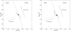	Fig. 16 Same as Fig. 15 but at 250 Myr.
In the text

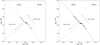	Fig. 17 Same as Fig. 15 but at 500 Myr.
In the text

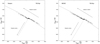	Fig. 18 Same as Fig. 15 but at 750 Myr.
In the text

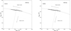	Fig. 19 Same as Fig. 15 but at 1000 Myr.
In the text

	Fig. 20 Asymmetry of tidal arms. Thin lines show the evolution of the asymmetry of the ten individual simulations: five Newtonian (red) and five MONDian (blue) simulations. The thick lines show the arithmetic mean values.
In the text

	Fig. 21 q parameter. Thin lines show the evolution of the q parameter of the ten individual simulations, five Newtonian (red) and five MONDian (blue) simulations. The thick lines show the arithmetic mean values.
In the text

	Fig. 22 Evolution of the cluster member number fraction. Each of the ten models, five Newtonian (red) and five MONDian (blue) models, are shown as thin solid lines. The evolution of the mean values are given by thick solid lines. The light-blue and the light-red areas indicate the 1σ region around the mean value.
In the text

References

- Aarseth, S. J. 1963, MNRAS, 126, 223 [NASA ADS] [Google Scholar]
- Aarseth, S. J. 2003, Gravitational N-Body Simulations, ed. S. J. Aarseth, (Cambridge, UK: Cambridge University Press), 430 [Google Scholar]
- Aarseth, S. J., Henon, M., & Wielen, R. 1974, A&A, 37, 183 [NASA ADS] [Google Scholar]
- Amorisco, N. C., Gómez, F. A., Vegetti, S., & White, S. D. M. 2016, MNRAS, 463, L17 [Google Scholar]
- Aprile, E., Aalbers, J., Agostini, F., et al. 2020, Phys. Rev. D, 102, 072004 [CrossRef] [Google Scholar]
- Aprile, E., Abe, K., Agostini, F., et al. 2022, Phys. Rev. Lett., 129, 161805 [CrossRef] [PubMed] [Google Scholar]
- Barrena, R., Biviano, A., Ramella, M., Falco, E. E., & Seitz, S. 2002, A&A, 386, 816 [NASA ADS] [CrossRef] [EDP Sciences] [Google Scholar]
- Baumgardt, H., & Makino, J. 2003, MNRAS, 340, 227 [NASA ADS] [CrossRef] [Google Scholar]
- Bekenstein, J., & Milgrom, M. 1984, ApJ, 286, 7 [NASA ADS] [CrossRef] [Google Scholar]
- Bertone, G., & Hooper, D. 2018, Rev. Mod. Phys., 90, 045002 [NASA ADS] [CrossRef] [Google Scholar]
- Boffin, H. M. J., Jerabkova, T., Beccari, G., & Wang, L. 2022, MNRAS, 514, 3579 [NASA ADS] [CrossRef] [Google Scholar]
- Bonaca, A., Pearson, S., Price-Whelan, A. M., et al. 2020, ApJ, 889, 70 [NASA ADS] [CrossRef] [Google Scholar]
- Bosma, A. 1981, AJ, 86, 1825 [NASA ADS] [CrossRef] [Google Scholar]
- Casertano, S., & Hut, P. 1985, ApJ, 298, 80 [Google Scholar]
- Clowe, D., Bradac?, M., Gonzalez, A. H., et al. 2006, ApJ, 648, L109 [NASA ADS] [CrossRef] [Google Scholar]
- Drees, M. 2019, PoS, ICHEP2018, 730 [Google Scholar]
- Erkal, D., Koposov, S. E., & Belokurov, V. 2017, MNRAS, 470, 60 [NASA ADS] [CrossRef] [Google Scholar]
- Ettori, S., Donnarumma, A., Pointecouteau, E., et al. 2013, Space Sci. Rev., 177, 119 [Google Scholar]
- Famaey, B., & McGaugh, S. S. 2012, Liv. Rev. Relativ., 15, 10 [Google Scholar]
- Felten, J. E. 1984, ApJ, 286, 3 [NASA ADS] [CrossRef] [Google Scholar]
- Fukushige, T., & Heggie, D. C. 2000, MNRAS, 318, 753 [CrossRef] [Google Scholar]
- Hut, P., Makino, J., & McMillan, S. 1995, ApJ, 443, L93 [NASA ADS] [CrossRef] [Google Scholar]
- Ibata, R. A., Lewis, G. F., Thomas, G., Martin, N. F., & Chapman, S. 2017, ApJ, 842, 120 [NASA ADS] [CrossRef] [Google Scholar]
- Jerabkova, T., Boffin, H. M. J., Beccari, G., et al. 2021, A&A, 647, A137 [NASA ADS] [CrossRef] [EDP Sciences] [Google Scholar]
- Knebe, A., & Gibson, B. K. 2004, MNRAS, 347, 1055 [NASA ADS] [CrossRef] [Google Scholar]
- Kokubo, E., Yoshinaga, K., & Makino, J. 1998, MNRAS, 297, 1067 [NASA ADS] [CrossRef] [Google Scholar]
- Kroupa, P., Jerabkova, T., Thies, I., et al. 2022, MNRAS, 517, 3613 [CrossRef] [Google Scholar]
- Küpper, A. H. W., Kroupa, P., Baumgardt, H., & Heggie, D. C. 2010, MNRAS, 401, 105 [Google Scholar]
- Lüghausen, F., Famaey, B., & Kroupa, P. 2015, Can. J. Phys., 93, 232 [CrossRef] [Google Scholar]
- Makino, J. 1991, ApJ, 369, 200 [Google Scholar]
- Markevitch, M., Gonzalez, A. H., David, L., et al. 2002, ApJ, 567, L27 [Google Scholar]
- Milgrom, M. 1983a, ApJ, 270, 371 [Google Scholar]
- Milgrom, M. 1983b, ApJ, 270, 384 [Google Scholar]
- Milgrom, M. 1983c, ApJ, 270, 365 [Google Scholar]
- Milgrom, M. 1999, Phys. Lett. A, 253, 273 [NASA ADS] [CrossRef] [Google Scholar]
- Milgrom, M. 2010, MNRAS, 403, 886 [NASA ADS] [CrossRef] [Google Scholar]
- Milgrom, M. 2014, Phys. Rev. D, 89, 024016 [NASA ADS] [CrossRef] [Google Scholar]
- Nusser, A. 2002, MNRAS, 331, 909 [NASA ADS] [CrossRef] [Google Scholar]
- Pearson, S., Price-Whelan, A. M., & Johnston, K. V. 2017, Nat. Astron., 1, 633 [NASA ADS] [CrossRef] [Google Scholar]
- Pflamm-Altenburg, J., Kroupa, P., Thies, I., et al. 2023, A&A, 671, A88 [NASA ADS] [CrossRef] [EDP Sciences] [Google Scholar]
- Pinfield, D. J., Jameson, R. F., & Hodgkin, S. T. 1998, MNRAS, 299, 955 [NASA ADS] [CrossRef] [Google Scholar]
- Plummer, H. C. 1911, MNRAS, 71, 460 [Google Scholar]
- Read, J. I., Wilkinson, M. I., Evans, N. W., Gilmore, G., & Kleyna, J. T. 2006, MNRAS, 367, 387 [NASA ADS] [CrossRef] [Google Scholar]
- Röser, S., Schilbach, E., & Goldman, B. 2019, A&A, 621, L2 [NASA ADS] [CrossRef] [EDP Sciences] [Google Scholar]
- Rubin, V. C., Ford, W. K., J., & Thonnard, N. 1978, ApJ, 225, L107 [NASA ADS] [CrossRef] [Google Scholar]
- Teyssier, R. 2002, A&A, 385, 337 [CrossRef] [EDP Sciences] [Google Scholar]
- Thomas, G. F., Famaey, B., Ibata, R., et al. 2018, A&A, 609, A44 [NASA ADS] [CrossRef] [EDP Sciences] [Google Scholar]
- Tiongco, M. A., Vesperini, E., & Varri, A. L. 2016, MNRAS, 461, 402 [NASA ADS] [CrossRef] [Google Scholar]