| Issue |
A&A
Volume 693, January 2025
|
|
|---|---|---|
| Article Number | A190 | |
| Number of page(s) | 12 | |
| Section | Extragalactic astronomy | |
| DOI | https://doi.org/10.1051/0004-6361/202346239 | |
| Published online | 17 January 2025 | |
ALMA Lensing Cluster Survey: Dust mass measurements as a function of redshift, stellar mass, and star formation rate from z = 1 to z = 5
1
Max-Planck-Institut für extraterrestrische Physik, 85748 Garching, Germany
2
Department of Space, Earth and Environment, Chalmers University of Technology, SE-412 96 Gothenburg, Sweden
3
Aix Marseille Université, CNRS, CNES, LAM (Laboratoire d’Astrophysique de Marseille), UMR 7326, 13388 Marseille, France
4
Astronomy Department, Universidad de Concepción, Barrio Universitario S/N, Concepción, Chile
5
Cosmic Dawn Center (DAWN), Copenhagen, Denmark
6
Niels Bohr Institute, University of Copenhagen, Jagtvej 128, DK-2200 Copenhagen N, Denmark
7
Institute of Astronomy, Graduate School of Science, The University of Tokyo, 2-21-1 Osawa, Mitaka, Tokyo 181-0015, Japan
8
Research Center for the Early Universe, Graduate School of Science, The University of Tokyo, 7-3-1 Hongo, Bunkyo-ku, Tokyo 113-0033, Japan
9
Kapteyn Astronomical Institute, University of Groningen, PO Box 800 9700 AV Groningen, The Netherlands
10
International Centre for Radio Astronomy Research (ICRAR), M468, University of Western Australia, 35 Stirling Hwy, Crawley, WA 6009, Australia
11
Instituto de Astrofísica, Facultad de Física, Pontificia Universidad Católica de Chile, Campus San Joaquín, Av. Vicuña Mackenna 4860, 7820436 Macul Santiago, Chile
12
Centro de Astroingeniería, Facultad de Física, Pontificia Universidad Católica de Chile, Campus San Joaquín, Av. Vicuña Mackenna 4860, 7820436 Macul Santiago, Chile
13
Millennium Institute of Astrophysics, Nuncio Monseñor Sótero Sanz 100, Of 104, Providencia, Santiago, Chile
14
Observatoire de Genève, Université de Genève, 51 Ch. des Maillettes, 1290 Versoix, Switzerland
15
Departamento de Física Teórica y del Cosmos, Campus de Fuentenueva, Edificio Mecenas, Universidad de Granada, E-18071 Granada, Spain
16
Instituto Carlos I de Física Teórica y Computacional, Facultad de Ciencias, E-18071 Granada, Spain
17
Space Telescope Science Institute, 3700 San Martin Dr., Baltimore, MD 21218, USA
18
CRAL, Observatoire de Lyon, Université Lyon 1, 9 Avenue Ch. André, F-69561 Saint Genis Laval Cedex, France
19
Steward Observatory, University of Arizona, 933 N. Cherry Avenue, Tucson 85721, USA
20
Space Telescope Science Institute, 3700 San Martin Dr., Baltimore, MD 21218, USA
21
Department of Physics & Astronomy, Johns Hopkins University, 3400 N Charles St, Baltimore, MD 21218, USA
⋆ Corresponding author; jbjolly@mpe.mpg.de
Received:
24
February
2023
Accepted:
15
November
2024
Context. Understanding the dust content of galaxies, its evolution with redshift and its relation to stars and star formation is fundamental for our understanding of galaxy evolution. Dust acts as a catalyst of star formation and as a shield for star light. Advanced millimeter facilities like ALMA have made dust observation ever more accessible, even at high redshift. However, dust emission is typically very faint, making the use of stacking techniques is instrumental in the study of dust in statistically sound samples.
Aims. Using the ALMA Lensing Cluster Survey (ALCS) wide-area band-6 continuum dataset (∼ 110 arcmin2 across 33 lensing clusters), we constrain the dust-mass evolution with redshift, stellar mass, and star formation rate (SFR).
Methods. After binning sources according to redshift, SFR, and stellar mass as extracted from an HST-IRAC catalog, we performed a set of continuum-stacking analyses in the image domain using LINESTACKER on sources between z = 1 and z = 5, which further improved the depth of our data. The large field of view provided by the ALCS allowed us to reach a final sample of ∼4000 galaxies with known coordinates and SED-derived physical parameters. We stacked sources with an SFR between 10−3 and 103 M⊙ per year and a stellar mass between 108 and 1012 M⊙, and we split them into different stellar mass and SFR bins. Through stacking, we retrieved the continuum 1.2 mm flux, which is a known dust-mass tracer. This allowed us to derive the dust-mass evolution with redshift and its relation to the SFR and stellar mass.
Results. We clearly detect the continuum in most of the subsamples. From the nondetections, we derive 3σ upper limits. We observe a steady decline in the average dust mass with redshift. Moreover, sources with a higher stellar mass or SFR have a higher dust mass on average. This allows us to derive scaling relations. Our results mostly agree well with models at z ∼ 1–3, but they indicate a typically lower dust mass than predicted at higher redshift.
Key words: dust / extinction / galaxies: evolution / galaxies: ISM / galaxies: statistics
© The Authors 2025
 Open Access article, published by EDP Sciences, under the terms of the Creative Commons Attribution License (https://creativecommons.org/licenses/by/4.0), which permits unrestricted use, distribution, and reproduction in any medium, provided the original work is properly cited.
This article is published in open access under the Subscribe to Open model.
Open Access funding provided by Max Planck Society.
1. Introduction
Dust impacts the direct evolution of galaxies and their observations in multiple ways. It is thought to be the main catalyst of H2 formation (Wakelam et al. 2017), which is one of the main components of molecular clouds in the interstellar medium (ISM), and hence, it is one of the principal drivers of star formation (e.g. Scoville 2013). In addition to the direct effect on the physical properties of galaxies, dust also plays a critical role in astrophysical observations. The dust grains attenuating the starlight are consequently heated, and they in turn reradiate the energy at longer wavelengths. This is the so-called dust-obscured star formation (see for e.g. Casey et al. 2014; Hodge & da Cunha 2020; Zavala et al. 2021). As a consequence, the light from star-forming regions is typically dominated by dust continuum emission. The relation between dust mass and other physical characteristics of galaxies have been intensely studied, for example, through the dust-to-gas (atomic and molecular) or dust-to-metal ratios (e.g. Hunt et al. 2005; Draine et al. 2007; Engelbracht et al. 2008; Galametz et al. 2011; Magrini et al. 2011; Saintonge et al. 2013; Rémy-Ruyer et al. 2014; Combes 2018; Li et al. 2019; Shapley et al. 2020; Tacconi et al. 2020; Birkin et al. 2021; Popping & Péroux 2022; Popping et al. 2023), or through the ratio of the dust mass versus star formation rate (SFR) (e.g. da Cunha et al. 2010; Casey 2012; Santini et al. 2014; Dudzevičiūtė et al. 2020, 2021).
Recent studies have shown that the proportion of dust-obscured star formation has evolved with redshift (Bouwens et al. 2020). It has been estimated to be a dominant fraction during the peak of the cosmic star formation history. However, it appears to have accounted for only ∼20%–25% of the total star formation at redshift z = 6–7 (see Zavala et al. 2021). Similarly, the overall cosmic dust density has been shown to peak around z ∼ 1 − 2 and to rapidly decline at higher redshift (see for example Driver et al. 2018; Magnelli et al. 2020; Pozzi et al. 2020; Dudzevičiūtė et al. 2021). Furthermore, massive dust reservoirs have been detected in massive high-redshift galaxies (e.g. Bertoldi et al. 2003; Valiante et al. 2009; Venemans et al. 2012; Watson et al. 2015; Laporte et al. 2017; Tamura et al. 2019, 2023). While this is probably not the case for the more typical less massive high-redshift galaxies, it highlights the importance of studying the evolution of dust mass with redshift.
Millimeter (mm) or submillimeter (submm) emission was proposed to be a tracer of dust mass (Scoville et al. 2014, 2016, 2017), with the assumption that the emission is optically thin and measured far from the peak of the spectral energy distribution of the dust. The Atacama Large Millimeter/Submillimeter Array (ALMA) has become instrumental in the quest to study the dust mass in lower-mass galaxies and its evolution in the mm and submm bands. With large surveys and high-redshift single-target observations becoming progressively more accessible (e.g. Knudsen et al. 2016; Walter et al. 2016; González-López et al. 2017, 2020; Laporte et al. 2017; Béthermin et al. 2020; Aravena et al. 2020), the evolution of dust is studied in increasingly statistically sound samples.
However, observations of high-redshift galaxies are typically biased by construction toward the observation of the brightest sources (Malmquist bias). To draw a complete picture of the dust evolution with redshift, it is necessary to also study galaxies with lower intrinsic luminosities. Gravitational lensing can be used as a tool to enhance the signal from faint galaxies without the need for excessive integration time. Similarly, tools such as stacking can statistically drastically improve the signal-to-noise ratio (S/N) for large samples. With the help of gravitational lensing and stacking, it is hence possible to push the limit of observations toward sources with a lower intrinsic dust luminosity.
We present the stacking analysis of 10386 gravitationally lensed galaxies from the ALMA Lensing Cluster Survey (ALCS) at z > 1 (cluster and field sources at z ≲ 1 are studied in a separate paper; Guerrero et al. (2023). By binning galaxies by redshift and further splitting them according to their stellar mass or SFR, we study the evolution of the dust mass with redshift and its scaling relation with stellar mass and SFR. We also integrate the contribution from all galaxies in each redshift bin to assess the evolution of the cosmic dust density.
In Sect. 2 we describe the overall data set, the catalog, and the different subsamples. In Sect. 3 we describe the stacking method, which we performed using LINESTACKER (Jolly et al. 2020), and the processes involved in the dust-mass calculation. In Sect. 4 we present our results, and we discuss them in Sect. 5. Finally, in Sect. 6 we summarize this paper. In the appendix (available on Zenodo), we show alternative stacking procedures as well as some additional details for the main analysis.
Throughout the paper, we assume a ΛCDM cosmology with Ωm = 0.3, Ωλ = 0.7 and H0 = 70 km s−1 Mpc−3. All magnitudes are quoted in the AB system, such that MAB = 23.9–2.5 log10 (Sν [μJy]).
2. Data and sample
2.1. ALCS
The ALCS is a large ALMA program that was accepted in cycle 6 (Project ID: 2018.1.00035.L; PI: K. Kohno). It observed 33 lensing clusters in band 6 (λ ∼ 1.2 mm), which spanned ∼ 110 arcmin2 (primary beam (PB) > 0.5). The clusters are distributed as follows: 16 clusters were taken from RELICS (the Reionization Lensing Cluster Survey; Coe et al. 2019), 12 clusters were taken from CLASH (the Cluster Lensing And Supernova survey with Hubble; Postman et al. 2012), and 5 clusters were taken from the Frontier Fields survey (Lotz et al. 2017). The observations were carried out between December 2018 and December 2019 (cycles 6 and 7) in compact-array configurations C43-1 and C43-2 in a double-frequency window setup. The observations were made from 250.0 to 257.5 GHz and from 265.0 to 272.5 GHz for a total bandwidth of 15 GHz. When available, the ALCS data were concatenated with existing ALMA data, notably the ALMA Frontier Fields Survey (Project ID: 2013.1.00999.S, PI: Bauer and Project ID; 2015.1.01425.S: PI: Bauer). The data were reduced and calibrated using the Common Astronomy Software Applications (CASA, McMullin et al. 2007) package version 5.4.0 for the 26 clusters observed in cycle 6 and with v5.6.1 for the remaining clusters that were observed in cycle 7. Throughout this paper, we use natural weighted primary-beam-corrected and uv-tapered continuum maps, with a tapering parameter of 2 arcsec (the full width at half maximum of the synthesized beam is 2 arcsec; with a corresponding pixel size of 0.16 arcsec). uv-tapered maps were chosen over natural resolution maps to ensure the beam-size homogeneity of the different images when stacking. The average root mean square (RMS) of the maps is ∼63 μJy/beam (see Table 1 for the detailed RMS of each map). A full description of the survey can be found in Kohno et al. (2023).
Number of stacked sources in each cluster, and the map RMS.
2.2. Source catalog
We extracted the positions, redshifts, physical characteristics (SFRs and stellar masses) and lensing magnifications of galaxies at 1 ≤ z ≤ 5 from the Hubble Space Telescope (HST)-Infrared Array Camera (IRAC) catalog presented in Kokorev et al. (2022). When available, spectroscopic redshifts were used in place of photometric redshifts. While the SFRs and stellar masses extracted from the Kokorev et al. (2022) catalog are not corrected for magnification, the SFRs and stellar masses presented in this paper are always the intrinsic ones, that is, they are corrected for magnification.
We selected only the sources from the full catalog (the number of remaining sources is indicated after each step) that (i) had defined redshifts and magnifications and were not tagged as poor photometry (bad_phot ≠1), that is, 1 888 977; (ii) had redshift uncertainties (|z160 − z840|) below 0.4, that is, 76728; (iii) had 108 ≤ M*/M⊙ ≤ 1012 and 0.001 ≤ SFR/(M⊙/year)≤103, that is, 51355; (iv) had H-band magnitudes above 24, to avoid contamination from blue faint galaxies, that is, 50 983; (v) had associated PB values higher than 0.5, that is, 13 403; (vi) had a z < 5, that is, 12 980; (vii) had a magnification factor below 100, that is, 12 967; and that (viii) had a z ≥ 1, that is, 4103; because sources with a lower redshift and cluster sources were presented in a separate paper (Guerrero et al. 2023). In total, our full sample included a total of 4103 sources. Table 1 presents the distribution of sources in the 33 clusters observed in the ALCS and the RMS of each map.
Figure 1 shows the distributions of stellar mass, SFR, magnification, and redshift in the final sample. Figure 2 shows the distance of each galaxy from the galaxy main sequence (MS) as a function of redshift, that is, Δ(MS) = log(SFRMS)−log(SFR). Here, SFRMS is the SFR that is expected for a galaxy with the same stellar mass that is on the MS (according to Speagle et al. 2014), and SFR is the actual SFR of the galaxy. The sample shows an overdensity of quiescent galaxies (as also shown in Guerrero et al. 2023). To assess the impact of quiescent galaxies on the stack, we also stacked every sample after first excluding galaxies with ΔMS < − 0.5 (see the appendix, which is available on Zenodo).
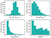 |
Fig. 1. Distribution of the main physical properties of interest in the whole sample. SFRs and stellar masses are corrected for magnification. |
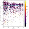 |
Fig. 2. Distance from the main sequence Δ(MS) = log(SFRMS)−log(SFR) (from Speagle et al. 2014) as a function of redshift for the galaxies in the full sample. The points are color-coded according to stellar mass. The dashed line at Δ(MS) = − 0.5 highlights the region from which quiescent galaxies were excluded (see the appendix, which is available on Zenodo). |
To further evaluate the completeness and reliability of the sample, we compared its stellar mass function (SMF) to the function derived in the COSMOS2020 sample (Weaver et al. 2023, 2022). To derive the SMF of our sample, we counted the number of galaxies in a given redshift bin separately for each cluster and divided it by the corresponding volume, corrected for the mean magnification of the sources in the studied bin. The comparison is shown in Figure 3. The studied sample seems to present an overdensity of sources at z > 4 and underestimates sources in the 2 < z ≤ 3 bin, especially at high masses. This might be due to the misidentification of low-redshift as high-redshift sources, as was also discussed in Guerrero et al. (2023). Kokorev et al. (2022) compared the spectroscopic redshifts for ∼7000 galaxies to the photometric redshifts they derived. While ∼80% of the redshifts agreed reasonably well, the remaining ∼20% presented large to sometimes catastrophic (Δz > 3) errors, mainly due to the confusion of the Lyman, Balmer, and 4000 Å breaks. In addition, an underevaluation of the survey volume (from an overevaluation of the corresponding magnification) might also artificially boost the source density. The potential impact of the derived SMF is further discussed in Sect. 5.
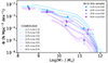 |
Fig. 3. Comparison between the SMF of the COSMOS2020 sample (Weaver et al. 2023, 2022) and the SMF of the sources studied in this paper. The SMF was obtained by counting the galaxies in each redshift bin separately for each cluster and dividing by the corresponding volume, corrected for the mean magnification of the sources in each bin. The error bars correspond to the 16th to 84th percentile of the stellar mass of the sources in the sample, and the impact of the 20% error on the magnification on the total volume. |
2.3. Subsamples
To study the evolution of the dust mass across redshift, we separated the sources into four redshift bins: 1 ≤ z < 2, 2 ≤ z < 3, 3 ≤ z < 4, and 4 ≤ z < 5. We additionally split sources according to either their SFRs or stellar masses into the following bins: (i) SFR (upper and lower limits in M⊙ yr−1): 0.001≤ SFR ≤1, 1< SFR ≤10, 10< SFR ≤50, 50< SFR ≤100, and 100< SFR ≤1000, and (ii) stellar mass (M*, upper and lower limits in M⊙): 108 ≤ M* ≤ 109, 109 < M* ≤ 1010, 1010 < M* ≤ 1011, and 1011 < M* ≤ 1012. The total number of sources in each subsample is listed in Table 2. Furthermore, the distribution of the SFR and stellar mass in each subsample can be found in the appendix (available on Zenodo).
Number of stacked sources in each subsample.
Sources that were individually detected in the ALCS data were not excluded from the samples. We decided to distinguish solely based on the properties mentioned above to derive the average properties of the population, and the 1.2 mm continuum flux density of individual sources should therefore not be a criterion of exclusion from our samples. To assess the impact of the 1.2 mm flux distribution in our samples, we performed median stacking and bootstrapping analyses, alongside the main mean-stacking analyses (see Sects. 3.4 and 4.2).
3. Methods
3.1. Stacking
We performed the stacking with LINESTACKER (Jolly et al. 2020) in single-channel mode (for the continuum stacking) on uv-tapered images (see Sect. 2.1). Sources were stacked pixel to pixel using mean stacks without weights (median stacks were also performed; see Section 4.2). The stacking was operated with stamp sizes of 9.76 × 9.76 arcsec2 (61 × 61 pixels). The sources were spatially aligned using the position extracted from the Kokorev et al. (2022) catalog. The stacked flux in Jy was retrieved by integrating the continuum flux in a central circular region of the stack stamp, with a radius Rinteg = 2″ (12.5 pixels). This corresponds to the synthesized beam size. We then divided it by the beam size in pixel units.
To compute the RMS associated with each stacked cube, a random set of source-free coordinates was drawn for each stacking position. An empty stack was then generated from the set of random coordinates (see Jolly et al. 2020) with the same characteristics as the normal stacks (i.e., stamp size and number of targets). This process was performed 1000 times for each subsample. The standard deviation across all stack stamps was then computed and used to derive the RMS associated with each stack cube. When the flux in the central region of the stack stamp was lower than three times its associated RMS, an upper limit of 3σ was used in place of the integrated flux to compute Mdust.
3.2. Magnification corrections
The averaged 1.2 mm fluxes extracted from each stack maps were corrected for the mean magnification of the sources in the stack subsample. The final flux was therefore computed as  , where Ffinal is the final flux we used to compute the dust mass (see Sect. 3.3), Fstack is the flux obtained from the stacked map, and
  is the average magnification of each source in the subsample. Alternatively, each source could be corrected for its magnification before stacking, Ffinal = Fcorrected stack, where Fcorrected stack is the flux obtained from the stack of the individually magnification-corrected maps,
  , where Mapstack is the stacked map obtained from individually magnification-corrected stamps (from which Fcorrected stack is obtained), n is the number of sources in the subsample, Stampi is the map-stamp associated with source i, and μi is the magnification associated with source i. We decided to correct for the average magnification of the sample after stacking because the signal in each stack stamp consists of the flux from the source, which is gravitationally magnified, and some noise, which is independent of the magnification. By correcting each stack stamp for its associated magnification, we corrected the flux from the source and the foreground noise. The efficiency of stacking is based on the fact that the noise is random and approximately similar in every stack stamp. By downscaling the noise in each stamp by a different number (unrelated to the noise properties), we might effectively reduce the efficiency and reliability of the stacking analysis. However, by correcting the final stack with the average magnification, the analysis would be biased toward high-magnification sources. Correcting each stamp individually pre-stacking should avoid this bias, and we therefore repeated our analysis with this correction method. The 1.2 mm fluxes derived in both cases are very consistent, and the values overlap within the error margins.
3.3. Measuring Mdust
To derive dust masses using the 1.2 mm continuum flux extracted from each stacking stamp, we used a single modified blackbody curve under the approximation of an optically thin regime. Following Kovács et al. (2010) and Magnelli et al. (2020), we defined Mdust as
where Mdust is the dust mass in M⊙, Sνobs is the flux at the observed frequency in Jy (and corrected for the average magnification, as explained in Sect. 3.2), νobs = νrest/(1 + z) is the observed frequency, fCMB is the correction factor to account for the cosmic microwave background (CMB; see details further in the text), DL is the luminosity distance in meter at redshift z, Bνobs(Tobs) is Planck’s blackbody function in Jy sr−1 at the observed temperature Tobs (Tobs = Trest/(1 + z)), κν0 is the photon cross section to mass ratio of dust in m2 kg−1, and β is the dust emissivity index. Sνobs was obtained by integrating over a fixed circular region in the center of the stack stamp (see Section 3.1).
Following Magnelli et al. (2020) and Pozzi et al. (2021), we decided to use a single cold component to account for the dust temperature, and we used a mass-weighted dust temperature of Trest = 25 K. While the total dust in galaxies is thought to consist of a warmer (20 < T < 60 K) and a colder (T < 30 K) component, studies of local galaxies have shown that the cold component causes most of the dust budget (from 96% to 99%, see Orellana et al. 2017) and the majority of the Rayleigh-Jeans emission (see also Shivaei et al. 2022, for a study of the contribution of the cold and warm dust components to the dust continuum emission at z ∼ 2). Scoville et al. (2014, 2016, 2017) argued that this approximation is probably still valid in higher-redshift galaxies. We decided to adopt Trest = 25 K at all redshifts probed by our analyses, but we note that dust masses evolve as T−1, meaning that our dust-mass results are effectively highly dependent on the estimated dust temperature, and that the masses derived in our analyses might be off by factors of a few if the assumed dust temperature is not correct (see Sect. 5).
While it might seem more appropriate to choose a dust temperature that evolves with redshift, we decided to maintain a fixed value to facilitate the comparison with similar previous studies. We used β = 1.8, the Galactic dust emissivity index measurement from the Planck data (Planck Collaboration XXI 2011), which also correlates well with values observed in high-redshift galaxies (e.g. Chapin et al. 2009; Magnelli et al. 2012; Faisst et al. 2020). Theoretical studies predicted values for β that range from 1.5 to 2.0 (e.g. Draine 2011), and similarly, observational studies such as Faisst et al. (2020) reported β values between 1.6 and 2.4 (with a median value of 2.0). The effect of β is weaker than the choice of the dust temperature, however, and we found that choosing β = 1.5 (or 2.0) would only modify our results by ∼9% at z = 1.5 and ∼15% at z = 5.5. We used κν0 = 0.0431 m2 kg−1 with ν0 = 352.6 GHz (Li & Draine 2001; Magnelli et al. 2020). We refer to Sect. 5 for a more complete discussion of the choice of parameters for the dust-mass computation.
Following da Cunha et al. (2013), we corrected our flux measurements for the effect of the CMB. First, we corrected our dust temperature for the additional heating through the CMB (following Equation (12) of da Cunha et al. 2013). This effect is minor because the dust temperature is only increased by ∼3% at z = 6 (the effect being even less important at lower redshift). Second, and most importantly, the CMB acts as a bright observing background, leading to an underestimation of the total flux. This was corrected for by following Equation (18) of da Cunha et al. (2013). This effect is much more important, as it yields an upward measurement to our results that ranges from ∼1.03 at z ∼ 1 to ∼1.31 at z ∼ 6.
3.4. Computing the uncertainty
To compute the overall uncertainties associated with our measurements, we combined different sources of uncertainties. The first source was the direct RMS from each stack analysis (computed from source-free stacks of each subsample; see Sect. 3.1). In addition,the intrinsic flux distribution of the sources in the sample needs to be accounted for in stacking analyses. To do this, we performed a bootstrapping analysis for each subsample. In each subsample, the dust mass was recomputed 1000 times, each time with a different sample, randomized from the original subsample without replacement (see Jolly et al. (2020) for a detailed description of the bootstrapping routine included in LINESTACKER). The distribution of the dust masses computed in this manner is shown in the appendix (available on Zenodo), where we also show the dust mass obtained from the original subsample (vertical black line). The peaks and shapes of the distributions are overall consistent with the values derived from the original samples. However, the peak of the distributions in most of the subsamples is slightly lower than in the original stacks. Similarly, some distributions present a faint tail toward higher dust masses. These two pieces of information combined indicate a skewed distribution, which can easily be explained because the samples contain individual detections. These effects are small, however, and should be well represented by the associated uncertainties on the dust-mass measurements.
From the distributions derived from of each bootstrapping analyses, we extracted the 16th to 84th percentile (see the appendix available on Zenodo), which we summed quadratically with the stack RMS1. In addition, because the redshift is used multiple times in equation 1, its 16th to 84th percentile in each subsample was used to propagate the associated uncertainty on the dust-mass computation. Finally, following Sun et al. (2022) and Fujimoto et al. (2023), we used a magnification uncertainty of 20% of the magnification associated with each subsample, and we propagated it to the aforementioned errors.
The 16th and 84th percentile of the (magnification-corrected) SFRs and stellar masses in each subsample were used to compute the error associated with the SFRs and stellar masses.
The combination of these measurement uncertainties was used to plot the error bars in the different figures shown in this work. However, only the RMS associated with each cube was used to qualify a detection or an upper limit (as stated in Sect. 3.1).
4. Results
4.1. Mean stacking results and dust continuum detection
The standard deviation in stack stamps reaches levels as low as ∼4.3 × 10⁻³ mJy per beam in the z = 1 − 2 bin of the lowest stellar mass and SFR subsamples (both containing ∼1000 sources). The total flux in the central circular aperture with a radius of 2 arcsec varies between ∼1.78 × 10⁻² mJy and ∼1.04 mJy for stack detections (flux above 3σ, not corrected for magnification). Securely extracted dust masses (with an S/N above 3σ) range from ∼2.8 × 10⁶ M⊙ to ∼2.56 × 10⁸ M⊙ (after correction for magnification). Figure 4 shows the stacked maps we obtained for each of the subsamples, from which we extracted the results presented below.
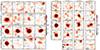 |
Fig. 4. 1.2 mm continuum stack maps. (left panel) 9.76 × 9.76 arcsec2 (61 × 61 pixels) mean stacking stamps, split into bins of stellar mass and redshift. Each map is normalized by the corresponding standard deviation, computed in associated empty stacks (see Sect. 3.1). The number of sources stacked (N) is indicated for each bin. (right panel) Similar to the left panel, but using SFR bins instead of stellar mass ones. |
The evolution of the dust mass with stellar mass and redshift is shown in Figure 5 and tabulated in Table 3. While detections in the lowest-redshift bin (1 < z < 2) indicate a clear linear relation between log(Mdust) and log(M*), the other redshift bins are less regular (see the left panel of Figure 5). When compared to other works (Santini et al. 2014; da Cunha et al. 2015; Kirkpatrick et al. 2017; Shivaei et al. 2022, also plotted on the figures), our data points are typically below other measurements (individual detections and stacks). This behavior is strongly reduced when quiescent galaxies are excluded from the stacks, however (see the appendix, which is available on Zenodo). This highlights that quiescent galaxies might have lower dust masses at the same stellar mass.
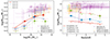 |
Fig. 5. Average dust mass evolution with stellar mass and redshift. (left) Average dust mass as a function of the stellar mass in each redshift bin. The circles represent detections (above 3σ), and down-pointing arrows represent 3σ upper limits. The error bars on the dust-mass detections were computed using a combination of different errors (see Sect. 3.4). The error bar along the x-axis represents the 16th to 84th percentile of parameter distribution in the stacked sample. (right) Similar to the left panel, but plotted as a function of redshift in each stellar mass bin. We also show for comparison individual dust-mass measurements detections (da Cunha et al. 2015; Kirkpatrick et al. 2017) and stacking measurements from Santini et al. (2014), Shivaei et al. (2022). |
Stacking results in the stellar mass subsamples.
The log(Mdust) – log(SFR) relation seems to follow a similar trend of increasing dust mass with increasing SFR, but with a clearer linear relation across redshift (although there is a higher number of nondetections; see the left panel of Figure 6 and the stacking results tabulated in Table 4), which indicates that the SFR might be better suited than the stellar mass to trace the dust mass. When compared to previous works (Santini et al. 2014; da Cunha et al. 2015; Kirkpatrick et al. 2017; Shivaei et al. 2022), our measurements follow a similar trend as was already observed, but they reach so far mostly unexplored regimes.
The evolution of the dust mass with redshift (see the right panels of Figures 5 and 6 and Figure 7) shows a relatively clear linear trend that indicates a decrease in the dust mass with increasing redshift.
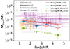 |
Fig. 7. Ratio of the average dust mass to average stellar mass as a function of redshift. Similar to the right panel of Figure 5, but normalized by the stellar mass of the galaxies in the sample. The error bars combine the error on the dust-mass computation and stellar mass distribution. |
By fitting quadratic functions to the data shown in Figures 5 and 6, we derived scaling relations between Mdust and M* at fixed z; Mdust and z at fixed M*; Mdust and SFR at fixed z; and Mdust and z at fixed SFR. The fits were performed using detections only (ignoring upper limits), and only when the number of data points was ≥3. The results from the fits are summarized in Table 5, and they are plotted in the appendix (available on Zenodo).
Fitting results.
4.2. Median stacking analysis
To better assess the effect of the population distribution on the derived dust mass, we also performed median stacks in the same way as the average stacks presented in Sect. 3.1. The overall median dust masses derived through our stacking analyses are systematically slightly lower than the mean dust masses (see Figure 8 for an illustration and the appendix available on Zenodo for detailed plots). While the median stellar mass and SFR of each subsample are also systematically lower than the mean (see the figures in the appendix), the difference is not large enough to explain the offset dust mass observed between the mean and median stacks. This again indicates a possibly skewed distribution of the dust mass in each subsample that results in offsets between the mean and median dust masses. However, we note that the dust-mass trends observed in this analysis (with redshift, stellar mass, and SFR) remain the same in the median stacking analyses.
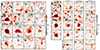 |
Fig. 8. Median stacking stamps, split into stellar mass and redshift (left panel) and SFR and redshift (right panel). Similar to Figure 4. |
5. Discussion
As our analysis focused on galaxies spanning a wide redshift range and our observation remained at a fixed observed wavelength, it is important to question the assumption made here that the continuum flux traces the same physical process at a rest wavelength λrest ∼ 0.5 mm (corresponding to z ∼ 1) and λrest ∼ 0.18 mm (corresponding to z ∼ 5). More specifically, the validity of the dust-mass equation (see Sect. 3.3) comes from the assumption that the dust is optically thin and that the flux measurement probes the Rayleigh-Jeans dust emission. This means that the part of the SED that is dominated by the emission of the dust at T = 25 K dominates the dust-mass budget. This is true at long wavelengths, where we effectively probe the Rayleigh-Jeans tail of the dust emission (e.g. Magdis et al. 2012; Scoville et al. 2016). However, the higher the redshift observed, the closer the region to the peak of the dust emission, which is more sensitive to temperature and total luminosity. This might explain the low detection rate in the high-z subsamples, even when the number of stack sources is high, and for which the corresponding RMS in the stack maps is low.
While numerous studies showed an evolution of the dust temperature with redshift, it is important to distinguish between the peak temperature, which is thought from theoretical and observational works to increase with redshift (e.g. Magdis et al. 2012; Magnelli et al. 2014; Béthermin et al. 2015; Ferrara et al. 2017; Narayanan et al. 2018; Schreiber et al. 2018; Liang et al. 2019; Ma et al. 2019; Sommovigo et al. 2020), and the mass-weighted temperature that probes the Rayleigh-Jeans tail, which can be directly used to measure the dust mass, as stated above. Unlike the peak temperature, the mass-weighted temperature is thought to be mostly constant with redshift (see Scoville et al. 2016; Liang et al. 2019). It should be noted, however, that the mass-weighted temperature still exhibits a small range in possible values, typically from 15 to 45 K (e.g. Liang et al. 2019), and a small increase with redshift may exist. On the other hand, Dudzevičiūtė et al. (2020) argued that the previously observed evolution of the dust temperature is likely due to the luminosity evolution in the samples employed, and they suggested a dust temperature of 30.4 ± 0.3, constant with redshift. In any event, to facilitate comparison with studies similar to ours and to limit complexity, we decided to keep a fixed temperature at all redshifts for the dust-mass computations. Consequently, for a T = 40 K (instead of 25) in the dust-mass computation, our results would change by ∼50% in the highest-redshift bin.
When comparing our results to the semi-analytical modeling from Popping et al. (2017), Lagos et al. (2019), Vijayan et al. (2019), Triani et al. (2020, see Figures 9 and 10)2 we can see an overall decent agreement in dust-mass predictions as a function of stellar mass at z ∼ 1. However, all models but the one presented in Vijayan et al. (2019) predict an overall increase in the dust mass with redshift while our analysis shows the opposite. In addition, the dust mass derived in the high-mass end of our subsamples is typically lower than predicted by the models (although this flattening might be due to the presence of quiescent galaxies in our sample, as shown in the appendix available on Zenodo). In addition, the method that is used to compute the average dust mass in the SHARK model (Lagos et al. 2019) differs from the one used in this work. To highlight this difference, we show in Figures 9 and 10 the average dust masses predicted by the SHARK model and the dust masses computed using equation 1 from the band 6 continuum (S6) predicted by SHARK. It is interesting to note that at z ∼ 3 and at z ∼ 5, the dust mass derived using the predicted S6 differs by almost one dex from the dust mass predicted otherwise. As mentioned above, this might be a direct consequence of the evolution of the rest wavelength with redshift, which moves the observation closer to the peak of the dust emission. Surprisingly, however, our results seem to agree better with the direct dust-mass measurements compared to those obtained from S6.
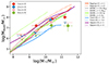 |
Fig. 9. Log average dust mass recovered as a function of the (log) stellar mass in each redshift bin. The circles represent detections (above 3σ), and the 3σ upper limits are represented by down-pointing arrows. We overplot the z = 1 and z = 6 dust mass-stellar mass relation from Popping et al. (2017) and the z ∼ 1 and z ∼ 5 relations from Lagos et al. (2019) (SHARK model), Triani et al. (2020), and Vijayan et al. (2019). We show the average dust mass directly predicted by the SHARK model and the dust mass computed from the predicted band 6 flux following Eq. (1). |
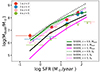 |
Fig. 10. Similar to Figure 9, but for the SFR instead of the stellar mass. The predictions from Lagos et al. (2019, SHARK model) at z ∼ 1, 3, and 5 are shown in terms of direct dust-mass predictions and dust mass inferred from predicted band 6 flux, following Eq. (1). |
As the analysis relies on photometric redshifts for a large fraction of the catalog, it is important to consider the potential impact this might have on the results. In particular, we note that the bins at z > 3 appear to be overpopulated. This is shown in Figure 3, where we compare the SMF of our sample to the SMF of the COSMOS2020 sample (Weaver et al. 2023, 2022). As a consequence, the dust content at z > 3 is likely overestimated. This is probably due to the misclassification of some lower-redshift sources to higher redshift, as suggested in Kokorev et al. (2022) and mentioned in Sect. 2.2.
Moreover, because the catalog we used was generated using HST and Spitzer photometry, some of the most dusty galaxies may be missing. This biases the analysis toward lower averaged dust masses. As pointed out in Kokorev et al. (2022), only 145 of the 180 sources that were individually detected with an S/N > 4 in the ALCS data are identified in their catalog. This indicates that some of the most dusty galaxies may be missing from our analysis. This bias could be strongest in the high-redshift bins, where only the UV-brightest galaxies (i.e., typically less obscured by dust) might be observed. The use of catalogs based on data from the James Webb Space Telescope (JWST) might help us to include more of the missing dusty galaxies, especially at high z, and to improve the SED-fitting routines.
As shown in the appendix (available on Zenodo), the inclusion of quiescent galaxies in the stacks biases the analysis toward lower dust masses, especially in the samples that are split according to stellar mass. This highlights that some sources that are included in the high-mass subsamples have a low SFR and also low dust masses. The higher average dust mass observed in the mass-selected samples without sources with ΔMS < −0.5 and the relatively stable average dust mass in SFR-selected samples implies that the SFR probably is a better dust-mass tracer. It shows in addition that quiescent galaxies typically have a lower dust content than their star-forming counterparts at similar stellar mass.
As in Magnelli et al. (2020), we used the dust opacities from Li & Draine (2001) to derive the dust masses. These values were constrained from observations of the diffuse interstellar medium (ISM), and these properties are therefore representative of dust in the diffuse ISM. However, some studies in nearby galaxies (e.g. Galliano et al. 2018) showed that the opacity from Li & Draine (2001) might have been underestimated by a factor of 2 − 3. Higher opacity values in galaxies do not mean that the values of Li & Draine (2001) are incorrect. Their values were constrained for the diffuse interstellar medium and are therefore well adapted for galaxies only if the bulk of the dust emission emerges from the diffuse interstellar medium of galaxies. The underestimation of the dust opacity might indicate that the majority of the dust emission does not emerge from diffuse regions, but from denser regions in which dust grains are likely to be larger.
In dense regions of the ISM, dust grains grow through accretion and coagulation, which triggers an increase in the dust opacity by a factor 2 − 3 (e.g. Köhler et al. 2015). The underestimation of the dust opacities in some nearby galaxies might therefore mean that the bulk of the dust emission arises from dense regions in which dust grains are larger than in the diffuse ISM. This seems to be the case in high-redshift galaxies as well, as Magnelli et al. (2020) claimed that the bulk of the dust emission in their galaxy sample emerged from the molecular phase, and therefore, from dense regions in which dust differs from the diffuse ISM. They also stated that there might be a significant increase in the dust emissivity from diffuse to denser regions, which can be explained in terms of grain growth (e.g. Köhler et al. 2015).
There is currently no consensus on the dust properties that must be considered in nearby or in high-redshift galaxies. Moreover, dust grains are probably not the same within galaxies and from one galaxy to the next, which adds to the complexity. Although diffuse ISM-like dust grains might not cause the majority of the dust emission in galaxies, these dust models have the advantage of being thoroughly developed and extensively used. We therefore use these dust properties from the diffuse ISM until we have more constraints on the dust grains that cause the emission in these galaxies.
6. Summary
We used deep ALMA band 6 data over 33 lensing clusters to perform a set of stacking analyses on a large sample of 4103 lensed sources, whose positions and physical parameters were extracted from the HST/IRAC catalog presented in Kokorev et al. (2022). The sample spanned redshifts from z = 1 to z = 5, SFRs from 0.001 M⊙ yr−1 to 1000 M⊙ yr−1, and stellar masses from 108 M⊙ to 1012 M⊙. To study the evolution of the dust mass through cosmic time, we binned the sources into five different redshifts bins, and we also grouped sources according to their SFR and stellar mass. We performed a continuum stacking on each of the subsamples using LINESTACKER (Jolly et al. 2020).
Using the mean continuum-stacked flux, we computed average dust masses. From the nondetections, we derived 3σ upper limits. Using detections and upper limits, we studied the evolution trend of the dust mass with redshift. We found clear indications for an average decrease in the dust mass with redshift. Similarly, we studied the evolution of the dust mass with stellar mass and SFR. In both cases, we found a positive correlation. From our detections, we derived the relations between the dust mass and SFR or stellar mass in different redshift ranges. The results from our study are mostly consistent with the results from modeling (at least at z ∼ 1) and from other similar studies. Our analysis allowed us to probe regimes of the stellar mass and SFR that were unexplored so far. The highest-redshift bin shows mostly nondetections, and the corresponding upper limits indicate low average dust masses (even though the overall RMS is low) when compared to other studies. This could be due to the different rest-wavelength probed at high z, lying closer to the peak of the dust emission. Alternatively, the reason might be the tendency of individual high-z dust measurements to be biased toward very dust-bright objects.
The linear trends observed between stellar mass and dust mass confirm that as galaxies evolve and form more stars, they also accumulate more dust. These dust grains play a vital role in catalyzing the formation of H2. In this way, they affect the overall gas reservoir that is available for future star formation. Dust becomes an integral component of a self-perpetuating cycle, accumulating throughout the stellar life cycle and subsequently bolstering the SFR. In addition, the inverse trend observed between the average dust mass and redshift implies that the buildup of dust in galaxies over cosmic time is a gradual process that is aligned with the overall evolution of the SFR density (e.g. Magnelli et al. 2020). This further indicates a gradual increase in the average metallicity in galaxies with cosmic time, as dust grains are known to be composed of heavy elements that are produced in stars.
Data availability
Appendices are available on https://zenodo.org/records/14224076
The SHARK model (Lagos et al. 2019) does not directly track the buildup and destruction of dust. Instead, dust masses are estimated assuming an empirical z = 0 relation between the dust-to-gas ratio and gas-phase metallicity.
Acknowledgments
The authors thank the anonymous reviewer for their thoughtful and constructive suggestions, which greatly helped improve this manuscript. This paper makes use of the ALMA data: ALMA #2018.1.00035.L, #2013.1.00999.S, and #2015.1.01425.S. ALMA is a partnership of the ESO (representing its member states), NSF (USA) and NINS (Japan), together with NRC (Canada), MOST and ASIAA (Taiwan), and KASI (Republic of Korea), in cooperation with the Republic of Chile. The Joint ALMA Observatory is operated by the ESO, AUI/NRAO, and NAOJ. JBJ thanks Ian Smail for the discussion. KK acknowledges support from the Swedish Research Council (2015-05580), and the Knut and Alice Wallenberg Foundation (KAW 2020.0081). K. Kohno acknowledges the JSPS KAKENHI Grant Numbers JP17H06130, JP22H04939, JP23K20035, JP24H00004, and the NAOJ ALMA Scientific Research Grant Number 2017-06B. AG acknowledges funding from ANID-Chile NCN2023_002 and FONDECYT Regular 1171506. DE acknowledges support from a Beatriz Galindo senior fellowship (BG20/00224) from the Spanish Ministry of Science and Innovation, projects PID2020-114414GB-100 and PID2020-113689GB-I00 financed by MCIN/AEI/10.13039/501100011033, project P20_00334 financed by the Junta de Andalucía, project A-FQM-510-UGR20 of the FEDER/Junta de Andalucía-Consejería de Transformación Económica, Industria, Conocimiento y Universidades. FEB acknowledges support from ANID-Chile BASAL CATA FB210003, FONDECYT Regular 1200495 and 1190818, and Millennium Science Initiative Program – ICN12_009.
References
- Aravena, M., Boogaard, L., Gónzalez-López, J., et al. 2020, ApJ, 901, 79 [NASA ADS] [CrossRef] [Google Scholar]
- Bertoldi, F., Carilli, C. L., Cox, P., et al. 2003, A&A, 406, L55 [NASA ADS] [CrossRef] [EDP Sciences] [Google Scholar]
- Béthermin, M., Daddi, E., Magdis, G., et al. 2015, A&A, 573, A113 [Google Scholar]
- Béthermin, M., Fudamoto, Y., Ginolfi, M., et al. 2020, A&A, 643, A2 [Google Scholar]
- Birkin, J. E., Weiss, A., Wardlow, J. L., et al. 2021, MNRAS, 501, 3926 [Google Scholar]
- Bouwens, R., González-López, J., Aravena, M., et al. 2020, ApJ, 902, 112 [NASA ADS] [CrossRef] [Google Scholar]
- Casey, C. M. 2012, MNRAS, 425, 3094 [Google Scholar]
- Casey, C. M., Narayanan, D., & Cooray, A. 2014, Phys. Rep., 541, 45 [Google Scholar]
- Chapin, E. L., Pope, A., Scott, D., et al. 2009, MNRAS, 398, 1793 [NASA ADS] [CrossRef] [Google Scholar]
- Coe, D., Salmon, B., Bradač, M., et al. 2019, ApJ, 884, 85 [Google Scholar]
- Combes, F. 2018, A&ARv, 26, 5 [NASA ADS] [CrossRef] [Google Scholar]
- da Cunha, E., Eminian, C., Charlot, S., & Blaizot, J. 2010, MNRAS, 403, 1894 [Google Scholar]
- da Cunha, E., Groves, B., Walter, F., et al. 2013, ApJ, 766, 13 [Google Scholar]
- da Cunha, E., Walter, F., Smail, I. R., et al. 2015, ApJ, 806, 110 [Google Scholar]
- Draine, B. T. 2011, Physics of the Interstellar and Intergalactic Medium (Princeton University Press) [Google Scholar]
- Draine, B. T., Dale, D. A., Bendo, G., et al. 2007, ApJ, 663, 866 [NASA ADS] [CrossRef] [Google Scholar]
- Driver, S. P., Andrews, S. K., da Cunha, E., et al. 2018, MNRAS, 475, 2891 [Google Scholar]
- Dudzevičiūtė, U., Smail, I., Swinbank, A. M., et al. 2020, MNRAS, 494, 3828 [Google Scholar]
- Dudzevičiūtė, U., Smail, I., Swinbank, A. M., et al. 2021, MNRAS, 500, 942 [Google Scholar]
- Engelbracht, C. W., Rieke, G. H., Gordon, K. D., et al. 2008, ApJ, 678, 804 [NASA ADS] [CrossRef] [Google Scholar]
- Faisst, A. L., Fudamoto, Y., Oesch, P. A., et al. 2020, MNRAS, 498, 4192 [NASA ADS] [CrossRef] [Google Scholar]
- Ferrara, A., Hirashita, H., Ouchi, M., & Fujimoto, S. 2017, MNRAS, 471, 5018 [NASA ADS] [CrossRef] [Google Scholar]
- Fujimoto, S., Kohno, K., Ouchi, M., et al. 2023, arXiv e-prints [arXiv:2303.01658] [Google Scholar]
- Galametz, M., Madden, S. C., Galliano, F., et al. 2011, A&A, 532, A56 [NASA ADS] [CrossRef] [EDP Sciences] [Google Scholar]
- Galliano, F., Galametz, M., & Jones, A. P. 2018, ARA&A, 56, 673 [Google Scholar]
- González-López, J., Bauer, F. E., Romero-Cañizales, C., et al. 2017, A&A, 597, A41 [NASA ADS] [CrossRef] [EDP Sciences] [Google Scholar]
- González-López, J., Novak, M., Decarli, R., et al. 2020, ApJ, 897, 91 [Google Scholar]
- Guerrero, A., Nagar, N., Kohno, K., et al. 2023, MNRAS, 526, 2423 [NASA ADS] [CrossRef] [Google Scholar]
- Hodge, J. A., & da Cunha, E. 2020, Roy. Soc. Open Sci., 7, 200556 [NASA ADS] [CrossRef] [Google Scholar]
- Hunt, L., Bianchi, S., & Maiolino, R. 2005, A&A, 434, 849 [NASA ADS] [CrossRef] [EDP Sciences] [Google Scholar]
- Jolly, J.-B., Knudsen, K. K., & Stanley, F. 2020, MNRAS, 499, 3992 [Google Scholar]
- Kirkpatrick, A., Pope, A., Sajina, A., et al. 2017, ApJ, 843, 71 [NASA ADS] [CrossRef] [Google Scholar]
- Knudsen, K. K., Richard, J., Kneib, J.-P., et al. 2016, MNRAS, 462, L6 [NASA ADS] [CrossRef] [Google Scholar]
- Köhler, M., Ysard, N., & Jones, A. P. 2015, A&A, 579, A15 [NASA ADS] [CrossRef] [EDP Sciences] [Google Scholar]
- Kohno, K., Fujimoto, S., Tsujita, A., et al. 2023, in Physics and Chemistry of Star Formation: The Dynamical ISM Across Time and Spatial Scales, eds. V. Ossenkopf-Okada, R. Schaaf, I. Breloy, & J. Stutzki, 16 [Google Scholar]
- Kokorev, V., Brammer, G., Fujimoto, S., et al. 2022, ApJS, 263, 38 [NASA ADS] [CrossRef] [Google Scholar]
- Kovács, A., Omont, A., Beelen, A., et al. 2010, ApJ, 717, 29 [CrossRef] [Google Scholar]
- Lagos, C. d. P., Robotham, A. S. G., Trayford, J. W., et al. 2019, MNRAS, 489, 4196 [NASA ADS] [CrossRef] [Google Scholar]
- Laporte, N., Ellis, R. S., Boone, F., et al. 2017, ApJ, 837, L21 [CrossRef] [Google Scholar]
- Li, A., & Draine, B. T. 2001, ApJ, 554, 778 [Google Scholar]
- Li, Q., Narayanan, D., & Davé, R. 2019, MNRAS, 490, 1425 [CrossRef] [Google Scholar]
- Liang, L., Feldmann, R., Kereš, D., et al. 2019, MNRAS, 489, 1397 [NASA ADS] [CrossRef] [Google Scholar]
- Lotz, J. M., Koekemoer, A., Coe, D., et al. 2017, ApJ, 837, 97 [Google Scholar]
- Ma, X., Hayward, C. C., Casey, C. M., et al. 2019, MNRAS, 487, 1844 [NASA ADS] [CrossRef] [Google Scholar]
- Magdis, G. E., Daddi, E., Béthermin, M., et al. 2012, ApJ, 760, 6 [NASA ADS] [CrossRef] [Google Scholar]
- Magnelli, B., Lutz, D., Santini, P., et al. 2012, A&A, 539, A155 [NASA ADS] [CrossRef] [EDP Sciences] [Google Scholar]
- Magnelli, B., Lutz, D., Saintonge, A., et al. 2014, A&A, 561, A86 [NASA ADS] [CrossRef] [EDP Sciences] [Google Scholar]
- Magnelli, B., Boogaard, L., Decarli, R., et al. 2020, ApJ, 892, 66 [NASA ADS] [CrossRef] [Google Scholar]
- Magrini, L., Bianchi, S., Corbelli, E., et al. 2011, A&A, 535, A13 [NASA ADS] [CrossRef] [EDP Sciences] [Google Scholar]
- McMullin, J. P., Waters, B., Schiebel, D., Young, W., & Golap, K. 2007, ASP Conf. Ser., 376, 127 [Google Scholar]
- Narayanan, D., Davé, R., Johnson, B. D., et al. 2018, MNRAS, 474, 1718 [NASA ADS] [CrossRef] [Google Scholar]
- Orellana, G., Nagar, N. M., Elbaz, D., et al. 2017, A&A, 602, A68 [NASA ADS] [CrossRef] [EDP Sciences] [Google Scholar]
- Planck Collaboration XXI. 2011, A&A, 536, A21 [NASA ADS] [CrossRef] [EDP Sciences] [Google Scholar]
- Popping, G., & Péroux, C. 2022, MNRAS, 513, 1531 [CrossRef] [Google Scholar]
- Popping, G., Somerville, R. S., & Galametz, M. 2017, MNRAS, 471, 3152 [NASA ADS] [CrossRef] [Google Scholar]
- Popping, G., Shivaei, I., Sanders, R. L., et al. 2023, A&A, 670, A138 [NASA ADS] [CrossRef] [EDP Sciences] [Google Scholar]
- Postman, M., Coe, D., Benítez, N., et al. 2012, ApJS, 199, 25 [Google Scholar]
- Pozzi, F., Calura, F., Zamorani, G., et al. 2020, MNRAS, 491, 5073 [NASA ADS] [CrossRef] [Google Scholar]
- Pozzi, F., Calura, F., Fudamoto, Y., et al. 2021, A&A, 653, A84 [NASA ADS] [CrossRef] [EDP Sciences] [Google Scholar]
- Rémy-Ruyer, A., Madden, S. C., Galliano, F., et al. 2014, A&A, 563, A31 [Google Scholar]
- Saintonge, A., Lutz, D., Genzel, R., et al. 2013, ApJ, 778, 2 [Google Scholar]
- Santini, P., Maiolino, R., Magnelli, B., et al. 2014, A&A, 562, A30 [NASA ADS] [CrossRef] [EDP Sciences] [Google Scholar]
- Schreiber, C., Glazebrook, K., Nanayakkara, T., et al. 2018, A&A, 618, A85 [NASA ADS] [CrossRef] [EDP Sciences] [Google Scholar]
- Scoville, N. Z. 2013, Evolution of star formation and gas, eds. J. Falcón-Barroso, & J. H. Knapen, 491 [Google Scholar]
- Scoville, N., Aussel, H., Sheth, K., et al. 2014, ApJ, 783, 84 [CrossRef] [Google Scholar]
- Scoville, N., Sheth, K., Aussel, H., et al. 2016, ApJ, 820, 83 [Google Scholar]
- Scoville, N., Lee, N., Vanden Bout, P., et al. 2017, ApJ, 837, 150 [Google Scholar]
- Shapley, A. E., Cullen, F., Dunlop, J. S., et al. 2020, ApJ, 903, L16 [NASA ADS] [CrossRef] [Google Scholar]
- Shivaei, I., Popping, G., Rieke, G., et al. 2022, ApJ, 928, 68 [NASA ADS] [CrossRef] [Google Scholar]
- Sommovigo, L., Ferrara, A., Pallottini, A., et al. 2020, MNRAS, 497, 956 [NASA ADS] [CrossRef] [Google Scholar]
- Speagle, J. S., Steinhardt, C. L., Capak, P. L., & Silverman, J. D. 2014, ApJS, 214, 15 [Google Scholar]
- Sun, F., Egami, E., Fujimoto, S., et al. 2022, ApJ, 932, 77 [CrossRef] [Google Scholar]
- Tacconi, L. J., Genzel, R., & Sternberg, A. 2020, ARA&A, 58, 157 [NASA ADS] [CrossRef] [Google Scholar]
- Tamura, Y., Mawatari, K., Hashimoto, T., et al. 2019, ApJ, 874, 27 [NASA ADS] [CrossRef] [Google Scholar]
- Tamura, Y. C., Bakx, T. J. L., Inoue, A. K., et al. 2023, ApJ, 952, 9 [NASA ADS] [CrossRef] [Google Scholar]
- Triani, D. P., Sinha, M., Croton, D. J., Pacifici, C., & Dwek, E. 2020, MNRAS, 493, 2490 [NASA ADS] [CrossRef] [Google Scholar]
- Valiante, R., Schneider, R., Bianchi, S., & Andersen, A. C. 2009, MNRAS, 397, 1661 [CrossRef] [Google Scholar]
- Venemans, B. P., McMahon, R. G., Walter, F., et al. 2012, ApJ, 751, L25 [NASA ADS] [CrossRef] [Google Scholar]
- Vijayan, A. P., Clay, S. J., Thomas, P. A., et al. 2019, MNRAS, 489, 4072 [NASA ADS] [CrossRef] [Google Scholar]
- Wakelam, V., Bron, E., Cazaux, S., et al. 2017, Mol. Astrophys., 9, 1 [Google Scholar]
- Walter, F., Decarli, R., Aravena, M., et al. 2016, ApJ, 833, 67 [Google Scholar]
- Watson, D., Christensen, L., Knudsen, K. K., et al. 2015, Nature, 519, 327 [Google Scholar]
- Weaver, J. R., Kauffmann, O. B., Ilbert, O., et al. 2022, ApJS, 258, 11 [NASA ADS] [CrossRef] [Google Scholar]
- Weaver, J. R., Davidzon, I., Toft, S., et al. 2023, A&A, 677, A184 [NASA ADS] [CrossRef] [EDP Sciences] [Google Scholar]
- Zavala, J. A., Casey, C. M., Manning, S. M., et al. 2021, ApJ, 909, 165 [CrossRef] [Google Scholar]
All Tables
All Figures
|
Fig. 1. Distribution of the main physical properties of interest in the whole sample. SFRs and stellar masses are corrected for magnification. |
| In the text | |
|
Fig. 2. Distance from the main sequence Δ(MS) = log(SFRMS)−log(SFR) (from Speagle et al. 2014) as a function of redshift for the galaxies in the full sample. The points are color-coded according to stellar mass. The dashed line at Δ(MS) = − 0.5 highlights the region from which quiescent galaxies were excluded (see the appendix, which is available on Zenodo). |
| In the text | |
|
Fig. 3. Comparison between the SMF of the COSMOS2020 sample (Weaver et al. 2023, 2022) and the SMF of the sources studied in this paper. The SMF was obtained by counting the galaxies in each redshift bin separately for each cluster and dividing by the corresponding volume, corrected for the mean magnification of the sources in each bin. The error bars correspond to the 16th to 84th percentile of the stellar mass of the sources in the sample, and the impact of the 20% error on the magnification on the total volume. |
| In the text | |
|
Fig. 4. 1.2 mm continuum stack maps. (left panel) 9.76 × 9.76 arcsec2 (61 × 61 pixels) mean stacking stamps, split into bins of stellar mass and redshift. Each map is normalized by the corresponding standard deviation, computed in associated empty stacks (see Sect. 3.1). The number of sources stacked (N) is indicated for each bin. (right panel) Similar to the left panel, but using SFR bins instead of stellar mass ones. |
| In the text | |
|
Fig. 5. Average dust mass evolution with stellar mass and redshift. (left) Average dust mass as a function of the stellar mass in each redshift bin. The circles represent detections (above 3σ), and down-pointing arrows represent 3σ upper limits. The error bars on the dust-mass detections were computed using a combination of different errors (see Sect. 3.4). The error bar along the x-axis represents the 16th to 84th percentile of parameter distribution in the stacked sample. (right) Similar to the left panel, but plotted as a function of redshift in each stellar mass bin. We also show for comparison individual dust-mass measurements detections (da Cunha et al. 2015; Kirkpatrick et al. 2017) and stacking measurements from Santini et al. (2014), Shivaei et al. (2022). |
| In the text | |
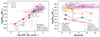 |
Fig. 6. Similar to Figure 5, but in SFR bins instead of stellar mass. |
| In the text | |
|
Fig. 7. Ratio of the average dust mass to average stellar mass as a function of redshift. Similar to the right panel of Figure 5, but normalized by the stellar mass of the galaxies in the sample. The error bars combine the error on the dust-mass computation and stellar mass distribution. |
| In the text | |
|
Fig. 8. Median stacking stamps, split into stellar mass and redshift (left panel) and SFR and redshift (right panel). Similar to Figure 4. |
| In the text | |
|
Fig. 9. Log average dust mass recovered as a function of the (log) stellar mass in each redshift bin. The circles represent detections (above 3σ), and the 3σ upper limits are represented by down-pointing arrows. We overplot the z = 1 and z = 6 dust mass-stellar mass relation from Popping et al. (2017) and the z ∼ 1 and z ∼ 5 relations from Lagos et al. (2019) (SHARK model), Triani et al. (2020), and Vijayan et al. (2019). We show the average dust mass directly predicted by the SHARK model and the dust mass computed from the predicted band 6 flux following Eq. (1). |
| In the text | |
|
Fig. 10. Similar to Figure 9, but for the SFR instead of the stellar mass. The predictions from Lagos et al. (2019, SHARK model) at z ∼ 1, 3, and 5 are shown in terms of direct dust-mass predictions and dust mass inferred from predicted band 6 flux, following Eq. (1). |
| In the text | |
Current usage metrics show cumulative count of Article Views (full-text article views including HTML views, PDF and ePub downloads, according to the available data) and Abstracts Views on Vision4Press platform.
Data correspond to usage on the plateform after 2015. The current usage metrics is available 48-96 hours after online publication and is updated daily on week days.
Initial download of the metrics may take a while.