| Issue |
A&A
Volume 692, December 2024
|
|
|---|---|---|
| Article Number | A203 | |
| Number of page(s) | 11 | |
| Section | Astrophysical processes | |
| DOI | https://doi.org/10.1051/0004-6361/202451773 | |
| Published online | 13 December 2024 | |
PKS 1424−418: A persistent candidate source of the mm–γ-ray connection?
1
Max-Planck-Institut für Radioastronomie, Auf dem Hügel 69, 53121 Bonn, Germany
2
Julius-Maximilians-Universität Würzburg, Fakultät für Physik und Astronomie, Institut für Theoretische Physik und Astrophysik, Lehrstuhl für Astronomie, Emil-Fischer-Str. 31, D-97074 Würzburg, Germany
⋆ Corresponding author; This email address is being protected from spambots. You need JavaScript enabled to view it.
Received:
2
August
2024
Accepted:
6
November
2024
Abstract
We present a long-term strong correlation between millimeter (mm) radio and γ-ray emission in the flat-spectrum radio quasar (FSRQ) PKS 1424−418. The mm–γ-ray connection in blazars is generally thought to originate from the relativistic jet close to the central engine. We confirm a unique long-lasting mm–γ-ray correlation of PKS 1424−418 by using detailed correlation analyses and statistical tests, and we find its physical meaning in the source. We employed ∼8.5 yr of (sub)mm and γ-ray light curves observed by ALMA and Fermi-LAT, respectively. From linear and cross-correlation analyses between the light curves, we found a significant, strong mm–γ-ray correlation over the whole period. We did not find any notable time delay within the uncertainties for the mm–γ-ray correlation, which means zero lag. The mm wave spectral index values (Sν ∝ να) between the bands 3 and 7 flux densities indicate a time-variable opacity of the source at (sub)mm wavelengths. Interestingly, the mm wave spectral index becomes temporarily flatter (i.e., α > −0.5) when the source flares in the γ-rays. We relate our results with the jet of PKS 1424−418, and we discuss the origin of the γ-rays and opacity of the inner (sub)parsec-scale jet regions.
Key words: radiation mechanisms: non-thermal / galaxies: active / galaxies: jets / gamma rays: galaxies / submillimeter: galaxies / quasars: individual: PKS 1424−418
© The Authors 2024
 Open Access article, published by EDP Sciences, under the terms of the Creative Commons Attribution License (https://creativecommons.org/licenses/by/4.0), which permits unrestricted use, distribution, and reproduction in any medium, provided the original work is properly cited.
This article is published in open access under the Subscribe to Open model.
Open access funding provided by Max Planck Society.
1. Introduction
Blazars are a subclass of radio-loud active galactic nuclei (AGNs). The vast majority of bright γ-ray sources detected by the Fermi-Large Area Telescope (LAT) are identified as AGNs (e.g., ≥80% reported in Ajello et al. 2020), and blazars dominate the γ-ray bright AGN population. Blazars can be further categorized into two subtypes: flat-spectrum radio quasars (FSRQs), and objects of BL Lacertae type (BLLacs). FSRQs show prominent optical emission lines, whereas BLLacs are without this feature (see also Keenan et al. 2021, for a recent study of the dichotomy on weak and strong jets). Blazars are strong nonthermal sources, and the typical spectral energy distribution (SED) of blazars consists of two hump-like features, one of which is indicative of the synchrotron process from the radio to the UV, and the other is often presumed to be the inverse-Compton (IC) process in the γ-ray regime. Alternatively, hadronic models have also been suggested for the γ-ray emission (e.g., Dar & Laor 1997; Böttcher 2007; Böttcher et al. 2013). X-ray bands can show a concave spectrum that is produced by both radiative processes (e.g., MAGIC Collaboration 2018). The relativistic jets in blazars are considered to be the main source of the nonthermal emissions, including in the γ-ray band (see e.g., Marscher et al. 2008, for a physical picture of the process). Due to the small viewing angles between the jet axis and the line of sight (e.g., typically ≤5°), emission from blazar jets is highly Doppler boosted and shows strong variability with time. An obvious question here is where and how the γ-rays are produced in the jets (Blandford et al. 2019).
With the development of very long-baseline interferometry (VLBI), detailed morphologies, structures, and physical properties of the (sub)parsec-scale jets of blazars were revealed (e.g., Lee et al. 2008; Lister et al. 2009; Nair et al. 2019; Weaver et al. 2022). In most of the VLBI images, the jets show a compact intense emitting region at the upstream end of the flow. This structure is called the radio core (or VLBI core), which is generally assumed to be the surface of the unity optical depth: τopaq(ν) ∼ 1. This leads to the so-called core shift in the jets and tends to decrease with increasing frequency in a power-law form (see e.g., Dodson et al. 2017). Hence, the innermost jet regions closer to the central engine are rather hidden and invisible owing to synchrotron self-absorption (SSA), particularly at lower radio frequencies (e.g., Lobanov 1998; Marscher et al. 2008; see also Marscher 2016 for alternative theories and models of the core). It has been suggested that the core shift is variable with time and can be increased by strong flares at higher radio frequencies (e.g., Chamani et al. 2023). In this context, observations at higher radio frequencies are crucial to broaden our understanding of the high-energy emission processes in blazar jets. Previous studies of the jets found that the γ-ray emission is correlated with the core radio emission (e.g., Jorstad et al. 2001a; Kovalev et al. 2009; Pushkarev et al. 2010, but see also Cheung et al. 2007; Hodgson et al. 2018, for the γ-rays with a different origin in the jets of some radio galaxies). Based on VLBI observations, it was suggested that the γ-ray events are tightly linked with the passage of superluminal knots through the radio core region (e.g., Jorstad et al. 2001b; Marscher et al. 2008; Wehrle et al. 2016; Röder et al. 2024).
The search for time correlations between radio and γ-ray light curves is one of the key approaches to support the existence of the radio–γ-ray connection in blazars. Previous studies performed a statistical study with a large number of AGN samples (mostly blazars) and found that just a handful of sources show a significant radio–γ-ray correlation over a short period (i.e., 2.5–5.0 yr) of time (Fuhrmann et al. 2014; Max-Moerbeck et al. 2014a; Ramakrishnan et al. 2015, 2016). In contrast to the clear correlation between the optical and γ-ray emission in blazars (e.g., Liodakis et al. 2019), it is difficult to find a clear significant correlation between radio and γ-ray emission. This might be due to (1) different variability timescales, (2) a lack of huge flares, and (3) poor data sampling. The typical radio–γ-ray correlation is either (1) the γ-rays preceding the radio emission (e.g., Agudo et al. 2011a; Kim et al. 2020) or (2) the γ-rays (quasi-)simultaneous with the radio emission (e.g., Wehrle et al. 2012; Kim et al. 2018). This suggests that the γ-ray production site is located either in a region upstream of or near the radio core (but see also León-Tavares et al. 2011, for a scenario of a region downstream from the core). In addition, previous and recent works reported multiple sites for γ-rays in the jets (e.g., Marscher et al. 2008; Rani et al. 2018; Liodakis et al. 2020; Kim et al. 2022).
PKS 1424−418 (z ∼ 1.52; White et al. 1988) is an FSRQ in the southern sky (Dec ∼ −42°). Since most of the major VLBI arrays are located in the northern hemisphere, there are only a limited number of VLBI images of this source. The jet of PKS 1424−418 has an extended structure toward the northeast in the image plane that indicates the flow axis (see Benke et al. 2024). Interestingly, a PeV-energy neutrino event was detected from this source along with strong γ-ray outbursts in late 2012 to early 2013 (Kadler et al. 2016). This implies the presence of hadronic processes (e.g., photo-pion production with highly accelerated protons) in the jet of PKS 1424−418.
In this work, we define the spectral index (α) as Sν ∝ να, where S and ν are the flux density and observing frequency, respectively. We estimated the uncertainty of α following the error propagation. We use the cosmological parameters as follows: H0 = 71 km Mpc s−1, ΩΛ = 0.73, and Ωm = 0.27 throughout this paper.
2. Radio and γ-ray light curves in 2011–2020
2.1. γ-ray data
We analyzed the Pass 8 γ-ray data obtained from the Fermi-LAT (Atwood et al. 2009). Overall, we followed the standard unbinned likelihood procedure1 to generate the γ-ray light curve of the source (i.e., RA = 216.987°, Dec = −42.106°; J2000). At first, we put together a background template (so-called XML model). Two background components, gll_iem_v07 and iso_P8R3_SOURCE_V3_v1, were employed to take into account Galactic diffuse emission and isotropic background emission, respectively. We set a region of interest (ROI) to be a circle of radius 10° centered at the position of PKS 1424−418, and we included all 4FGL-catalog sources (4FGL-DR4, Abdollahi et al. 2020; Ballet et al. 2023) present within 20° (ROI + 10°) from the position of PKS 1424−418. We kept the default spectral models provided by the catalog for all the sources except our target; a simple power law was applied to the target (see below).
During the spectral fits, we left the spectral parameters free for all sources within 5° of the ROI center. For sources between 5° and 10°, only normalization parameters were left free. For sources beyond 10°, we kept all the parameters fixed to the catalog values. For the two diffuse background components (i.e., Galactic and isotropic), only the normalizations were left free. When sources lay within 10° but were faint (i.e., < 5σ, where σ is the detection significance), then their spectral parameters were kept fixed; one source was known to be time variable (i.e., variability index > 24.73; see, e.g., Abdollahi et al. 2023 for a definition of the variability index), and thus, we only let its normalization be free.
We analyzed γ-rays from the source in the 0.1–200 GeV energy range measured between 4 September 2011 and 26 March 2020 (MJD: 55808–58934), which is ∼8.5 yr. We chose this time range because (1) the ALMA light curves of this source started in 2011 and (2) the source became quiescent in the LAT γ-ray band for a long time (i.e., ∼1.5 yr) with too many upper limits from 2020. We selected SOURCE class (evclass = 128) and FRONT+BACK-type (evtype = 3) events. The good-time intervals (GTIs) were determined with the parameters (DATA_QUAL>0)&&(LAT_CONFIG= = 1) and roicut=no. The maximum zenith angle (zmax) was set to be 90° to minimize the Earth limb γ-ray contamination. We employed the maximum likelihood test statistics (TS) to evaluate the significance of the γ-ray photons. For each time bin, we first fit the data with the background template. Then, all the faint sources with TS < 9 (∼3σ) were removed from the background model. Using this updated model, we performed a second maximum likelihood fit to the data to obtain the final results. We computed 2σ upper limits for the γ-rays with TS < 20 or ΔFγ/Fγ ≥ 0.5, where Fγ and ΔFγ indicate the γ-ray flux density and its uncertainty, respectively.
We used a power-law form that was defined as dN/dE ∝ EΓ, with N being the number of photons, E the photon energy, and Γ the photon index. For the LAT analysis, the power-law and LogParabola models2 are generally preferable for AGNs. In our case, there are no significant differences in the results between the two models, and we selected the power-law model assuming that it is more suitable for these short day-scale bins. Since we let Γ vary during the fits, every single time bin had a different Γ value. Figure 1 shows the results. Overall, Γ fluctuates in the time domain without a clear tendency. However, Γ seems to converge to about −2.0 with increasing flux density. The overall index–flux trend of PKS 1424−418 is similar to a typical pattern for γ-ray emitting FSRQs (see e.g., Kim et al. 2020, for the case of 3C 273), but fairly harder and brighter. To match the γ-ray data with the sampling of our radio data, we generated a γ-ray light curve with a binning interval of 6 days (see Section 2.2).
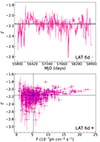 |
Fig. 1. Power-law index vs. time (upper) and flux density (lower) of the γ-ray emission of PKS 1424−418. The black lines in each panel indicate the median values on each axis: Γmedian = −2.17 and Fmedian = 5.39 × 10⁻⁷ ph cm−2 s−1. |
In total, we obtained 522 γ-ray photon measurements, including 14 bad time bins for which the fit was unsuccessful with some fitting errors. We excluded these poor data in this work. Only data points with TS ≥ 20 and ΔFγ/Fγ < 0.5 were used in this work, which is ∼93% (470/508) of the whole samples. For the other poor data points, we present the upper limits only in Figure 2, and they were excluded in the rest of our results. During the source analysis, we occasionally found that the fit returned erroneous results (e.g., empty or highly underestimated bins) depending on the fit-tolerance (Tol) value. To remedy this issue, we carried out two sets of the analysis: one set with Tol ∼ 0.01, and the other set with Tol ∼ 0.00001. When they both returned reasonable estimates, we chose the set with a higher TS or lower ΔFγ/Fγ when the difference in TS was smaller than one. In our γ-ray light curve, we defined the low-state photons as those with TS < 100 (76 photons in total). They are ∼3 × 10⁻⁷ ph cm−2 s−1 on average, with 1σ being ∼1.3 × 10⁻⁷ ph cm−2 s−1. Based on this estimate, we considered all those photons brighter than ∼7 × 10⁻⁷ ph cm−2 s−1 (i.e., ≥ the average +3σ) as a flare.
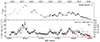 |
Fig. 2. ALMA band 3 (95 GHz) light curve (upper) and 6-day-binned LAT γ-ray light curve (lower) of PKS 1424−418 in 2011–2020 (∼8.5 yr). The red arrows indicate the 2σ upper limits of the γ-rays. The detection of γ-ray photons in terms of TS is shown as the light orange line. The horizontal blue line denotes the threshold for the γ-ray flare. |
2.2. Millimeter-wave data
We made use of the Atacama Large Millimeter/submillimeter Array (ALMA) calibrator catalog data3. We obtained three ALMA millimeter (mm) radio light curves of PKS 1424−418 at band 3, band 6, and band 7 (see more details of the ALMA bands here4). At band 3, the flux densities were measured at two central frequencies: ∼91 GHz and ∼103 GHz. We used all these measurements and consider 95 GHz as a representative observing frequency of band 3 in this study. When multiple flux density measurements were available at the same timestamp, we used their average. The other two bands (i.e., bands 6 and 7) observed the source at the central frequencies of ∼235 GHz and ∼345 GHz, respectively. Details of the catalog and ALMA observations can be found in Bonato et al. (2018).
In our analyses, the cadence (i.e., the sampling frequency) is the most important factor for obtaining more accurate results, and we found that the band 3 light curve was best sampled: The median sampling interval is 6 days, with an average of ∼10 days (see Appendix A for the bands 6 and 7 data). For all the ALMA bands, the medians describe their samplings better than the average (i.e., closer to the peak frequency in the sampling distribution). Since band 3 had a higher cadence than the other two radio bands, our analyses were more focused on the data from this band together with the LAT γ-ray data. As for the Fermi-LAT data analysis, we considered ALMA data spanning ∼8.5 yr from September 2011 to March 2020. Figure 2 shows the band 3 and γ-ray light curves. The band 3 flux densities are ∼3 Jansky (Jy) on average at 95 GHz with 1σ of 1 Jy. From simple visual inspection of the light curves, it seems already obvious that their overall patterns look very similar to each other, which implies a connection between the mm and γ-ray variability.
3. Results
While we estimated the median sampling times at the three ALMA bands, the radio light curves were sampled unevenly because the cadence varied, as shown in Figure 2. The γ-ray data, on the other hand, have some empty time bins (i.e., erroneous data) and upper limits that lead to irregular sampling. To properly account for this in our analyses, we developed a binning approach (see Appendix B), and this approach was used throughout this paper. A connection between the mm and γ-ray light curves was examined by using the Pearson correlation and the local cross-correlation function (LCCF; e.g., Welsh 1999). Detailed descriptions of these methods can be found in Appendix B and Appendix C, respectively.
3.1. Linear relations
The Pearson correlation is a straightforward way to examine the presence of any significant linear correlation between two time series. Figure 3 shows the results. We obtained a total of 488 Pearson coefficients (rP) for the whole 8.5 yr of the mm and γ-ray variability. Bineq (i.e., the equal-sized time bin) varies with the 488 calculations from 6–100 days. The rP values are ∼0.76 on average, with a 1σ uncertainty of 0.02 (minimum and maximum of 0.71 and 0.86, respectively). A sufficient number of data samples was used for each of the calculations, and thus, all the rP values are highly significant (i.e., p-values ≪ 0.01). As expected from the visual inspection of Figure 2, there is a clear and strong positive correlation between the band 3 and γ-ray emission in PKS 1424−418 in all observations. A level of rP = 0.76 is already quite high; even the minimum value of 0.71 is also high enough. Overall, the impact of different Bineq sizes on rP is shallow, but it is stronger above ∼30 days. This strong significant linear relation in the presence of multiple flaring activities at both wavebands for a long time indicates that the mm wave and γ-ray emissions are physically connected with each other (e.g., Wehrle et al. 2012). In Appendix A, we also test Pearson correlations between the three radio bands (i.e., bands 3, 6, and 7). As a result, we find that they are tightly correlated almost one to one with rP of > 0.95.
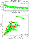 |
Fig. 3. Pearson correlation tests between the ALMA band 3 and LAT light curves for the whole 8.5 yr period. We estimated 488 different Pearson coefficients (rP) using different time-grids (see Appendix B). Upper panel: rP distribution on different scales of the time bin. The dashed red lines refer to the highest rP value (i.e., ∼0.86) at Bineq = 69.1 days (NBineq = 46). Lower panel: Flux–flux scatters corresponding to the rP estimates shown in the upper panel. The scatter for the highest rP is shown in red. The transparency of the data points is set to be very high (thus faint) to highlight the points that appear more frequently. |
3.2. Cross-correlation between mm and γ-ray emission
The linear correlations we presented in the previous section were obtained without any time shift of a light curve (either mm or γ-ray). This suggests that there is no significant time delay in the physical connection between the mm wave and γ-ray emission in the source. However, the delay plays an important role in the physical interpretation of the results, and so we carried out a detailed search for it by using LCCF. Figure 4 shows the resultant LCCF curve between the band 3 and γ-ray light curves of PKS 1424−418. The binning interval (Δt) was set to be 6 days to match the basic samplings of the band 3 and γ-ray data; we also tested higher Δt values, but the results were consistent with the one with Δt = 6 days (see Appendix D). The LCCF values are mostly above zero for all delays (τ), and we found one notable hump-like feature at around τ = 0. Only the top part of this central LCCF hump where it peaks at τ = 0 with LCCF ∼ 0.75, exceeds the confidence level of 99.9%. This result suggests that the γ-ray and band 3 light curves are contemporaneous in the time domain with an uncertainty of ±3 days from τ = 0.
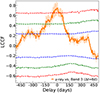 |
Fig. 4. Cross-correlation (LCCF) curve between the band 3 and γ-ray light curves for the whole 8.5 yr period. The dashed blue, green, and red lines are the 68%, 95%, and 99.9% confidence levels, respectively. |
3.3. Evolution of the (sub)mm wave spectral index
Since the band 7 data were quite well sampled (i.e., a median of ∼8 days), we also calculated the spectral index (α) between the bands 3 and 7 flux densities to check the source opacity at (sub)mm wavelengths; in contrast, the sampling of the band 6 data is very poor, which prevented us from using it for a solid analysis. Figure 5 shows the evolution of α between the 95 GHz and 345 GHz emission. The variability timescales of the radio light curves seem to be on month scales overall. To take this into account in the calculations of α, the radio data were binned with multiple bin sizes in the time domain. That is, Bineq ranged from 3 days to 30 days, which corresponds to NBineq sliding from 1038–105. We also tested very small Binseq that varied from from one day to two days. The overall trend was consistent with the result from the larger Bineq range, but with far fewer numbers of the data points. The average of the α values is −0.57 (with 1σ of 0.08), and they range from a minimum of −0.78 to a maximum of −0.19.
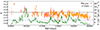 |
Fig. 5. Evolution of the (sub)mm wave radio spectral index (α) between ALMA bands 3 and 7 (i.e., 95 GHz vs. 345 GHz). The horizontal gray line points to α = −0.5. The γ-ray light curve is overlaid in the background for comparison. The horizontal blue line denotes the threshold for the γ-ray flare. |
We considered α ∼ −0.5 as a reference point of the transition between optically thick (flatter; α > −0.5) and thin (steeper; α ≤ −0.5) (Marscher & Gear 1985). Most of the time, the spectral indices are below −0.5 at around −0.6. From visual inspection of Figure 5, however, we found that α becomes flatter (i.e., ≥−0.5) when the γ-rays flare. However, this feature seems to be clearer when the γ-ray flares are stronger and last longer. For the weaker flares, the spectral feature might be less pronounced in the thin regime (i.e., α < −0.5), or they might have a different origin/mechanism without this feature in the (sub)mm wave spectrum. In early 2012 (around MJD 55936), higher γ-rays were observed that perhaps consisted of multiple γ-ray flares. This activity seems marginal or exceeds the flare threshold only slightly. We consider it to be a long-lasting activity (e.g., ≥4 months), but weaker. It is worth noting that there are a few caveats for Figure 5. We note that the sampling of the radio data at both bands 3 and 7 are irregular, and the sampling is quite sparse especially in the early part (i.e., < 2014; MJD 56658). Owing to this, the α values in this early part might be less robust, and care must therefore be taken in this time range. Moreover, there might be hidden fast γ-ray flares (i.e., short-term events on a scale of hours to minutes) that cannot be seen in our γ-ray light curve.
This suggests a connection between the γ-ray flares and the source opacity at (sub)mm wavelengths in the jet (see e.g., Jorstad et al. 2013, for a similar case in the blazar 3C 454.3). Previous studies predicted a rapid decrease in the core shift with increasing radio frequencies (see e.g., Dodson et al. 2017; Lisakov et al. 2017; Okino et al. 2022), for a typical tendency of the core shift profiles). Our finding favors at least a small core shift at above 95 GHz when γ-ray flares occur in the jet of PKS 1424−418.
4. Discussion
4.1. Unusual long-term mm–γ-ray correlation
In general, the detection of a significant mm–γ-ray correlation in blazars has been somewhat intermittent (for light curves spanning about 3–4 yr overall), and only a small number of source samples were reported in previous statistical studies (e.g., Fuhrmann et al. 2014; Max-Moerbeck et al. 2014a; Ramakrishnan et al. 2015, 2016). It is even more difficult to search for these significant correlations in some of the blazars with extreme radio variability (e.g., 0716 + 714, Kim et al. 2022). This is partly because the previous works were done in the low-frequency radio bands (e.g., below 40 GHz) where the radio emission arises from a region that lies farther away from the high-energy region (see Max-Moerbeck et al. 2014a, for their Figure 3). We found a long-term tightly correlated (at > 99.9%) mm–γ-ray variability in PKS 1424−418 that is quite atypical. After the period of our datasets, the source became quiescent at both (sub)mm wavelengths and γ-rays for about one year (e.g., March 2020 to March 2021). Thus, we assume that this unique mm–γ-ray correlation spanned almost ∼10 yr in the source.
Leptonic models (i.e., synchrotron and IC scattering) have been successful in describing most of the blazar SEDs (e.g., Böttcher et al. 2013; Paliya et al. 2018). This tight correlation between γ-ray and lower-energy bands strongly supports the IC processes for the γ-ray emission (e.g., Liodakis et al. 2019) via synchrotron-self Compton (SSC) and/or external Compton (EC) with seed photon fields from either the broad-line region (BLR) or a dusty torus (DT). Previous SED studies indeed favored a combination of the SSC and EC processes for the observed γ-rays from PKS 1424−418 (Tavecchio et al. 2013; Buson et al. 2014; Paliya et al. 2018; Abhir et al. 2021). However, further details about the mechanism are somewhat elusive. Our results refer to a typical diagnostic of the SSC γ-rays (e.g., Agudo et al. 2011b). The strong long-term mm–γ-ray correlation in PKS 1424−418 might be attributed to SSC of low-energy electrons, which leads to longer cooling timescales for the γ-rays (e.g., Böttcher & Baring 2019). However, the significant Compton dominance in this source (e.g., Paliya et al. 2018) indicates that strong external photon fields play an important role via EC (see also Marscher et al. 2010 and MacDonald et al. 2015 for a discussion of a slow jet sheath as a potential source of soft seed photons at ≤ pc scales).
4.2. Location of the γ-ray production site
Based on the stable tight mm–γ-ray correlation over more than 8.5 yr, it is straightforward to consider that the γ-ray origin is cospatial with the (sub)mm wave core region in the jet of PKS 1424−418 (see also van Zyl & Gaylard 2015, for large delays between γ-ray and cm-wavelengths in the source).
The inner jet regions (e.g., < 0.1–1 pc) are thought to be opaque at radio frequencies (Marscher et al. 2008), and radio emission therefore emerges beyond this region where the radio core appears. In blazars, the centimeter-wave core is assumed to be located at 7–12 pc, for instance, from the central engine (Pushkarev et al. 2010; Kramarenko et al. 2022). Thus, the mm wave core is likely to be located at a distance scale smaller than this range, for example, < 7 pc, which is closer to the central engine at higher frequencies. This can be confirmed with mm VLBI observations. For instance, Kim et al. (2023) presented a 3 mm VLBI image of the jet of the blazar BL Lacertae (z = 0.0686) observed by the Global mm VLBI Array (GMVA) on an angular resolution scale of tens of μas (∼70 μas). At this redshift, the image scale of the source is ∼1.3 pc mas−1. Using MBH ∼ 108.2 M⊙ (e.g., Cohen et al. 2014), the angular resolution of 70 μas can be converted into a projected distance of 0.091 pc in the observer frame, which corresponds to ∼6000 Rs, where Rs is the Schwarzschild radius. With the jet viewing angles of 1–10° and assuming a conservative wide range for this blazar (see e.g., Marscher et al. 2008; Weaver et al. 2022), we can obtain a range of the deprojected distance that is ∼0.5–4.9 pc in the source frame. These estimates might be considered as upper limits for the location of the (sub)mm wave core region in BL Lacertae. It is worth noting that Agarwal et al. (2024) recently found an absorption feature in γ-ray spectra of PKS 1424−418 at above 10 GeV (but see also e.g., Costamante et al. 2018, for the absence of such feature in the majority of FSRQs which is a more general case). This might be strong evidence that the γ-rays originated from a region of influence of the BLR photons (e.g., a typical radius of BLR ∼ 0.1 pc). If this is the case, the presence of the γ-ray absorption might either imply the proximity of the (sub)mm wave core to the outer boundary of the BLR or indicated that an extended structure of the BLR lies farther downstream of the jet.
The SSA opacity (τopaq) of a jet region can be enhanced with a higher electron density, which meets the argument of moving shocks in the compact core regions (e.g., Kim et al. 2022). On the other hand, Sharma et al. (2022) presented the effect of the jet viewing angle (θjet) on τopaq in a conical self-absorbed jet. The authors suggested that a spatial displacement between the radio cores with spectral hardening becomes more pronounced at smaller jet viewing angles. This is also consistent with an expression of the SSA opacity (i.e., Finke 2019), that is, τopaq(ϵ)∝δ(p + 2)/2, where ϵ is approximately ∼ ν/(1.23 × 1020) Hz, δ is the Doppler factor, and p is the power-law index of the electrons, α = (p − 1)/2. Thus, there might be a change in θjet near the radio core region and/or a core shift in the (sub)mm waveband during the interaction between the core and the moving shocks (e.g., toward smaller θjet).
4.3. Potential effects of a core shift to the γ-ray origin
The coincidence of the spectral hardening with the γ-ray flares suggests that a gap lies between τγ − B3 and τγ − B7 that was caused by a core shift between 95 GHz and 345 GHz in the jet. To explore this possibility, we examined the LCCF curves of the γ-rays with the bands 3 and 7 datasets (Appendix E). The LCCF curve of the band 7 peaks at two positions: first, at τ = −16 days (LCCF ∼ 0.78 ± 0.15), and then, at τ = 0 (0.77 ± 0.12), where negative τγ − radio means “γ-ray leading”. To better estimate probable locations of the LCCF peaks for both τγ − B3 and τγ − B7, we fit a Gaussian model to the data. The fits estimate τγ − B3 = −2.8 ± 2.0 days and τγ − B7 = −0.8 ± 2.6 days. This result is consistent with the model of the core shift (i.e., the higher the frequencies, the more upstream the regions) and suggests that the γ-rays are almost simultaneous with the band 7 flux densities, but precede the band 3 flux densities by a few days. A cross-correlation analysis is highly dependent on these flux densities in a flaring state (e.g., Kim et al. 2022). As evident from Figure 5, we consider that the source becomes temporarily optically thick at (sub)mm wavelengths during the γ-ray flaring periods. We also note that the photon flux density of blazar γ-ray flares generally tends to be higher with shorter binning intervals. Hence, we cannot rule out the possibility that regions with flatter αradio could cause the weak delay between the band 3 and γ-ray emission. This means that the band 3 emission comes days after the γ-rays and band 7 emission. We also note that the linear relation between the bands 3 and 7 emission shown in Appendix A begins to deviate from an initially tight linear trend at around FB7 ∼ 2.8 Jy. This further supports the above-mentioned interpretation of the variable source opacity at 95–345 GHz. In this regard, we suggest that the γ-ray site and the 95 GHz core position are only slightly displaced when the source is flaring at γ-rays. However, we expect that even this displacement disappears completely at higher radio frequencies (e.g., ≥345 GHz) because the radio core becomes transparent with increasing radio frequency.
The distance (Δdγ − radio) between the mm and γ-ray emitting regions can be estimated by  , where βapp is the apparent jet speed, c is the speed of light, τγ − radio is the delay between radio and γ-ray light curves, θjet is the jet viewing angle, and z is the source redshift. Assuming βapp = 9 (i.e., a median value for FSRQs; Weaver et al. 2022) and θjet = 1–3° (e.g., Paliya et al. 2018; Weaver et al. 2022), we find a deprojected distance of Δdγ − B3 ∼ 0.16 pc with θjet = 3° for τγ − B3 = 2.8 days (Figure 4) and Δdγ − B3 ∼ 0.48 pc with θjet = 1°. This indicates that the γ-ray production site is located in a region upstream of the 95 GHz core by about 0.16–0.48 pc; but if βapp is much higher (e.g., ∼40; Weaver et al. 2022), then the distance range for the same θjet = 1–3° can be Δdγ − B3 ∼ 0.71–2.14 pc. For the τγ − B7 estimate of 0.8 day, it is basically a zero-lag within the uncertainty. If there is at least a small shift in the position of the 345 GHz core and we consider the τγ − B7 of 0.8 day as the corresponding shift, however, the distance between the 345 GHz core and the γ-ray site could be Δdγ − B7 ∼ 0.05–0.14 pc for the same θjet range above at βapp = 9. This distance scale is comparable to the radius of the BLR estimated by Tavecchio et al. (2013).
A simple way to confirm the above predictions is to perform multiband (quasi-)simultaneous VLBI observations of the source at (sub)mm wavelengths to measure the core shift. At z = 1.52, the luminosity distance of PKS 1424−418 is ∼11192 Mpc, and this corresponds to an image scale of 8.54 pc/mas. We find projected distances of ∼0.02 pc or ∼2.5 μas for the Δdγ − B3 values, and if present, ∼0.006 pc or ∼0.7 μas for the Δdγ − B7 values. This suggests that the level of the core shift between the 95 GHz and 345 GHz cores is ∼1.8 μas, which may indeed be present in these high-frequency core regions.
4.4. Physical scenario for the production of the γ-ray flares
From decades of VLBI studies of blazar jets, it is clear that the radio core is a dominant source of the observed radio emission from the jets, especially when a strong disturbance (or a moving shock) passes through the core region (e.g., Marscher et al. 2008). This is particularly true at higher radio frequencies, since there should be no significant contributions from the extended jet regions to the observed radio emission (Marscher & Gear 1985). Higher-energy electrons last much shorter than lower-energy ones regarding their energetic lifetimes. We find remarkable variations in the jet opacity at 95–345 GHz that coincide with the γ-ray flaring periods. Plavin et al. (2019) found a core-shift variability at low frequencies (i.e., 2–8 GHz) with large source samples. This may be related to our findings. As suggested by the authors, the passage of a moving shock through the core region could lead to a displacement in the core position by pushing it downstream. If this holds in our case, the following scenario can be suggested: (1) The radio core was initially optically thin at above 95 GHz (i.e., ≤3.5 mm). (2) A moving shock causes core shifts at (sub)mm wavelengths by temporarily increasing the jet opacity (e.g., Jorstad et al. 2013; Wehrle et al. 2016; Lisakov et al. 2017). (3) As the shock leaves the region, the core restores its initial condition (i.e., opacity and position).
5. Summary
We have studied the time correlation between an mm wave and γ-ray emission in the blazar PKS 1424−418 by using ALMA (sub)mm radio light curves at 90–350 GHz and a LAT γ-ray light curve at 0.1–200 GeV. Because of the cadence of the data sampling, we mainly used ALMA band 3 (∼95 GHz) data with the bands 6 and 7 (235 GHz and 345 GHz, respectively) data as supporting material for the correlation analyses. Interestingly, the band 3 and γ-ray light curves already appear to be very similar to each other visually, and we robustly confirmed this with detailed statistical analyses. We find a highly significant positive mm–γ-ray correlation over the complete time period of 8.5 yr, which means that this blazar is the best case thus far of a long-term close connection between mm wave and γ-ray emission (Marscher, private communication). This long-term strong correlation is typically observed between optical and γ-ray emission in blazars. This suggests that the γ-ray emission almost always originates in the (sub)mm wave radio core region (i.e., > 90 GHz) in this source. If the core shift indeed occurs at the high radio frequencies with strong γ-ray flares, however, an exception can occur when a moving shock passes through the core region. This leads to an increase in the SSA opacity and thus to a displacement between the γ-ray site and the mm wave core. A flare-induced core shift at (sub)mm wavelengths like this could be confirmed by using a multiband VLBI campaign involving extremely high-resolution mm VLBI arrays (see also review by Boccardi et al. 2017) such as GMVA and the Event Horizon Telescope (EHT). It is worthwhile to note that our results are based on a long-term global trend, and there might be other γ-ray events in the source that deviate from our conclusion. A monitoring campaign at shorter mm wavelengths (e.g., < 3.5 mm) with a better sampling cadence (i.e., ≤3 days) would facilitate the investigation of these cases (e.g., orphan γ-ray events).
PSD: A = 0.16 ± 1.20 Hz−1, fbend = 0.004 ± 0.011 Hz, αlow = 0.84 ± 1.04, αhigh = 2.22 ± 0.99, C = 0.10 ± 0.04 Hz−1, and PDF: κ = 17.94 ± 9.42, θ = 0.30 ± 0.15, μ = 1.70 ± 0.03, σ = 0.67 ± 0.04, wΓ = 0.20 ± 0.09. For their mathematical forms, we refer to equations 2 & 3 in Emmanoulopoulos et al. (2013).
Acknowledgments
We thank Alan Marscher & Svetlana Jorstad (Boston University), Yuri Kovalev (MPIfR), and Abhishek Desai & Bindu Rani (GSFC) for useful comments on the manuscript. The Fermi LAT Collaboration acknowledges generous ongoing support from a number of agencies and institutes that have supported both the development and the operation of the LAT as well as scientific data analysis. These include the National Aeronautics and Space Administration and the Department of Energy in the United States, the Commissariat à l’Energie Atomique and the Centre National de la Recherche Scientifique / Institut National de Physique Nucléaire et de Physique des Particules in France, the Agenzia Spaziale Italiana and the Istituto Nazionale di Fisica Nucleare in Italy, the Ministry of Education, Culture, Sports, Science and Technology (MEXT), High Energy Accelerator Research Organization (KEK) and Japan Aerospace Exploration Agency (JAXA) in Japan, and the K. A. Wallenberg Foundation, the Swedish Research Council and the Swedish National Space Board in Sweden. Additional support for science analysis during the operations phase is gratefully acknowledged from the Istituto Nazionale di Astrofisica in Italy and the Centre National d’Études Spatiales in France. This work performed in part under DOE Contract DE-AC02-76SF00515. This paper makes use of the following ALMA data: ADS/JAO.ALMA#2011.0.00001.CAL. ALMA is a partnership of ESO (representing its member states), NSF (USA) and NINS (Japan), together with NRC (Canada), MOST and ASIAA (Taiwan), and KASI (Republic of Korea), in cooperation with the Republic of Chile. The Joint ALMA Observatory is operated by ESO, AUI/NRAO and NAOJ. This research was supported by Basic Science Research Program through the National Research Foundation of Korea (NRF) funded by the Ministry of Education (NRF-2022R1A6A3A03069095). This publication is part of the M2FINDERS project which has received funding from the European Research Council (ERC) under the European Union’s Horizon 2020 Research and Innovation Programme (grant agreement No 101018682). M.K. and F.R. acknowledge funding by the Deutsche Forschungsgemeinschaft (DFG, German Research Foundation) – grant 434448349.
References
- Abdollahi, S., Acero, F., Ackermann, M., et al. 2020, ApJS, 247, 33 [Google Scholar]
- Abdollahi, S., Ajello, M., Baldini, L., et al. 2023, ApJS, 265, 31 [NASA ADS] [CrossRef] [Google Scholar]
- Abhir, J., Joseph, J., Patel, S. R., et al. 2021, MNRAS, 501, 2504 [CrossRef] [Google Scholar]
- Agarwal, S., Shukla, A., Mannheim, K., et al. 2024, ApJ, 968, L1 [NASA ADS] [CrossRef] [Google Scholar]
- Agudo, I., Jorstad, S. G., Marscher, A. P., et al. 2011a, ApJ, 726, L13 [NASA ADS] [CrossRef] [Google Scholar]
- Agudo, I., Marscher, A. P., Jorstad, S. G., et al. 2011b, ApJ, 735, L10 [NASA ADS] [CrossRef] [Google Scholar]
- Ajello, M., Angioni, R., Axelsson, M., et al. 2020, ApJ, 892, 105 [NASA ADS] [CrossRef] [Google Scholar]
- Atwood, W. B., Abdo, A. A., Ackermann, M., et al. 2009, ApJ, 697, 1071 [CrossRef] [Google Scholar]
- Ballet, J., Bruel, P., Burnett, T. H., et al. 2023, ArXiv e-prints [arXiv:2307.12546] [Google Scholar]
- Benke, P., Rösch, F., Ros, E., et al. 2024, A&A, 681, A69 [NASA ADS] [CrossRef] [EDP Sciences] [Google Scholar]
- Blandford, R., Meier, D., & Readhead, A. 2019, ARA&A, 57, 467 [NASA ADS] [CrossRef] [Google Scholar]
- Boccardi, B., Krichbaum, T. P., Ros, E., et al. 2017, A&ARv, 25, 4 [NASA ADS] [CrossRef] [Google Scholar]
- Bonato, M., Liuzzo, E., Giannetti, A., et al. 2018, MNRAS, 478, 1512 [NASA ADS] [CrossRef] [Google Scholar]
- Böttcher, M. 2007, Ap&SS, 309, 95 [CrossRef] [Google Scholar]
- Böttcher, M., & Baring, M. G. 2019, ApJ, 887, 133 [CrossRef] [Google Scholar]
- Böttcher, M., Reimer, A., Sweeney, K., et al. 2013, ApJ, 768, 54 [NASA ADS] [CrossRef] [Google Scholar]
- Buson, S., Longo, F., Larsson, S., et al. 2014, A&A, 569, A40 [NASA ADS] [CrossRef] [EDP Sciences] [Google Scholar]
- Chamani, W., Savolainen, T., Ros, E., et al. 2023, A&A, 672, A130 [NASA ADS] [CrossRef] [EDP Sciences] [Google Scholar]
- Cheung, C. C., Harris, D. E., & Stawarz, Ł. 2007, ApJ, 663, L65 [NASA ADS] [CrossRef] [Google Scholar]
- Cohen, M. H., Meier, D. L., Arshakian, T. G., et al. 2014, ApJ, 787, 151 [Google Scholar]
- Connolly, S. D. 2015, ArXiv e-prints [arXiv:1503.06676] [Google Scholar]
- Costamante, L., Cutini, S., Tosti, G., et al. 2018, MNRAS, 477, 4749 [Google Scholar]
- Dar, A., & Laor, A. 1997, ApJ, 478, L5 [NASA ADS] [CrossRef] [Google Scholar]
- Dodson, R., Rioja, M. J., Molina, S. N., et al. 2017, ApJ, 834, 177 [NASA ADS] [CrossRef] [Google Scholar]
- Edelson, R. A., & Krolik, J. H. 1988, ApJ, 333, 646 [Google Scholar]
- Emmanoulopoulos, D., McHardy, I. M., & Papadakis, I. E. 2013, MNRAS, 433, 907 [NASA ADS] [CrossRef] [Google Scholar]
- Finke, J. D. 2019, ApJ, 870, 28 [NASA ADS] [CrossRef] [Google Scholar]
- Fuhrmann, L., Larsson, S., & Chiang, J. 2014, MNRAS, 441, 1899 [NASA ADS] [CrossRef] [Google Scholar]
- Hodgson, J. A., Rani, B., Lee, S.-S., et al. 2018, MNRAS, 475, 368 [NASA ADS] [CrossRef] [Google Scholar]
- Jorstad, S. G., Marscher, A. P., Mattox, J. R., et al. 2001a, ApJS, 134, 181 [Google Scholar]
- Jorstad, S. G., Marscher, A. P., Mattox, J. R., et al. 2001b, ApJ, 556, 738 [NASA ADS] [CrossRef] [Google Scholar]
- Jorstad, S. G., Marscher, A. P., Smith, P. S., et al. 2013, ApJ, 773, 147 [Google Scholar]
- Kadler, M., Krauß, F., & Mannheim, K. 2016, Nat. Phys., 12, 807 [NASA ADS] [CrossRef] [Google Scholar]
- Keenan, M., Meyer, E. T., Georganopoulos, M., et al. 2021, MNRAS, 505, 4726 [NASA ADS] [CrossRef] [Google Scholar]
- Kim, D.-W., Trippe, S., & Lee, S.-S. 2018, MNRAS, 480, 2324 [NASA ADS] [CrossRef] [Google Scholar]
- Kim, D.-W., Trippe, S., & Kravchenko, E. V. 2020, A&A, 636, A62 [EDP Sciences] [Google Scholar]
- Kim, D.-W., Kravchenko, E. V., Kutkin, A. M., et al. 2022, ApJ, 925, 64 [NASA ADS] [CrossRef] [Google Scholar]
- Kim, D.-W., Janssen, M., Krichbaum, T. P., et al. 2023, A&A, 680, L3 [NASA ADS] [CrossRef] [EDP Sciences] [Google Scholar]
- Kovalev, Y. Y., Aller, H. D., Aller, M. F., et al. 2009, ApJ, 696, L17 [NASA ADS] [CrossRef] [Google Scholar]
- Kramarenko, I. G., Pushkarev, A. B., Kovalev, Y. Y., et al. 2022, MNRAS, 510, 469 [Google Scholar]
- Lee, S.-S., Lobanov, A. P., Krichbaum, T. P., et al. 2008, AJ, 136, 159 [Google Scholar]
- León-Tavares, J., Valtaoja, E., Tornikoski, M., et al. 2011, A&A, 532, A146 [NASA ADS] [CrossRef] [EDP Sciences] [Google Scholar]
- Liodakis, I., Romani, R. W., Filippenko, A. V., et al. 2019, ApJ, 880, 32 [NASA ADS] [CrossRef] [Google Scholar]
- Liodakis, I., Blinov, D., Jorstad, S. G., et al. 2020, ApJ, 902, 61 [NASA ADS] [CrossRef] [Google Scholar]
- Lisakov, M. M., Kovalev, Y. Y., Savolainen, T., et al. 2017, MNRAS, 468, 4478 [NASA ADS] [CrossRef] [Google Scholar]
- Lister, M. L., Aller, H. D., Aller, M. F., et al. 2009, AJ, 137, 3718 [Google Scholar]
- Lobanov, A. P. 1998, A&A, 330, 79 [NASA ADS] [Google Scholar]
- MacDonald, N. R., Marscher, A. P., Jorstad, S. G., et al. 2015, ApJ, 804, 111 [NASA ADS] [CrossRef] [Google Scholar]
- MAGIC Collaboration (Ahnen, M. L., et al.) 2018, A&A, 619, A45 [NASA ADS] [CrossRef] [EDP Sciences] [Google Scholar]
- Marscher, A. P. 2016, Galaxies, 4, 37 [NASA ADS] [CrossRef] [Google Scholar]
- Marscher, A. P., & Gear, W. K. 1985, ApJ, 298, 114 [Google Scholar]
- Marscher, A. P., Jorstad, S. G., D’Arcangelo, F. D., et al. 2008, Nature, 452, 966 [Google Scholar]
- Marscher, A. P., Jorstad, S. G., Larionov, V. M., et al. 2010, ApJ, 710, L126 [Google Scholar]
- Max-Moerbeck, W., Hovatta, T., Richards, J. L., et al. 2014a, MNRAS, 445, 428 [Google Scholar]
- Max-Moerbeck, W., Richards, J. L., Hovatta, T., et al. 2014b, MNRAS, 445, 437 [NASA ADS] [CrossRef] [Google Scholar]
- Nair, D. G., Lobanov, A. P., Krichbaum, T. P., et al. 2019, A&A, 622, A92 [NASA ADS] [CrossRef] [EDP Sciences] [Google Scholar]
- Okino, H., Akiyama, K., Asada, K., et al. 2022, ApJ, 940, 65 [NASA ADS] [CrossRef] [Google Scholar]
- Paliya, V. S., Zhang, H., Böttcher, M., et al. 2018, ApJ, 863, 98 [Google Scholar]
- Plavin, A. V., Kovalev, Y. Y., Pushkarev, A. B., et al. 2019, MNRAS, 485, 1822 [NASA ADS] [CrossRef] [Google Scholar]
- Pushkarev, A. B., Kovalev, Y. Y., & Lister, M. L. 2010, ApJ, 722, L7 [NASA ADS] [CrossRef] [Google Scholar]
- Ramakrishnan, V., Hovatta, T., & Nieppola, E. 2015, MNRAS, 452, 1280 [CrossRef] [Google Scholar]
- Ramakrishnan, V., Hovatta, T., & Tornikoski, M. 2016, MNRAS, 456, 171 [NASA ADS] [CrossRef] [Google Scholar]
- Rani, B., Jorstad, S. G., Marscher, A. P., et al. 2018, ApJ, 858, 80 [Google Scholar]
- Röder, J., Ros, E., Schinzel, F. K., et al. 2024, A&A, 684, A211 [NASA ADS] [CrossRef] [EDP Sciences] [Google Scholar]
- Sharma, R., Massi, M., & Torricelli-Ciamponi, G. 2022, A&A, 660, A58 [NASA ADS] [CrossRef] [EDP Sciences] [Google Scholar]
- Tavecchio, F., Pacciani, L., Donnarumma, I., et al. 2013, MNRAS, 435, L24 [CrossRef] [Google Scholar]
- van Zyl, P. V., & Gaylard, M. J. 2015, Mem. Soc. Astron. It., 86, 36 [NASA ADS] [Google Scholar]
- Weaver, Z. R., Jorstad, S. G., Marscher, A. P., et al. 2022, ApJS, 260, 12 [NASA ADS] [CrossRef] [Google Scholar]
- Wehrle, A. E., Marscher, A. P., Jorstad, S. G., et al. 2012, ApJ, 758, 72 [Google Scholar]
- Wehrle, A. E., Grupe, D., Jorstad, S. G., et al. 2016, ApJ, 816, 53 [Google Scholar]
- Welsh, W. F. 1999, PASP, 111, 1347 [Google Scholar]
- White, G. L., Jauncey, D. L., Savage, A., et al. 1988, ApJ, 327, 561 [NASA ADS] [CrossRef] [Google Scholar]
Appendix A: The ALMA band 3, 6, and 7 data
Although the data sampling is best in the band 3 (B3), we were able to obtain useful radio light curves of the source at other ALMA bands: band 6 (B6; ∼235 GHz) and band 7 (B7; ∼345 GHz). Their sampling intervals are, on average, ∼66 days with a median value of ∼25 days at band 6 and ∼14 days with a median value of ∼8 days at band 7. Figure A.1 shows all the ALMA light curves of the source. For every pair of the two time series (i.e., B3–B6, B6–B7, and B7–B3), we calculated the Pearson correlation coefficients following the manner described in Appendix B. The Bineq ranges were set to be 3–30 days for the B7–B3 pair (i.e., ∼930 flux–flux sets) and 3–15 days for the other two pairs with band 6 (i.e., ∼830 flux–flux sets). This is due to the poor sampling of the band 6 data which is significantly worse (e.g., 4–5 times) than the other two bands. The Bineq ranges correspond to NBineq of ∼1040 to ∼110 for B7–B3 and ∼1040 to ∼210 for the others. The results on the three pairs are shown in Figure A.1. We find the averages of rP as follow: 0.967±0.004 (with 1 σ uncertainty) for B3–B7, 0.987±0.002 for B3–B6, and 0.988±0.005 for B7–B6.
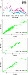 |
Fig. A.1. From top to bottom: ALMA light curves of PKS 1424−418 at band 3 (95 GHz), band 6 (235 GHz), and band 7 (345 GHz) and plots of the flux–flux scatter (∼930 samples for B7–B3 & ∼830 samples for the others) for each pair of the ALMA bands. |
Appendix B: Testing Pearson correlation
We investigated linear relationships between the light curves by using the Pearson correlation. For each pair of two time series (e.g., mm & γ-ray), we determined a time range of the data where it begins at the minimum of the two time series and ends at the maximum of the two time series. The full time range was divided into equal-sized bins (Bineq) to account for the uneven and random distribution of the data. To ensure accuracy, this test was repeated in a range of different sizes of Bineq, taking into account the data sampling and source variability; NBineq is the total number of Bineq in a single test run. We calculated an average of all the flux densities belonging to each of the Bineq and used it as a typical flux density for each of them. Once this process is done throughout all NBineq on the two light curves separately, we only selected Bineq overlapping with each other and calculated a Pearson correlation coefficient (rP) by using these selected local-mean flux densities.
Appendix C: Cross-correlation analysis
The Discrete Correlation Function (DCF; Edelson & Krolik 1988) has been widely employed in the analysis of time-correlation between two light curves. To avoid the normalization issues of DCF (i.e., Max-Moerbeck et al. 2014b), however, we employed the Local Cross-Correlation Function (LCCF; e.g., Welsh 1999) in this work. We compute the cross-correlation coefficients with the following DCF and LCCF functions:
![Mathematical equation: $$ \begin{aligned}&DCF (\tau ) = M^{-1}\,\left[\frac{\sum (a_{i} - \bar{a}_{0})(b_{j} - \bar{b}_{0})}{\sigma _{a\,0}\,\sigma _{b\,0}}\right], \\&LCCF (\tau ) = M^{-1}\,\left[\frac{\sum (a_{i} - \bar{a}_{\tau })(b_{j} - \bar{b}_{\tau })}{\sigma _{a\,\tau }\,\sigma _{b\,\tau }}\right], \end{aligned} $$](/articles/aa/full_html/2024/12/aa51773-24/aa51773-24-eq2.gif) (C.1)
(C.1)
where ai & bj being two time series,  &
&  the mean values for the time series, σa 0 & σb 0 the standard deviation values for the time series, and M the number of (i, j) pairs that fall within the delay bin defined as τ − Δt/2 ≤ Δtij < τ + Δt/2; here τ and Δt refer to time delay and a size of the delay bin, respectively.
  ,
,  , σa τ, and σb τ are the same as above, but only for those M overlapping samples. We determine the uncertainties i.e., σDCF(τ) and σLCCF(τ) by measuring a statistical dispersion for each DCF(τ) and LCCF(τ), respectively (see e.g., Max-Moerbeck et al. 2014b). The main difference between the two approaches is that LCCF only considers data points overlapping within the delay bin between two time series.
Max-Moerbeck et al. (2014b) made a comparison between DCF and LCCF, and concluded that LCCF is better than DCF in terms of e.g., detection efficiency. For more details of the comparison, we refer to Max-Moerbeck et al. (2014b). We also tested these two functions with our datasets. Figure C.1 shows the result. As evident from it, the LCCF curve returns higher coefficient values. Both the LCCF and DCF curves peaked at τ = 0. However, we find that the peak of the LCCF curve is much closer to the mean of the Pearson coefficients presented in Figure 3. Thus, we consider that LCCF is a more accurate way to search for time-correlation in this study.
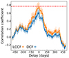 |
Fig. C.1. Comparison between LCCF and DCF. The γ-ray and ALMA band 3 light curves shown in Figure 2 were used in this test (Δt = 6 days for both the correlation curves). The red dashed line indicates the average rP value of Figure 3. |
We evaluated the resultant LCCF curves by using their confidence levels. The overall procedure is similar to the manner of Kim et al. (2022). We simulated 100,000 artificial γ-ray light curves and computed LCCF curves between those simulated γ-rays and the observed ALMA band 3 light curve. For every τ, we draw a cumulative distribution function (CDF) of the correlation coefficients and find the 68%, 95%, and 99.9% confidence levels. Based on these confidence levels, we determine the significance of the LCCF peaks.
The artificial γ-ray light curves were generated in the manner of Emmanoulopoulos et al. (2013). Most of the time, PKS 1424−418 was bright at γ-rays and there are a small number of bad/empty bins. Using linear interpolation, we complemented these bins and thus made the light curve evenly distributed. Then, we find a power spectral density (PSD) and a probability density function (PDF) of the γ-rays with this interpolated light curve. A bending power-law model and the mixture model (i.e., a combination of the gamma and log-normal distributions) introduced by Emmanoulopoulos et al. (2013), were applied to a periodogram and histogram of the data, respectively. Figure C.2 shows the best-fit PSD and PDF models. Then, the artificial γ-ray light curves were generated with a Python implementation DELCgen (Connolly 2015) that follows the algorithm of Emmanoulopoulos et al. (2013), by using the estimated PSD & PDF parameters 5. Finally, we modified the sampling of all the artificial γ-ray light curves to make them the same as the observed γ-ray light curve in the time domain.
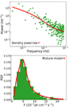 |
Fig. C.2. Best-fit PSD (upper) and PDF (lower) models (in red color) of the γ-rays. |
Appendix D: Tests on the LCCF curves
Figure D.1 shows the LCCF curves between the γ-ray and ALMA band 3 light curves with larger Δt values (i.e., 12, 30, and 60 days). We find again a significant (i.e., > 99.9%), strong mm–γ-ray correlation at around τ = 0 (zero-lag). The overall shape of the LCCF curves are consistent with each other. However, those statistical fluctuations along the curves become smoother and weaker with increasing Δt. Some of the small humps (e.g., the one at around τ ∼ −120 days) completely disappear with Δt = 60 days. They could be artifacts or short-term, local correlations. Thus, higher Δt values could be helpful to identify a long-term correlation that remains throughout the whole period of the data.
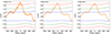 |
Fig. D.1. LCCF curves (in orange color) between the ALMA band 3 and γ-ray light curves of PKS 1424−418 over the whole 8.5 yr. From left to right: Δt = 12, 30, and 60 days. The blue, green, and red dashed lines are the 68%, 95%, and 99.9% confidence levels. |
Appendix E: Gaussian fit to the LCCF curves
In Figure E.1, we fit a single Gaussian to the LCCF curve between the LAT and ALMA band 7 light curves; we omitted the confidence levels for clarity, but the central hump is also above the 99.9% level. Δt was set to be 8 days that is the median sampling of the band 7 light curve. To better fit the model to the data and focus on the significant central LCCF hump, we only used the LCCF points higher than the peak of a first strong, distinct side-lobe (i.e., LCCF = ∼0.48). The result can be found in the upper panel of Figure E.2. We also estimate a peak position of the LCCF hump between the LAT and band 3 light curves (i.e., Figure 4), by using the same manner as Figure E.1. We show the result in the lower panel of Figure E.2. Owing to the poor sampling of the band 6, we skip the band 6 data in the LCCF analysis; the statistical fluctuations and huge side-lobes occupy the LCCF curve between the LAT and band 6 data throughout the whole τ values. We note that the Gaussian model well describes both the LCCF curves shown above, and the results are irrelevant to the bin size (Δt).
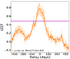 |
Fig. E.1. LCCF curve (Δt = 8 days) between the γ-ray and ALMA band 7 light curves, over the whole 8.5 yr. The data points above LCCF ∼ 0.48 (i.e., the purple horizontal solid line) were used in the fit. |
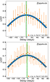 |
Fig. E.2. Top: Zoom-in-view of Figure E.1 shows the details of the fit results. The blue curve indicates the best-fit Gaussian model with a peak location of −0.8±2.6 days (marked by the green dashed line with gray shaded area). Bottom: Same as the above, but between the γ-ray and ALMA band 3 light curves. In Figure 4, the values above LCCF ∼ 0.52 were used in the fit. The estimated Gaussian peak is at −2.8±2.0 days. |
All Figures
|
Fig. 1. Power-law index vs. time (upper) and flux density (lower) of the γ-ray emission of PKS 1424−418. The black lines in each panel indicate the median values on each axis: Γmedian = −2.17 and Fmedian = 5.39 × 10⁻⁷ ph cm−2 s−1. |
| In the text | |
|
Fig. 2. ALMA band 3 (95 GHz) light curve (upper) and 6-day-binned LAT γ-ray light curve (lower) of PKS 1424−418 in 2011–2020 (∼8.5 yr). The red arrows indicate the 2σ upper limits of the γ-rays. The detection of γ-ray photons in terms of TS is shown as the light orange line. The horizontal blue line denotes the threshold for the γ-ray flare. |
| In the text | |
|
Fig. 3. Pearson correlation tests between the ALMA band 3 and LAT light curves for the whole 8.5 yr period. We estimated 488 different Pearson coefficients (rP) using different time-grids (see Appendix B). Upper panel: rP distribution on different scales of the time bin. The dashed red lines refer to the highest rP value (i.e., ∼0.86) at Bineq = 69.1 days (NBineq = 46). Lower panel: Flux–flux scatters corresponding to the rP estimates shown in the upper panel. The scatter for the highest rP is shown in red. The transparency of the data points is set to be very high (thus faint) to highlight the points that appear more frequently. |
| In the text | |
|
Fig. 4. Cross-correlation (LCCF) curve between the band 3 and γ-ray light curves for the whole 8.5 yr period. The dashed blue, green, and red lines are the 68%, 95%, and 99.9% confidence levels, respectively. |
| In the text | |
|
Fig. 5. Evolution of the (sub)mm wave radio spectral index (α) between ALMA bands 3 and 7 (i.e., 95 GHz vs. 345 GHz). The horizontal gray line points to α = −0.5. The γ-ray light curve is overlaid in the background for comparison. The horizontal blue line denotes the threshold for the γ-ray flare. |
| In the text | |
|
Fig. A.1. From top to bottom: ALMA light curves of PKS 1424−418 at band 3 (95 GHz), band 6 (235 GHz), and band 7 (345 GHz) and plots of the flux–flux scatter (∼930 samples for B7–B3 & ∼830 samples for the others) for each pair of the ALMA bands. |
| In the text | |
|
Fig. C.1. Comparison between LCCF and DCF. The γ-ray and ALMA band 3 light curves shown in Figure 2 were used in this test (Δt = 6 days for both the correlation curves). The red dashed line indicates the average rP value of Figure 3. |
| In the text | |
|
Fig. C.2. Best-fit PSD (upper) and PDF (lower) models (in red color) of the γ-rays. |
| In the text | |
|
Fig. D.1. LCCF curves (in orange color) between the ALMA band 3 and γ-ray light curves of PKS 1424−418 over the whole 8.5 yr. From left to right: Δt = 12, 30, and 60 days. The blue, green, and red dashed lines are the 68%, 95%, and 99.9% confidence levels. |
| In the text | |
|
Fig. E.1. LCCF curve (Δt = 8 days) between the γ-ray and ALMA band 7 light curves, over the whole 8.5 yr. The data points above LCCF ∼ 0.48 (i.e., the purple horizontal solid line) were used in the fit. |
| In the text | |
|
Fig. E.2. Top: Zoom-in-view of Figure E.1 shows the details of the fit results. The blue curve indicates the best-fit Gaussian model with a peak location of −0.8±2.6 days (marked by the green dashed line with gray shaded area). Bottom: Same as the above, but between the γ-ray and ALMA band 3 light curves. In Figure 4, the values above LCCF ∼ 0.52 were used in the fit. The estimated Gaussian peak is at −2.8±2.0 days. |
| In the text | |
Current usage metrics show cumulative count of Article Views (full-text article views including HTML views, PDF and ePub downloads, according to the available data) and Abstracts Views on Vision4Press platform.
Data correspond to usage on the plateform after 2015. The current usage metrics is available 48-96 hours after online publication and is updated daily on week days.
Initial download of the metrics may take a while.