| Issue |
A&A
Volume 692, December 2024
|
|
|---|---|---|
| Article Number | A108 | |
| Number of page(s) | 10 | |
| Section | Cosmology (including clusters of galaxies) | |
| DOI | https://doi.org/10.1051/0004-6361/202451640 | |
| Published online | 03 December 2024 | |
Measuring the intracluster medium velocity structure within the A3266 galaxy cluster
1
Max-Planck-Institut für Extraterrestrische Physik, Gießenbachstraße 1, 85748 Garching, Germany
2
Institute of Astronomy, Madingley Road, Cambridge, CB3 0HA, UK
3
INAF – IASF Palermo, Via U. La Malfa 153, I-90146 Palermo, Italy
4
School of Physics & Astronomy, University of Nottingham, University Park, Nottingham, NG7 2RD, UK
5
Department of Astronomy, University of Geneva, Ch. d’Ecogia 16, CH-1290 Versoix, Switzerland
6
Department of Physics and Astronomy, University of Alabama in Huntsville, Huntsville, AL 35899, USA
7
Harvard-Smithsonian Center for Astrophysics, 60 Garden Street, Cambridge, MA 02138, USA
8
Department of Astrophysical Sciences, Princeton University, NJ, 08544, USA
⋆ Corresponding author; This email address is being protected from spambots. You need JavaScript enabled to view it.
Received:
24
July
2024
Accepted:
6
November
2024
Abstract
We present a detailed analysis of the velocity structure of the hot intracluster medium (ICM) within the A3266 galaxy cluster, including new observations taken between June and November 2023. Firstly, morphological structures within the galaxy cluster were examined using a Gaussian gradient magnitude (GGM) and an adaptively smoothed GGM filter applied to the EPIC-pn X-ray image. Then, we applied a novel XMM-Newton EPIC-pn energy scale calibration, which uses instrumental Cu Kα as a reference for the line emission, to measure the line-of-sight velocities of hot gas within the system. This approach enabled us to create two-dimensional projected maps for velocity, temperature, and metallicity, showing that the hot gas displays a redshifted systemic velocity relative to the cluster redshift across all fields of view. Further analysis of the velocity distribution through non-overlapping circular regions demonstrates consistent redshifted velocities extending up to 1125 kpc from the cluster core. Additionally, the velocity distribution was assessed along regions following surface brightness discontinuities, where we observed redshifted velocities in all regions, with the largest velocities reaching 768 ± 284 km/s. Moreover, we computed the velocity probability density function (PDF) from the velocity map. We applied a normality test, finding that the PDF adheres to an unimodal normal distribution consistent with theoretical predictions. Lastly, we computed a velocity structure function for this system using the measured line-of-sight velocities. These insights advance our understanding of the dynamic processes within the A3266 galaxy cluster and contribute to our broader knowledge of ICM behavior in merging galaxy clusters.
Key words: galaxies: clusters: intracluster medium / galaxies: clusters: individual: A3266 / X-rays: galaxies: clusters
© The Authors 2024
 Open Access article, published by EDP Sciences, under the terms of the Creative Commons Attribution License (https://creativecommons.org/licenses/by/4.0), which permits unrestricted use, distribution, and reproduction in any medium, provided the original work is properly cited.
This article is published in open access under the Subscribe to Open model.
Open Access funding provided by Max Planck Society.
1. Introduction
The intracluster medium (ICM) is a hot, ionized gas that fills the space between galaxies in a cluster, emitting X-rays due to its high temperature of several million kelvins. Measuring the velocities of the ICM is crucial for several reasons. Turbulent motions provide additional pressure support, particularly at large radii, affecting cluster mass estimates and calculations of hydrostatic equilibrium (Lau et al. 2009). Simulations predict a close connection between entropy, temperature, density, and velocity power spectra, which should be tested (Gaspari et al. 2014). Velocity measurements can help to constrain active galactic nucleus (AGN) feedback models, as the distribution of energy from AGN feedback within the cluster depends on the balance between turbulence, sound waves, shocks, gravity waves, supernova explosions, and cosmic rays (McNamara & Nulsen 2012). Additionally, these motions contribute to the transport of metals within the ICM through processes such as the uplift caused by AGN (e.g., Simionescu et al. 2008) and gas sloshing (Ascasibar & Markevitch 2006). The microphysics of the ICM, including viscosity, can also be probed by measuring velocities (ZuHone et al. 2016, 2018). Furthermore, velocity measurements can directly detect the transition of the gas within cold fronts, which can persist for several gigayears (Ascasibar & Markevitch 2006).
The Hitomi observatory directly measured random and bulk motions in the ICM using the Fe-K emission lines, thanks to its high-spectral-resolution microcalorimeter Soft X-ray Spectrometer (SXS) X-ray detector. In the core of the Perseus cluster, it measured a bulk flow gradient of 150 km/s across 60 kpc of the cluster core and a line-of-sight velocity dispersion of 164 ± 10 km/s between radii of 30 − 60 kpc (Hitomi Collaboration 2016). These results, obtained for a very limited spatial region, show that the Perseus core is not strongly turbulent, despite the apparent impact of the AGN and its jets on the surrounding ICM and the merger-driven sloshing motions. Such a low level of turbulence suggests that it does not provide distributed heating, although sound waves or shocks could plausibly do this as well as heating from merging activity (Fabian et al. 2017). Unfortunately, no further measurements were made in other clusters or different regions of Perseus due to the loss of Hitomi. However, the new XRISM mission is expected to extend the Fe K velocity measurements in more clusters.
Suzaku also obtained velocity measurements in several systems using the Fe-K line, thanks to its accurate calibration. Tamura et al. (2014) placed upper limits on relative velocities of 300 km/s over scales of 400 kpc in Perseus. Ota & Yoshida (2016) examined several clusters with Suzaku, though systematic errors from the calibration were likely around 300 km/s, and its point spread function was large. Other methods of measuring velocities include using XMM-Newton RGS spectra to measure line widths (e.g., Pinto et al. 2015) and examining resonant scattering (e.g., Ahoranta et al. 2016), both of which are limited to the cluster core. Indirect measurements of velocity structure in clusters include analyzing the power spectrum of density fluctuations and linking this via simulations to the velocity spectrum (e.g., Zhuravleva et al. 2014), or examining the magnitude of thermodynamic perturbations (Hofmann et al. 2016). However, these methods are model-dependent.
Sanders et al. (2020, hereafter SAN+20) present a novel technique using background X-ray lines observed in the spectra of the XMM-Newton EPIC-pn detector to calibrate the absolute energy scale of the detector to better than 150 km/s at Fe-K. Using this technique, SAN+20 mapped the bulk velocity distribution of the ICM over a large fraction of the Perseus and Coma clusters. For the Perseus cluster, they detected evidence of sloshing associated with a cold front. In the Coma cluster, SAN+20 found that the gas velocity closely matches the optical velocities of the two central galaxies, NGC 4874 and NGC 4889. However, the velocity structure near the cluster center was not studied for either source due to the lack of offset observations covering the central region.
In recent years, four large XMM-Newton observation programs were approved to observe the Virgo, Centaurus, and Ophiuchus clusters and apply this method. Using this technique, we have obtained accurate velocity measurements with uncertainties down to Δv ∼ 100 km/s. The analysis of the Virgo cluster shows signatures of both AGN outflows and gas sloshing in the velocity field of the cluster (Gatuzz et al. 2022a). For the Centaurus cluster, we have found (a) an overall gradient in velocities at large radii, (b) a complex velocity profile near the cluster center, and (c) changes in velocities along the cold fronts (Gatuzz et al. 2022b). In the Ophiuchus cluster, we have identified a large redshifted-blueshifted interface located approximately 150 kpc east of the cluster core (Gatuzz et al. 2023a). This interface, which shows signs of a lack of metal mixing, is traced by discontinuities in the X-ray surface brightness. These large observational campaigns also allow us to measure the velocity structure function (VSF) within the systems (Gatuzz et al. 2023b). The VSFs constitute a useful diagnostic tool for studying the turbulence in a medium since they represent the velocity variation with scale (Federrath et al. 2010, 2021; Seta et al. 2023). Furthermore, a detailed analysis of the metallicity distribution in the context of the velocity structure has been carried out for these sources (Gatuzz et al. 2023c, 2023d, 2023e).
The A3266 galaxy cluster is an excellent candidate for studying the ICM velocity distribution. It is one of the most brilliant clusters in the sky (Edge et al. 1990) and one of the brightest merging clusters with temperatures exceeding 7 keV. ASCA observations of the cluster provide evidence of a merger, detecting a temperature variation along the merger axis (Henriksen et al. 2000). Chandra observations identified a cooler filamentary region centered on the central cD galaxy and aligned along the merger axis (Henriksen & Tittley 2002). Finoguenov et al. (2006) estimated the mass of this cooler, denser material to be 1.3 × 10¹³ M⊙ with high metallicity using XMM-Newton observations, suggesting that it results from a merger with a mass ratio of 1:10. Sauvageot et al. (2005) proposed a similar scenario, attributing the low-entropy material to a merger in a direction close to the plane of the sky.
Numerical simulations computed by Sauvageot et al. (2005) present two possible scenarios for the merger: the subcluster may have entered from the southwest, passing the core 0.8 Gyr ago and now nearing turnaround, or it could have merged from the northeast and is now exiting to the southwest after passing the core 0.15–0.20 Gyr ago. Ettori et al. (2019) analyzed XMM-Newton data out to the cluster’s virial radius, finding masses of M500 = 8.8 × 10¹⁴ M⊙ and M200 = 15 × 1014 M⊙, with radii of R500 = 1.43 Mpc and R200 = 2.33 Mpc, assuming a Navarro–Frenk–White (NFW) mass model (Navarro et al. 1996). Dehghan et al. (2017) measured spectroscopic redshifts of 1300 sources within the cluster, identifying that the cluster core, which can be split into two components, decomposes into six groups and filaments to the north. They conclude that a range of continuous dynamical interactions occur, rather than a simple northeast-southwest merger.
A3266 was the target of a calibration observation for the new eROSITA X-ray telescope (Predehl et al. 2021) during its calibration and performance verification phase (Dennerl et al. 2020). In their data analysis, Sanders et al. (2022) confirmed that the source is not a simple merging cluster. Instead, it involves three different systems merging with the main body: the northeastern structure, the northwestern structure, and the western structure. These systems are seen as low-entropy material associated with higher-metallicity gas. However, the data did not conclusively reveal whether there is a merger shock on the west side of the central core. Pressure jumps in the southeast and west directions were identified toward the outskirts of the cluster. The presence of several subclusters that are merging or will soon merge makes A3266 an ideal laboratory for a detailed study of the ICM velocity structure within such a system.
We present an analysis of the ICM velocity structure within the A3266 galaxy cluster using XMM–Newton observations. The outline of this paper is as follows. We describe the data reduction process in Sect. 2 and analyze the X-ray images in Sect. 3. The fitting procedure and the results are shown in Sect. 4, while a discussion of the results is included in Sect. 5. Finally, Sect. 6 presents the conclusions and summary. Throughout this paper, we assume the distance of A3266 to be z = 0.0594 (Dehghan et al. 2017) and a concordance ΛCDM cosmology with Ωm = 0.3, ΩΛ = 0.7, and  .
.
2. A3266 XMM-Newton observations
We analyzed eight A3266 observations taken between June and November 2023 (PI: E. Gatuzz, ID:092188). Additionally, we included ten observations that are available in the archive. Table 1 lists information on the observations, including IDs, coordinates, dates, and clean exposure times. All XMM-Newton European Photon Imaging Camera (EPIC-pn, Strüder et al. 2001) spectra were reduced with the Science Analysis System (SAS1, version 19.1.0). We processed the observations with the epchain SAS tool, including only single-pixel events (PATTERN==0) and filtering the data with FLAG==0 to avoid bad pixels and regions close to CCD edges. A 1.0 cts/s rate threshold was applied to filter out bad time intervals from flares.
XMM-Newton observations of the A3266 cluster.
To measure the velocity structure within the A3266 cluster, we applied the technique described in Sanders et al. (2020) and Gatuzz et al. (2022a) to calibrate the absolute energy scale of the EPIC-pn detector using the instrumental background X-ray lines identified in the detector spectra. This calibration method includes corrections for (1) the average gain of the detector during the observation, (2) the spatial gain variation across the detector over time, and (3) the energy scale as a function of the detector position and time. We created X-ray images and identified point sources using the SAS task edetect_chain, with a likelihood parameter det_ml > 10. In the following analysis, we have excluded the point sources.
3. X-ray images
The top panel of Fig. 1 shows an RGB image of the cluster, with energy bands corresponding to 0.2–0.5 keV (R), 0.5–1.0 keV (G), and 1.0–2.0 keV (B). The exposure-corrected images were smoothed with a Gaussian of σ = 1. The bottom panel of Fig. 1 displays the X-ray exposure-corrected image in the 0.5–9.25 keV energy band. A Gaussian smoothing of σ = 4 pixels was applied, and the 10-level contour of the X-ray image is shown in white.
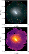 |
Fig. 1. RGB and X-ray images of the A3266 cluster. Top panel: RGB image of A3266. The bands used are 0.2–0.5 keV (R), 0.5–1.0 keV (G), and 1.0–2.0 keV (B). We applied a σ = 1 Gaussian smoothing to the exposure-corrected and background-subtracted image. Bottom panel: Exposure-corrected and background-subtracted X-ray surface brightness of the A3266 cluster in the 0.5–9.25 keV energy range. The point-like sources were excluded in the analysis. The 10-level contours of the X-ray image are shown in white. |
The top panel of Fig. 2 shows the total exposure time in the 4.0–9.25 keV energy range. The middle panel displays the normalized number of counts in each 1.59 arcsec pixel within the Fe-K complex (6.50–6.90 keV) after subtracting the neighboring continuum images (6.06–6.43 keV and 6.94–7.16 keV, the rest frame). The instrumental Cu ring is included to indicate regions in which the redshift can be measured. This image demonstrates a good distribution of counts in the cluster center region, allowing for detailed analysis of the Fe-K complex. The bottom panel shows the normalized number of counts in each 1.59 arcsec pixel around the Cu background line. The plot reveals the Cu hole described in Sanders et al. (2020) for each exposure. Since velocity measurements can only be obtained using the Cu background line, it is crucial to have many counts in regions where the Fe-K complex redshift will be measured.
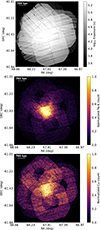 |
Fig. 2. Exposure maps and Fe, Cu counts map for the A3266 cluster. Top panel: Total exposure time (s) in the 0.5–9.25 keV energy range. Middle panel: Normalized Fe-K count map, showing the number of counts in each 1.59 arcsec pixel in the Fe-K complex with the instrumental Cu ring included to indicate the regions in which the redshift can be measured. Bottom panel: Normalized background Cu count map, showing the number of counts in each 1.59 arcsec pixel in the Cu Kα line energy range. |
To study the structures within the galaxy cluster in detail, we filtered the data using a GGM filter (GGM, Sanders et al. 2016a, 2016b). Figure 3 shows the gradient magnitude of the X-ray image convolved with Gaussians of scales of 4 pixels (8 arcsec, top panel) and 8 pixels (16 arcsec, bottom panel). Point sources were cosmetically filled using the values of neighboring pixels before filtering. A 700-800 kpc elliptical surface brightness edge surrounding the core is clearly shown. The image does not accurately depict the relative magnitudes of features but highlights these structures.
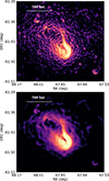 |
Fig. 3. Edge-filtered X-ray images using a Gaussian gradient magnitude (GGM) filter on scales of 4 pixels (top panel) and 8 pixels (bottom panel). |
We also applied the adaptively smoothed GGM filter developed in Sanders et al. (2022). The image and exposure map were convolved to apply this filter by a Gaussian with a σ corresponding to a radius containing 1024 counts. The log10 value of this map was then taken, and the gradient was calculated by taking the difference between neighboring pixels along the two axes and adding them in quadrature. Figure 4 shows the resulting image, clearly revealing the sharp edge near the cluster core.
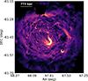 |
Fig. 4. Edge-filtered X-ray images using an adaptive Gaussian gradient magnitude (GGM) filter from Sanders et al. (2022) using a signal-to-noise ratio of 32, where the scale shows the gradient as the log(10) change per 4 arcsec pixel. |
Figure 5 shows the fractional difference in the 0.5–2 keV surface brightness from the average at each radius. The black regions correspond to point-like sources whose sizes have increased artificially due to image smoothing. The X-ray image was smoothed by a 2σ Gaussian. Multiple clear, sharp discontinuities are visible, which have also been identified by Sanders et al. (2022). We analyze these structures in detail in Sect. 4.3.
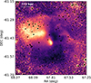 |
Fig. 5. Subtracted fractional difference from the average at each radius for the 0.5–2 keV X-ray surface brightness. The point-like sources were excluded in the analysis. The X-ray image was smoothed by a 2σ Gaussian. |
4. Spectral fitting procedure
The spectra were fit in the 4.0–9.25 keV energy band. We combined the spectra from different observations for each spatial region analyzed, using the number of counts in the fitting spectral region as the weighting factor. We modeled the ICM X-ray emission with version 3.0.9 of the apec thermal emission model (Foster et al. 2019), which includes corrections derived from the Hitomi observations (Hitomi Collaboration 2018). A tbabs component (Wilms et al. 2000) was also included to account for the Galactic X-ray absorption, corresponding to 2.26 × 1020 cm−2 (Kalberla et al. 2005). However, we note that for the energy range analyzed, the absorbing component does not affect the modeling (Gatuzz et al. 2022a, 2022b, 2023a). The free parameters in the model are the temperature, metallicity (i.e., metal abundances with He fixed at cosmic levels), redshift, and normalization.
For the X-ray spectral fits, we used the XSPEC data fitting package (version 12.14.02). We assumed cash statistics (Cash 1979). Errors are quoted at a 1-σ confidence level unless otherwise stated. Abundances are given relative to Lodders et al. (2009). As background components, we included Cu-Kα, Ni-Kα, Zn-Kα, and Cu-Kβ instrumental emission lines, as well as a power-law component with its photon index fixed at 0.136 (the average value obtained from the archival observations analyzed in Sanders et al. 2020).
4.1. Spectral maps
We created maps of the cluster spectral properties using a method developed in Sanders et al. (2020), based on fitting spectra from dynamically sized ellipses. To create these maps, we rotated elliptical regions with a 2:1 axis ratio so that the longest axis lies tangentially to the vector pointing to the central core. The radii of the ellipses adaptively change in a grid with a spacing of 0.25 arcmin to achieve approximately 1000 counts in the Fe-K complex after continuum subtraction, thereby reducing the velocity uncertainties. The semi-major axis ranges from 6.1 arcmin to 2.0 arcmin. We combined the spectra obtained per region for all observations and created weighted-average ancillary response files, while using the same response matrix for all the pixels. The spectra were then fit as is described in Sect. 4.
Figure 6 shows the velocity map (top panel), the velocity uncertainties (middle panel), and the significance of the velocity measurements (bottom panel) obtained. We use a blue-red color scale for the velocity map to improve clarity and indicate whether the gas is moving toward the observer (blue) or away (red). We found a mean velocity of ∼312 km/s for the entire map. For illustrative purposes, Fig. 7 shows the velocity map relative to the A3266 cluster, taking as a reference (i.e., zero level in the color scale) the 312 km/s mean value. Dehghan et al. (2017) shows that A3266 displays a large velocity dispersion between its multiple substructures with respect to the core redshift (z = 0.0594). Furthermore, the mean optical velocity obtained by Dehghan et al. (2017) for all galaxies within the velocity map shown in Fig. 6 is ∼1727.5 km/s, a value higher than the ICM overall velocity obtained in our analysis. Figure 8 shows the spectral maps for temperature (top panel), metallicity (middle panel), and emission measure (bottom panel). We found that the metallicity is not uniform within the cluster, decreasing toward the northwest, corresponding to the low fractional difference shown in Fig. 5. We found the metallicities lower than those measured by Sanders et al. (2022). However, it is important to note that our analysis only includes the high-energy band (> 4 keV), so the absolute abundances are only partially reliable. The temperature map tends to be more uniform but, as was indicated before, the actual temperature distribution cannot be accurately determined, since we are modeling only the high-energy band.
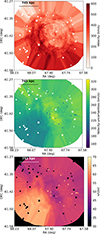 |
Fig. 6. Velocity maps for the A3266 cluster. Top panel: Velocity map (km/s) relative to the A3266 cluster (z = 0.0594). Maps were created by moving 2:1 elliptical regions (i.e., rotated to lie tangentially to the nucleus) containing ∼750 counts in the Fe-K region. Middle panel: 1σ velocity uncertainties. White circles correspond to point sources which were excluded from the analysis. The spectral fitting was done in the 4 − 9.25 keV energy range. Bottom panel: Significance of the velocity measurements (v/Δv). |
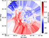 |
Fig. 7. Velocity map (km/s) relative to the A3266 cluster, taking as reference (i.e., zero level in the color scale) the mean value 312 km/s obtained from the spectral map described in Sect. 6. |
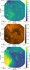 |
Fig. 8. Spectral maps of the A3266 cluster. Top panel: Temperature map in units of keV. Middle panel: Abundance map relative to abundances from Lodders et al. (2009). Bottom panel: Emission measure map. The spectral fitting was done in the 4 − 9.25 keV energy range. |
4.2. Velocity radial profiles
We proceeded to analyze annular regions to study the radial velocity structure. The thickness of these rings increases as the square root of the distance from the center of A3266. Figure 9 shows the exact spatial regions analyzed. Table 2 presents the best-fit results obtained for each region, numbered from the center outward, while Fig. 10 displays the resulting velocity structure. We achieved velocity measurements with an accuracy of up to  km/s (for ring 4). The largest redshift or blueshift relative to A3266 is (805 ± 284) km/s for ring 5. As is observed in the spectral map (see Sect. 4.1), we obtained a redshifted velocity distribution for almost all regions. For distances of less than 240 kpc, the velocities tend to increase with the radius. We found a mean velocity of ∼283 km/s for all regions. We computed a χ2 test based on the null hypothesis that the velocities are consistent with a constant velocity model and obtained a p-value =0.33. Thus, the observed variations in velocity are not due to random chance. Figure 11 shows the temperature (top panel) and metallicity (bottom panel) distribution. We found a uniform distribution for both parameters, similar to previous profiles computed by Ghirardini et al. (2019), Sanders et al. (2022). However, these values could be underestimated, since our spectral analysis does not include the soft energy band. Furthermore, the apparent correlation between the emission measure and metallicity is most likely an artifact, as the lower the metallicity, the larger the emission measure should be to obtain lines of comparable fluxes.
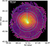 |
Fig. 9. A3266 annular regions analyzed in Sect. 4.2. Green circles correspond to point-like sources excluded from the analysis. |
A3266 cluster best-fit parameters for annular regions.
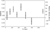 |
Fig. 10. Velocities obtained for each annular region described in Sect. 4.2 (numbered from the center to the outside). The A3266 redshift is indicated with a horizontal line. The spectral fitting was done in the 4 − 9.25 keV energy range. |
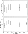 |
Fig. 11. Temperature (top panel) and metallicity (bottom panel) profiles obtained from the best-fit results for each annular region described in Sect. 4.2. The spectral fitting was done in the 4 − 9.25 keV energy range. |
4.3. Discontinuities in the surface-brightness
To study the velocity structure, we manually selected multiple regions based on the fractional difference in 0.5–2 keV X-ray surface brightness. The top panel of Fig. 12 shows the regions used for the analysis, similar to those identified in Sanders et al. (2022). The regions can be identified as follows: the central core (region 1), cavities (regions 2–4), the western structure (region 5), the northeastern structures (regions 6, 7), the bridge (region 8), and the northwestern structure (region 9). Table 3 shows the best-fit results. As is shown in the spectral map (see Sect. 4.1), we found redshifted velocities for all regions, with the largest velocities corresponding to cavity 2 ( km/s) and the northeastern structure (region 6,
  km/s). The velocities for the remaining structures were similar, considering the uncertainties.
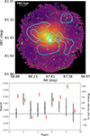 |
Fig. 12. Surface brightness maps of the A3266 cluster. Top panel: Manually selected regions following the fractional difference in 0.5–2 keV X-ray surface brightness. Green circles correspond to point-like sources excluded from the analysis. Bottom panel: Velocities obtained for manually selected regions following the A3266 merging structure. The A3266 redshift is indicated with a horizontal line. The spectral fitting was done in the 4 − 9.25 keV energy range. We have also included the mean optical redshift for galaxies from Dehghan et al. (2017) within each one of the regions obtained. |
A3266 cluster best-fit parameters for manually selected regions following the A3266 merging structure.
For each region identified in Sanders et al. (2022), we selected the galaxies within the region for which Dehghan et al. (2017) obtained optical redshifts. Then, we computed the mean optical redshift within each one of the regions (red points in Fig. 12). Table 3 also includes the mean optical redshift computed in this way. The mean galactic velocities are within the ICM velocities except for regions 1, 4, 7, and 8. The mean ICM velocity for all regions is ∼275 km/s and the mean galactic velocities are ∼525 km/s. However, the regions following the surface brightness discontinuities do not correspond to the substructures identified in Dehghan et al. (2017). Figure 13 shows the temperature (top panel) and metallicity (bottom panel) for these regions. Both parameters are uniform across the different regions, hinting at increasing metallicity in region 2.
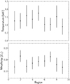 |
Fig. 13. Temperature (top panel) and metallicity (bottom panel) profiles obtained from the best-fit results for manually selected regions following the A3266 merging structure. The spectral fitting was done in the 4 − 9.25 keV energy range. |
4.4. Probability distribution function
Figure 14 shows the velocity PDF computed from the velocity map, weighted by area. We ran normality tests, including the Shapiro-Wilk (Shapiro & Wilk 1965, SHA+65) and D’Agostino and Pearson’s (D’Agostino & Pearson 1973, DAG+73), to determine if a Gaussian models the data well. The PDF follows a normal distribution as the p value is larger than the α = 0.05 level for both tests (0.63 for SHA+65 and 0.71 for DAG+73). The overall redshift obtained from the Gaussian fit is 314 ± 12 km/s with a velocity dispersion of σv = 67 ± 12 km/s.
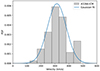 |
Fig. 14. Velocity PDF of the hot ICM obtained for the A3266 velocity map. The blue line corresponds to the best fit using a Gaussian model. |
Following Gatuzz et al. (2023b), we computed the first-order VSF by taking the weighted average of the difference between the line-of-sight velocities (v) of two points separated by r. However, due to large uncertainties, we only have estimated upper limits of < 600 km/s up to ∼3000 kpc scales.
5. Discussion
We have found that the ICM, on average, moves away from A3266 with velocities increasing from ∼300–800 km/s across the cluster (Fig. 6). After subtracting the cluster systemic redshift, a blueshifted-redshifted structure is observed around the cluster center (Fig. 7). However, no clear spiral pattern associated with gas sloshing is observed (as seen, for example, in Sanders et al. 2020). The blueshifted region also displays lower metallicity, which may indicate recent mixing or gas stripping in this area.
The velocity dispersions of the hot gas measured in this study (∼200–400 km/s) are consistent with simulations that predict a relatively isotropic velocity distribution in the hot ICM phase (Ayromlou et al. 2023), and they align with previous observations of other massive clusters. For example, for the Perseus cluster, Hitomi measured up to σv ∼ 220 km/s, while XMM-Newton measurements by Gatuzz et al. (2023b) reported dispersions of 344 ± 18 km/s in Virgo, 371 ± 12 km/s in Centaurus, and 847 ± 92 km/s in Ophiuchus. The upper limits we found for the VSF also agree with those computed for the Virgo, Centaurus, and Ophiuchus clusters (see Fig. 3 in Gatuzz et al. 2023b). We did not find hints of a multimodal PDF associated with merging events, compared, for example, with the Ophiuchus cluster (Gatuzz et al. 2023b).
The velocity structure of the ICM and galaxies in A3266 presents an interesting contrast, but direct comparisons between these two components must be treated with caution. Nevertheless, examining both provides insights into the overall cluster dynamics and the role of substructures in shaping these motions. Dehghan et al. (2017) measured an overall optical redshift for the cluster galaxies of ∼200 ± 50 km/s with respect to the cluster core, with a velocity dispersion of 1337 ± 67 km/s. This large dispersion reflects not virialized motions but rather the relative motions of substructures and infalling groups within the cluster, which have been studied. For example, the western core substructure has a redshift of ∼600 relative to the cluster center, while other subgroups have velocities of ∼559 km/s and ∼393 km/s (Dehghan et al. 2017, see their Table 3). These large velocities are primarily driven by substructure dynamics and merger activity rather than by processes affecting the ICM, such as shocks (Liu et al. 2015, 2016; Ota & Yoshida 2016; Liu et al. 2018).
We observe that the mean optical velocities for some substructures tend to be more than twice as large as the mean ICM velocities across the regions we examined (see Fig. 12). This discrepancy reflects the fact that the optical velocities are influenced by the motion of substructures and merging groups within the cluster. In contrast, the ICM velocities primarily trace the bulk motions of the gas. The optical velocity data from Dehghan et al. (2017) indicate the presence of infalling groups, which move at significantly higher velocities relative to the cluster core, while the ICM velocities, which are generally lower, likely reflect the slower response of the gas to the gravitational potential and interactions with the shock fronts. While these components exhibit different kinematic behavior, both point to a cluster that is not yet fully relaxed, with significant dynamical interactions shaping its velocity structure.
6. Conclusions and summary
We have analyzed the velocity structure of the hot ICM within the A3266 galaxy cluster. We measured line-of-sight velocities of the gas using the technique developed by Sanders et al. (2020), Gatuzz et al. (2022a,b), which allows a better calibration of the absolute energy scale of the XMM-Newton EPIC-pn detector. Our main findings and conclusions are:
-
1.
We studied the morphological structures within the galaxy cluster by applying a GGM and adaptively smoothed GGM filter to the EPIC-pn X-ray image.
-
2.
We made 2D projected maps for the velocity, temperature, and metallicity. We have found that the hot gas within the system displays a redshifted velocity with respect to the cluster redshift along all the fields of view. After subtracting the average redshift, the velocity spectral map does show an opposite blueshifted-redshifted structure, with the blueshifted region displaying a lower metallicity.
-
3.
We studied the velocity distribution by creating non-overlapping circular regions. Our results are consistent with redshifted velocities as far as 1125 kpc from the cluster core.
-
4.
We analyzed the velocity distribution along regions following the discontinuities in the surface brightness. We found redshifted velocities for all regions, with the largest velocities being 805 ± 284 km/s.
-
5.
We computed the velocity PDF from the velocity map. By applying a normality test, we found that the PDF follows an unimodal normal distribution, as was predicted by simulations.
-
6.
We obtained upper limits for the VSF of < 600 km/s up to ∼3000 kpc scales.
Finally, the present work will be followed by a detailed study of the temperature and abundance distribution by modeling the soft X-ray spectra of the A3266 galaxy cluster.
Acknowledgments
This work was supported by the Deutsche Zentrum für Luft- und Raumfahrt (DLR) under the Verbundforschung programme (Messung von Schwapp-, Verschmelzungs- und Rückkopplungsgeschwindigkeiten in Galaxienhaufen.). This work is based on observations obtained with XMM-Newton, an ESA science mission with instruments and contributions directly funded by ESA Member States and NASA. This research was carried out on the High Performance Computing resources of the raven cluster at the Max Planck Computing and Data Facility (MPCDF) in Garching operated by the Max Planck Society (MPG).
References
- Ahoranta, J., Finoguenov, A., Pinto, C., et al. 2016, A&A, 592, A145 [NASA ADS] [CrossRef] [EDP Sciences] [Google Scholar]
- Ascasibar, Y., & Markevitch, M. 2006, ApJ, 650, 102 [Google Scholar]
- Ayromlou, M., Nelson, D., & Pillepich, A. 2023, MNRAS, 524, 5391 [CrossRef] [Google Scholar]
- Cash, W. 1979, ApJ, 228, 939 [Google Scholar]
- D’Agostino, R., & Pearson, E. S. 1973, Biometrika, 60, 613 [Google Scholar]
- Dehghan, S., Johnston-Hollitt, M., Colless, M., & Miller, R. 2017, MNRAS, 468, 2645 [NASA ADS] [CrossRef] [Google Scholar]
- Dennerl, K., Andritschke, R., Bräuninger, H., et al. 2020, SPIE Conf. Ser., 11444, 114444Q [NASA ADS] [Google Scholar]
- Edge, A. C., Stewart, G. C., Fabian, A. C., & Arnaud, K. A. 1990, MNRAS, 245, 559 [NASA ADS] [Google Scholar]
- Ettori, S., Ghirardini, V., Eckert, D., et al. 2019, A&A, 621, A39 [NASA ADS] [CrossRef] [EDP Sciences] [Google Scholar]
- Fabian, A. C., Walker, S. A., Russell, H. R., et al. 2017, MNRAS, 464, L1 [NASA ADS] [CrossRef] [Google Scholar]
- Federrath, C., Roman-Duval, J., Klessen, R. S., Schmidt, W., & Mac Low, M. M. 2010, A&A, 512, A81 [NASA ADS] [CrossRef] [EDP Sciences] [Google Scholar]
- Federrath, C., Klessen, R. S., Iapichino, L., & Beattie, J. R. 2021, Nat. Astron., 5, 365 [NASA ADS] [CrossRef] [Google Scholar]
- Finoguenov, A., Henriksen, M. J., Miniati, F., Briel, U. G., & Jones, C. 2006, ApJ, 643, 790 [NASA ADS] [CrossRef] [Google Scholar]
- Foster, A., Smith, R., & Brickhouse, N. S. 2019, Am. Astron. Soc. Meet. Abstr., 233, 251.05 [NASA ADS] [Google Scholar]
- Gaspari, M., Churazov, E., Nagai, D., Lau, E. T., & Zhuravleva, I. 2014, A&A, 569, A67 [NASA ADS] [CrossRef] [EDP Sciences] [Google Scholar]
- Gatuzz, E., Sanders, J. S., Dennerl, K., et al. 2022a, MNRAS, 511, 4511 [NASA ADS] [CrossRef] [Google Scholar]
- Gatuzz, E., Sanders, J. S., Canning, R., et al. 2022b, MNRAS, 513, 1932 [NASA ADS] [CrossRef] [Google Scholar]
- Gatuzz, E., Sanders, J. S., Dennerl, K., et al. 2023a, MNRAS, 522, 2325 [NASA ADS] [CrossRef] [Google Scholar]
- Gatuzz, E., Mohapatra, R., Federrath, C., et al. 2023b, MNRAS, 524, 2945 [NASA ADS] [CrossRef] [Google Scholar]
- Gatuzz, E., Sanders, J. S., Dennerl, K., et al. 2023c, MNRAS, 520, 4793 [NASA ADS] [CrossRef] [Google Scholar]
- Gatuzz, E., Sanders, J. S., Dennerl, K., et al. 2023d, MNRAS, 525, 6394 [NASA ADS] [CrossRef] [Google Scholar]
- Gatuzz, E., Sanders, J. S., Dennerl, K., et al. 2023e, MNRAS, 526, 396 [NASA ADS] [CrossRef] [Google Scholar]
- Ghirardini, V., Eckert, D., Ettori, S., et al. 2019, A&A, 621, A41 [NASA ADS] [CrossRef] [EDP Sciences] [Google Scholar]
- Henriksen, M. J., & Tittley, E. R. 2002, ApJ, 577, 701 [NASA ADS] [CrossRef] [Google Scholar]
- Henriksen, M., Donnelly, R. H., & Davis, D. S. 2000, ApJ, 529, 692 [NASA ADS] [CrossRef] [Google Scholar]
- Hitomi Collaboration (Aharonian, F., et al.) 2016, Nature, 535, 117 [Google Scholar]
- Hitomi Collaboration (Aharonian, F., et al.) 2018, PASJ, 70, 12 [NASA ADS] [Google Scholar]
- Hofmann, F., Sanders, J. S., Nandra, K., Clerc, N., & Gaspari, M. 2016, A&A, 585, A130 [NASA ADS] [CrossRef] [EDP Sciences] [Google Scholar]
- Kalberla, P. M. W., Burton, W. B., Hartmann, D., et al. 2005, A&A, 440, 775 [NASA ADS] [CrossRef] [EDP Sciences] [Google Scholar]
- Lau, E. T., Kravtsov, A. V., & Nagai, D. 2009, ApJ, 705, 1129 [NASA ADS] [CrossRef] [Google Scholar]
- Liu, A., Yu, H., Tozzi, P., & Zhu, Z.-H. 2015, ApJ, 809, 27 [Google Scholar]
- Liu, A., Yu, H., Tozzi, P., & Zhu, Z.-H. 2016, ApJ, 821, 29 [Google Scholar]
- Liu, A., Yu, H., Diaferio, A., et al. 2018, ApJ, 863, 102 [NASA ADS] [CrossRef] [Google Scholar]
- Lodders, K., Palme, H., & Gail, H. P. 2009, Landolt Börnstein, 4B, 712 [Google Scholar]
- McNamara, B. R., & Nulsen, P. E. J. 2012, New J. Phys., 14, 055023 [NASA ADS] [CrossRef] [Google Scholar]
- Navarro, J. F., Frenk, C. S., & White, S. D. M. 1996, ApJ, 462, 563 [Google Scholar]
- Ota, N., & Yoshida, H. 2016, PASJ, 68, S19 [NASA ADS] [CrossRef] [Google Scholar]
- Pinto, C., Sanders, J. S., Werner, N., et al. 2015, A&A, 575, A38 [NASA ADS] [CrossRef] [EDP Sciences] [Google Scholar]
- Predehl, P., Andritschke, R., Arefiev, V., et al. 2021, A&A, 647, A1 [EDP Sciences] [Google Scholar]
- Sanders, J. S., Fabian, A. C., Russell, H. R., Walker, S. A., & Blundell, K. M. 2016a, MNRAS, 460, 1898 [Google Scholar]
- Sanders, J. S., Fabian, A. C., Taylor, G. B., et al. 2016b, MNRAS, 457, 82 [Google Scholar]
- Sanders, J. S., Dennerl, K., Russell, H. R., et al. 2020, A&A, 633, A42 [EDP Sciences] [Google Scholar]
- Sanders, J. S., Biffi, V., Brüggen, M., et al. 2022, A&A, 661, A36 [NASA ADS] [CrossRef] [EDP Sciences] [Google Scholar]
- Sauvageot, J. L., Belsole, E., & Pratt, G. W. 2005, A&A, 444, 673 [NASA ADS] [CrossRef] [EDP Sciences] [Google Scholar]
- Seta, A., Federrath, C., Livingston, J. D., & McClure-Griffiths, N. M. 2023, MNRAS, 518, 919 [Google Scholar]
- Shapiro, S. S., & Wilk, M. B. 1965, Biometrika, 52, 591 [Google Scholar]
- Simionescu, A., Werner, N., Finoguenov, A., Böhringer, H., & Brüggen, M. 2008, A&A, 482, 97 [NASA ADS] [CrossRef] [EDP Sciences] [Google Scholar]
- Strüder, L., Briel, U., Dennerl, K., et al. 2001, A&A, 365, L18 [Google Scholar]
- Tamura, T., Yamasaki, N. Y., Iizuka, R., et al. 2014, ApJ, 782, 38 [NASA ADS] [CrossRef] [Google Scholar]
- Wilms, J., Allen, A., & McCray, R. 2000, ApJ, 542, 914 [Google Scholar]
- Zhuravleva, I., Churazov, E., Schekochihin, A. A., et al. 2014, Nature, 515, 85 [Google Scholar]
- ZuHone, J. A., Miller, E. D., Simionescu, A., & Bautz, M. W. 2016, ApJ, 821, 6 [NASA ADS] [CrossRef] [Google Scholar]
- ZuHone, J. A., Miller, E. D., Bulbul, E., & Zhuravleva, I. 2018, ApJ, 853, 180 [NASA ADS] [CrossRef] [Google Scholar]
All Tables
A3266 cluster best-fit parameters for manually selected regions following the A3266 merging structure.
All Figures
|
Fig. 1. RGB and X-ray images of the A3266 cluster. Top panel: RGB image of A3266. The bands used are 0.2–0.5 keV (R), 0.5–1.0 keV (G), and 1.0–2.0 keV (B). We applied a σ = 1 Gaussian smoothing to the exposure-corrected and background-subtracted image. Bottom panel: Exposure-corrected and background-subtracted X-ray surface brightness of the A3266 cluster in the 0.5–9.25 keV energy range. The point-like sources were excluded in the analysis. The 10-level contours of the X-ray image are shown in white. |
| In the text | |
|
Fig. 2. Exposure maps and Fe, Cu counts map for the A3266 cluster. Top panel: Total exposure time (s) in the 0.5–9.25 keV energy range. Middle panel: Normalized Fe-K count map, showing the number of counts in each 1.59 arcsec pixel in the Fe-K complex with the instrumental Cu ring included to indicate the regions in which the redshift can be measured. Bottom panel: Normalized background Cu count map, showing the number of counts in each 1.59 arcsec pixel in the Cu Kα line energy range. |
| In the text | |
|
Fig. 3. Edge-filtered X-ray images using a Gaussian gradient magnitude (GGM) filter on scales of 4 pixels (top panel) and 8 pixels (bottom panel). |
| In the text | |
|
Fig. 4. Edge-filtered X-ray images using an adaptive Gaussian gradient magnitude (GGM) filter from Sanders et al. (2022) using a signal-to-noise ratio of 32, where the scale shows the gradient as the log(10) change per 4 arcsec pixel. |
| In the text | |
|
Fig. 5. Subtracted fractional difference from the average at each radius for the 0.5–2 keV X-ray surface brightness. The point-like sources were excluded in the analysis. The X-ray image was smoothed by a 2σ Gaussian. |
| In the text | |
|
Fig. 6. Velocity maps for the A3266 cluster. Top panel: Velocity map (km/s) relative to the A3266 cluster (z = 0.0594). Maps were created by moving 2:1 elliptical regions (i.e., rotated to lie tangentially to the nucleus) containing ∼750 counts in the Fe-K region. Middle panel: 1σ velocity uncertainties. White circles correspond to point sources which were excluded from the analysis. The spectral fitting was done in the 4 − 9.25 keV energy range. Bottom panel: Significance of the velocity measurements (v/Δv). |
| In the text | |
|
Fig. 7. Velocity map (km/s) relative to the A3266 cluster, taking as reference (i.e., zero level in the color scale) the mean value 312 km/s obtained from the spectral map described in Sect. 6. |
| In the text | |
|
Fig. 8. Spectral maps of the A3266 cluster. Top panel: Temperature map in units of keV. Middle panel: Abundance map relative to abundances from Lodders et al. (2009). Bottom panel: Emission measure map. The spectral fitting was done in the 4 − 9.25 keV energy range. |
| In the text | |
|
Fig. 9. A3266 annular regions analyzed in Sect. 4.2. Green circles correspond to point-like sources excluded from the analysis. |
| In the text | |
|
Fig. 10. Velocities obtained for each annular region described in Sect. 4.2 (numbered from the center to the outside). The A3266 redshift is indicated with a horizontal line. The spectral fitting was done in the 4 − 9.25 keV energy range. |
| In the text | |
|
Fig. 11. Temperature (top panel) and metallicity (bottom panel) profiles obtained from the best-fit results for each annular region described in Sect. 4.2. The spectral fitting was done in the 4 − 9.25 keV energy range. |
| In the text | |
|
Fig. 12. Surface brightness maps of the A3266 cluster. Top panel: Manually selected regions following the fractional difference in 0.5–2 keV X-ray surface brightness. Green circles correspond to point-like sources excluded from the analysis. Bottom panel: Velocities obtained for manually selected regions following the A3266 merging structure. The A3266 redshift is indicated with a horizontal line. The spectral fitting was done in the 4 − 9.25 keV energy range. We have also included the mean optical redshift for galaxies from Dehghan et al. (2017) within each one of the regions obtained. |
| In the text | |
|
Fig. 13. Temperature (top panel) and metallicity (bottom panel) profiles obtained from the best-fit results for manually selected regions following the A3266 merging structure. The spectral fitting was done in the 4 − 9.25 keV energy range. |
| In the text | |
|
Fig. 14. Velocity PDF of the hot ICM obtained for the A3266 velocity map. The blue line corresponds to the best fit using a Gaussian model. |
| In the text | |
Current usage metrics show cumulative count of Article Views (full-text article views including HTML views, PDF and ePub downloads, according to the available data) and Abstracts Views on Vision4Press platform.
Data correspond to usage on the plateform after 2015. The current usage metrics is available 48-96 hours after online publication and is updated daily on week days.
Initial download of the metrics may take a while.