| Issue |
A&A
Volume 692, December 2024
|
|
|---|---|---|
| Article Number | A65 | |
| Number of page(s) | 16 | |
| Section | Interstellar and circumstellar matter | |
| DOI | https://doi.org/10.1051/0004-6361/202451499 | |
| Published online | 03 December 2024 | |
The SOFIA Massive (SOMA) Star Formation Q-band follow-up
I. Carbon-chain chemistry of intermediate-mass protostars
1
National Astronomical Observatory of Japan, National Institutes of Natural Sciences,
2-21-1 Osawa, Mitaka,
Tokyo
181-8588,
Japan
2
Rosseland Centre for Solar Physics, University of Oslo,
PO Box 1029
Blindern,
0315
Oslo,
Norway
3
Institute of Theoretical Astrophysics, University of Oslo,
PO Box 1029
Blindern,
0315
Oslo,
Norway
4
Department of Astronomy, University of Virginia,
Charlottesville,
VA
22904,
USA
5
Department of Space, Earth & Environment, Chalmers University of Technology,
412 93
Gothenburg,
Sweden
6
Observatorio Astronomico Nacional (OAN-IGN),
Alfonso XII 3,
28014
Madrid,
Apain
7
Instituto de Astrofísica de Andalucía, CSIC,
Glorieta de la Astronomía s/n,
18008
Granada,
Spain
8
Star and Planet Formation Laboratory, RIKEN Cluster for Pioneering Research,
Wako, Saitama
351-0198,
Japan
9
National Radio Astronomy Observatory,
520 Edgemont Rd.,
Charlottesville,
VA
22903,
USA
10
Department of Earth and Planetary Sciences, Institute of Science Tokyo,
Meguro, Tokyo
152-8551,
Japan
11
Graduate Institute for Advanced Studies,
SOKENDAI, 2-21-1 Osawa,
Mitaka, Tokyo
181-8588,
Japan
12
Department of Astronomy, Shanghai Jiao Tong University,
800 Dongchuan Rd., Minhang,
Shanghai
200240,
PR China
13
Green Bank Observatory,
155 Observatory Rd,
Green Bank,
WV
24944,
USA
14
European Southern Observatory,
Karl-Schwarzschild-Str. 285748 Garching bei,
München,
Germany
15
Osservatorio Astrofisico di Arcetri,
Largo Enrico Fermi, 5,
50125
Firenze FI,
Italy
★ Corresponding author; kotomi.taniguchi@nao.ac.jp
Received:
14
July
2024
Accepted:
24
October
2024
Context. Evidence that the chemical characteristics around low- and high-mass protostars are similar has been found: notably, a variety of carbon-chain species and complex organic molecules (COMs) form around both types. On the other hand, the chemical compositions around intermediate-mass (IM) protostars (2 M⊙ < m* < 8 M⊙) have not been studied with large samples. In particular, it is unclear the extent to which carbon-chain species form around them.
Aims. We aim to obtain the chemical compositions of a sample of IM protostars, focusing particularly on carbon-chain species. We also aim to derive the rotational temperatures of HC5N to confirm whether carbon-chain species are formed in the warm gas around these stars.
Methods. We conducted Q-band (31.5–50 GHz) line survey observations toward 11 mainly IM protostars with the Yebes 40 m radio telescope. The target protostars were selected from a subsample of the source list of the SOFIA Massive Star Formation project. Assuming local thermodynamic equilibrium, we derived the column densities of the detected molecules and the rotational temperatures of HC5N and CH3 OH.
Results. Nine carbon-chain species (HC3N, HC5N, C3H, C4H linear-H2CCC, cyclic-C3H2, CCS, C3S, and CH3CCH), three COMs (CH3OH, CH3CHO, and CH3CN), H2CCO, HNCO, and four simple sulfur-bearing species (13CS, C34S, HCS+, and H2CS) are detected. The rotational temperatures of HC5N are derived to be ~20–30 K in three IM protostars (Cepheus E, HH288, and IRAS 20293+3952). The rotational temperatures of CH3OH are derived in five IM sources and found to be similar to those of HC5N.
Conclusions. The rotational temperatures of HC5N around the three IM protostars are very similar to those around low- and high-mass protostars. These results indicate that carbon-chain molecules are formed in lukewarm gas (~20–30 K) around IM protostars via the warm carbon-chain chemistry process. Thus, carbon-chain formation occurs ubiquitously in the warm gas around protostars across a wide range of stellar masses. Carbon-chain molecules and COMs coexist around most of the target IM protostars, which is similar to the situation for low- and high-mass protostars. In summary, the chemical characteristics around protostars are the same in the low-, intermediate- and high-mass regimes.
Key words: astrochemistry / stars: formation
© The Authors 2024
 Open Access article, published by EDP Sciences, under the terms of the Creative Commons Attribution License (https://creativecommons.org/licenses/by/4.0), which permits unrestricted use, distribution, and reproduction in any medium, provided the original work is properly cited.
This article is published in open access under the Subscribe to Open model. Subscribe to A&A to support open access publication.
1 Introduction
Many astrochemical studies have been dedicated to investigating the chemical compositions around protostars (for a review, see Jørgensen et al. 2020). It is well known that complex organic molecules (COMs), which consist of more than six atoms (Herbst & van Dishoeck 2009), are abundant in hot regions with temperatures ≥100 K, namely hot cores and hot corinos around high-mass (m* ≥ 8 M⊙) and low-mass (m* ≤ 2 M⊙) protostars, respectively. These COMs are formed on dust surfaces during the cold pre-stellar core stage and/or the warm-up stage after protostars are born, or they are synthesized in hot gas around protostars (e.g., Skouteris et al. 2019; Jin & Garrod 2020; Garrod et al. 2022).
Sakai et al. (2008) detected high-excitation lines of carbon-chain species, such as cyclic-C3H2, linear-C3H2, C4H, C4H2, and CH3CCH, from the low-mass protostar L1527. Sakai et al. (2010) found that the intensity distribution of cyclic-C3H2 shows a steep increase within 500–1000 au of the protostar. At these distances, temperatures range from ≈20–30 K. These carbon-chain species are not a remnant of the parent molecular cloud but instead formed from CH4 sublimated from dust grains at around 25 K (Hassel et al. 2008). This carbon-chain formation pro-cess was named warm carbon-chain chemistry (WCCC; Sakai et al. 2008). Oya et al. (2017) show that carbon-chain species and COMs coexist around the low-mass protostar L483, but their spatial distributions are different; COMs are concentrated in the central hot corino regions, whereas carbon-chain species are more extended and absent at the central protostar position. This type of source is called a hybrid.
This chemical diversity around low-mass protostars may be caused by the different strengths of the interstellar radiation field (ISRF), as proposed by Spezzano et al. (2017) based on their observations toward the pre-stellar core L1544. Subsequent single-dish survey observations detected the presence of carbon-chain species and/or COMs across various low-mass pro-tostars, including hot corinos, WCCC sources, and hybrid-type sources. Lefloch et al. (2018) find that carbon-chain-rich sources are located on the outsides of dense filaments, whereas hot-corino type sources are mainly present inside the dense filament, which is shielded from the ISRF. These results, which are consis-tent with the scenario proposed by Spezzano et al. (2017), were interpreted as follows: the CO molecules, precursors of COMs, can survive in the dense regions and COMs become abundant, whereas CO is destroyed by the ISRF in the less shielded regions. The destruction of CO leads to high abundances of C and C+, precursors of carbon-chain species, outside the dense filament or at the edge of the molecular clouds, and these conditions are favorable for the formation of WCCC-type sources. Therefore, a pre-stellar environment could significantly modify the chemistry in the protostellar envelope, potentially promoting the formation of carbon-chain molecules with higher C abundances.
Studies on the carbon-chain species of high-mass protostars followed. Green et al. (2014) conducted survey observations of the HC5N (J = 12−11) line toward 79 high-mass protostars associated with the 6.7 GHz methanol masers. They detected the HC5N line from 35 sources. After these survey observations, follow-up observations were conducted. Taniguchi et al. (2017) derived the abundances of HC5N toward three high-mass proto-stars and conclude that these abundances cannot be explained by the WCCC mechanism. Taniguchi et al. (2019a) show that the observed abundance ratio of HC5N/CH3OH around the high-mass protostar G28.28−0.36 (Taniguchi et al. 2018a) can be reproduced in their hot-core model when the temperature reaches 100 K. More recently, Taniguchi et al. (2023) presented spatial distributions of carbon-chain species (HC3N, HC5N, and CCH) and COMs toward five high-mass protostars obtained with the Atacama Large Millimeter/submillimeter Array (ALMA) Band 3, and indicated that HC5N exists in the hot-core regions where the temperature is above 100 K. Based on these findings, they proposed hot carbon-chain chemistry (HCCC) to explain the observational results around high-mass protostars. In the HCCC mechanism, carbon-chain species are formed in the warm gas, adsorbed onto dust grains, and accumulated in ice mantles below 100 K, and these carbon-chain species evaporate into the gas phase when the temperature reaches 100 K. Stable carbon-chain species such as cyanopolyynes (HC2n+1N, n = 1,2,3,…) are more abundant than unstable radical-type carbon-chain species (e.g., CCH and CCS) in HCCC compared to WCCC (for a review, see Taniguchi et al. 2024a).
Although astrochemical studies toward low-mass and high-mass protostars have become more common, our knowledge about the chemical compositions around intermediate-mass (IM) protostars (2 M⊙ < m* < 8 M⊙) remains limited. Alonso-Albi et al. (2010) investigated the CO depletion and N2H+ deuteration toward Class 0 IM protostars with the IRAM 30 m telescope. They were able to fit the C18O (J = 1−0) maps assuming that the C18O abundance decreases inward within the protostellar envelope until the temperatures of the gas and dust reach ≈20–25 K, corresponding to the sublimation temperature of CO. The deuterium fractionation of N2H+ was found to be 0.005–0.014, which is lower than those in pre-stellar clumps by a factor of 10. The chemical compositions of COMs have only been investigated toward a few IM protostars. Fuente et al. (2014) observed the IM protostar NGC 7129 FIRS 2 with the IRAM Plateau de Bure Interferometer (PdBI) and IRAM 30 m telescope, and detected numerous COMs (e.g., CH3OCHO, CH3CH2OH, CH2OHCHO, aGg’-(CH2OH)2, and CH3CH2CN) from its central hot region. They find similarities between the chemical compositions of this IM protostar and that of the Orion KL hot core, suggesting that the IM protostar NGC 7129 FIRS 2 contains a hot core. Lines of COMs have been detected from another IM protostar, Cepheus E (Ospina-Zamudio et al. 2018). Ospina-Zamudio et al. (2018) observed this source with the IRAM 30 m telescope and the NOrthern Extended Millimeter Array (NOEMA) and detected various COMs, including large species such as CH3COCH3 and C2H5CN.
Although it has been shown that hot corino chemistry emerges around IM protostars, it is still unclear whether carbon-chain molecules are formed in warm and/or hot regions (i.e., whether WCCC and/or HCCC proceed) and whether chemical diversity emerges as well as in low-mass and high-mass regimes. To address these questions, we need observations of carbon-chain species around IM protostars and an investigation of their abundances relative to COMs.
This paper presents Q-band (31.5–50 GHz) line survey observations toward 11 mainly IM protostars with the Yebes 40 m telescope. We focus on carbon-chain molecules, whose rota-tional transition lines can be efficiently observed in the Q band. We aim to determine whether carbon-chain molecules are formed in warm gas around IM protostars. Modeling of the struc-ture of IM protostellar envelopes by Crimier et al. (2010) shows that the radius of the 30 K dust and gas region is approximately 0.01–0.02 pc.
The paper is organized as follows. Section 2 explains details of the observations with the Yebes 40 m telescope. The results and spectral analyses are presented in Sects. 3.1 and 3.2, respec-tively. We discuss carbon-chain chemistry and the chemical characteristics around IM protostars by comparing them with low-mass and high-mass regimes in Sect. 4. Our main conclu-sions are summarized in Sect. 5.
2 Observations
We carried out Q-band (31.5–50 GHz) line survey observations with the Yebes 40 m radio telescope (Proposal IDs 22A008 and 22B005, PI Kotomi Taniguchi). Eleven target protostars were selected from a subsample of the source list of the SOFIA Massive (SOMA) Star Formation project (De Buizer et al. 2017; Liu et al. 2020) based on the following criteria: (1) the source declination is above +20°, and (2) other infrared sources are not contaminated within the Yebes beam size (≈40″–50″).
Table 1 summarizes the details of target sources. The coordinates correspond to the beam center of our observations. We list the protostellar properties derived by Fedriani et al. (2023) from spectral energy distribution (SED) fitting. We note that Lbol is the intrinsic bolometric luminosity of the source, which can be different from the luminosity inferred from the received bolo-metric flux assuming isotropic emission (Lbol,iso) that is often quoted in observational studies of the protostars. This is because the received bolometric flux is affected by the orientation of the protostar (i.e., the "flashlight effect") and by foreground extinction.
The subsample mainly consists of IM protostars, and the central values of available stellar masses (m*) are within the IM regime (Table 1). However, we note that IRAS 23385+6053 has previously been categorized as a high-mass protostar (Beuther et al. 2023). In the end, our target source list consists of 10 IM protostars and 1 high-mass source (IRAS 23385+6053). We abbreviate IRAS source names as I plus the first five numbers before "+" in the rest of this paper (e.g., 100420). Five sources (Cepheus E, L1206, HH288, 100420, and 120434) were observed in the 22A008 program, and the other seven sources were observed in the 22B005 program. The observations were carried out February 5–14, 2022 (22A008) and between September 2022 and January 2023 (22B005).
We employed the standard position-switching mode. The off-source positions were regions where the visual extinction (AV) is below 3 mag in the Av maps obtained from the Atlas and Catalogue of Dark Clouds (Dobashi et al. 2005)1.
The Q-band receiver, one of the Nanocosmos receivers (Tercero et al. 2021), was used for the observations. This receiver obtains dual-polarization (H and V) data. The fast Fourier trans-form spectrometers with 38 kHz resolution and 2.5 GHz band-width mode were used. Eight base bands were allocated for each polarization, and the 31.5–50 GHz band was observed simul-taneously. The frequency resolution of 38 kHz corresponds to ~0.3 km s−1 in the Q band. The main beam efficiencies (ηMB) and beam sizes (the half-power beam width) were approximately 50– 65% and 36″–54″, respectively, between 32 GHz and 49 GHz. The calibration was performed at the beginning of the position-switching, observing the sky and both hot and cold loads; this procedure was repeated every 18 min. Pointing and focus were corrected every hour based on pseudo-continuum observations of intense SiO maser lines toward evolved stars close to our target sources. The pointing errors were within 7″ and the calibration uncertainties are estimated to be less than 15%. The obtained antenna temperature  was converted to the main beam temperature (TMB) using the following formula (Tercero et al. 2021):
  ·, where ηF is the forward efficiency (0.91–0.93 in the Q band; Tercero et al. 2021).
Summary of the 11 target sources.
3 Results and analyses
3.1 Results
We made fits files of the spectra from CLASS (software from the GILDAS package), and further data reduction was con-ducted with the CASSIS software (Vastel et al. 2015). Spec-tra of carbon-chain species (HC3N, HC5N, C3H, linear (l)-H2CCC, cyclic (c)-C3H2, C4H, CCS, C3S, and CH3CCH), COMs (CH3OH, CH3CHO, and CH3CN), H2CCO, HNCO, and sulfur-bearing species (13CS, C34S, HCS+, and H2CS) toward the 11 sources are available on Zenodo. We categorized CCS and C3S into carbon-chain species following the definitions provided in Taniguchi et al. (2024a) even though they contain a sulfur atom. Table A.1 summarizes the information on each line (tran-sition, rest frequency, and upper-state energy). The average rms noise levels measured in line-free channels are around 5 mK.
Table 2 summarizes the detection status in each source. Cyanoacetylene (HC3N) is detected from all of the sources, and cyanodiacetylene (HC5N) is detected from all of the sources except 105380 and 121307. c-C3H2 is associated with the pro-tostars where HC5N has been detected. Two c-C3H2 lines show different features, which are likely caused by different upper-state energies (Table A.1). CCS is detected from all of the sources except for I 21307. All of the carbon-chain species listed in Table 2 are detected from L1206, HH288, and 122198. All the other sources except I 05380 and I 21307 show lines from at least five carbon-chain species. Only three and two carbon-chain species from I 05380 and I 21307 are detected.
In addition to carbon-chain species, three COMs (CH3OH, CH3CHO, and CH3CN), H2CCO, and HNCO are detected in the Q band. Methanol (CH3OH), one of the most fundamental COMs, and S-bearing species are detected from all of the sources except I 05380. We can see the wing emission in the spectra of CH3OH in Cepheus E, I 00259, and I 20293. Except for these three sources, the 41,4 – 30,3 E lines of CH3OH show a single peak and the line peak coincides with the rest frequency, which means that the emission comes from low-velocity quiescent gas, presumably envelopes.
The IM protostars L1206, HH288, and I 22198 are the most line-rich sources, whereas I 05380 is likely a line-poor source. The source distance of I 05380 is 1.34 kpc (Table 1), and this source is not the farthest one, which means that the beam dilu-tion effect (a beam size of ≈40″ corresponds to 0.25 pc at 1.34 kpc) is not responsible for the non-detection of molecular lines. This source has the lowest luminosity among our target IM protostars, and the gas and dust temperatures could be lower. Thus, the hot and warm regions are smaller than those of the other sources. These physical conditions may have limited our species detections.
Detection status in IM protostars.
3.2 Spectral analyses
We derived rotational temperatures using seven HC5N lines (from J = 12–11 to J = 18–17) and four CH3OH lines in the Q band (Sect. 3.2.1). The rotational temperature provides a hint of where carbon-chain species exist: outer cold envelopes, luke-warm envelopes, or central hot-core regions. Such a distinction is important for constraining the formation processes of carbon-chain species around IM protostars (i.e., are they just a remnant of the parent molecular cloud or a product of WCCC or HCCC) (Taniguchi et al. 2024a). We analyzed spectra and derived the column densities of the other species with the Markov chain Monte Carlo (MCMC) method assuming local thermodynamic equilibrium (LTE) because there is not enough data to conduct the rotational diagram analysis (Sect. 3.2.2).
3.2.1 Rotational diagram of HC5N and CH3OH
We fitted the spectra with a Gaussian profile and conducted rotational diagram analysis using the CASSIS software (Vastel et al. 2015). We applied this method to all of the sources where the HC5 N lines have been detected. However, we were only able to fit the data and derive rotational temperatures for three sources, Cepheus E, HH288, and I 20293. We could not derive the rota-tional temperatures in the other sources because the data points cannot be fitted using this method. This is likely caused by low signal-to-noise ratios (S/Ns) of the lines and/or non-Gaussian profiles.
The top panels of Fig. 1 show the rotational diagrams of HC5N in these three sources. The J = 12–11 line shows systematically lower values in all of the sources and could not be fitted with the other lines simultaneously. This is caused by the fact that the lowest J line was observed at the edge of the band of the receiver, and some systematic effects caused the intensity fluctuation. In addition, it is likely that HC5N is located in both cold envelopes and warm envelopes; contributions from cold envelopes are larger for the lowest energy line. Since its spatial distributions are unknown, we cannot estimate the beam dilution effect for each line. Thus, we could not correct the beam-filling factors, so we derived the average rotational temperatures within the beams. We need observations of lower J lines to cover cold-envelope components.
We fitted the data excluding the J = 12–11 line to avoid the systematic effects mentioned in the preceding paragraph. The rotational temperatures were derived to be 20.0 ± 2.5 K, 17.3 ± 2.7 K, and 29.3 ± 14.3 K in Cepheus E, HH288, and I 20293, respectively. The rotational temperatures in Cepheus E and HH288 are well constrained, and we used these temperatures in the analyses of the other carbon-chain species (Sect. 3.2.2).
We conducted rotational diagram analysis for the CH3OH data. The spectra in several sources show non-Gaussian profiles, such as wing emission or complicated several-velocity compo-nents, and we could not obtain rotational temperatures in these cases. We were able to use this method for the five sources that show Gaussian profiles. The middle and bottom panels of Fig. 1 show the rotational diagrams of these five sources. The derived rotational temperatures of CH3OH are around 20–30 K, which are similar to those of HC5N. Since the observed lines of CH3OH have low upper-state energies (Table A.1) and the line widths are relatively narrow, the emission likely comes from low-velocity quiescent gas in the envelope (Taniguchi et al. 2020; Tychoniec et al. 2021; Gorai et al. 2024).
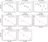 |
Fig. 1 Rotational diagrams of HC5N and CH3OH. 10% errors are indicated for each data point. |
3.2.2 Markov chain Monte Carlo method
We conducted MCMC spectral analysis using the CASSIS software (Vastel et al. 2015). We assumed LTE for all of the species. In the fitting procedure, we treated the molecular column density (N), line width (the full width at half maximum), and centroid velocity (VLSR) as free parameters. Since we do not know the molecular spatial distributions, we derived the beam-averaged column densities.
In analyses of carbon-chain species (except for HC5N and CH3CCH), we fixed the excitation temperatures (Tex) because we could not determine both the column density and the exci-tation temperature simultaneously due to insufficient lines. The excitation temperature of 20 K was used for all of the sources except for HH288, for which we used the rotational tempera-ture of HC5N (17.3 K; Sect. 3.2.1). We could not fit all of the lines of CCS, c-C3H2, and l-H2CCC simultaneously under the assumption of a single excitation temperature of 20 K. In that case, we divided the spectra into two groups based on the upper-state energies; lines with low upper-state energies (Eup/k ≤ 9 K) were fitted with an excitation temperature of 10 K, whereas those with high upper-state energies (Eup /k ≥ 12 K) were fitted with an excitation temperature of 20 K. We indicate these dif-ferent assumed excitation temperatures as "(low)" and "(high)," respectively, in Table A.2. The assumed excitation temperature of 10 K is a typical gas kinetic temperature for starless cores. Such a method was applied because we assumed that carbon-chain molecules are present in both the outer cold envelopes and the warm envelopes, which are close to the IM protostars.
We tentatively detect l-H2C3 in Cepheus E, and we treated its column density as the upper limit. We fitted four C4H lines simultaneously because they have similar upper-state energies. We did not fit lines with non-Gaussian profiles or low S/Ns. However, all of the lines cannot be well fitted simultaneously: the fit of the N = 5–4 line emission fails to reproduce the N = 4–3 line emission, and vice versa. Only the best-fitting results that show the smallest chi-square values are displayed in the spectral figures. However, the derived physical parameters were calcu-lated taking this issue into account; large errors are included in the derived physical parameters if all of the lines were not fitted simultaneously.
In the case of HC5N, we treated the excitation temperature as an additional free parameter because its seven lines are available, which means that its column densities and excitation tempera-tures were determined simultaneously. In I 00259 and I 23385, the S/Ns are not high enough or several lines were not detected, and so we fixed the excitation temperature at 20 K. We could not fit the J = 12–11 line with the other lines simultaneously due to systematically low intensities (see also Sect. 3.2.1). We therefore fitted the J = 12–11 transition with a fixed excitation temperature of 10 K, but the column densities derived by this line should be considered reference values due to the uncertainties in peak intensities. In Table A.2, these column densities are labeled "(low)." The other lines were fitted with the excitation tempera-ture as a free parameter. The determined excitation temperatures and column densities are listed in Tables 3 and A.2, respectively.
We derived the column densities and excitation temperatures of CH3CCH using two K-ladder lines (K = 0 and 1) with the MCMC method for the five sources. The rotational temperatures are derived to be around 20 K, which are consistent with those of HC5N (Table 3). These results provide evidence that carbon-chain species exist in warm regions because the abundance of CH3CCH is suggested to be increased by the WCCC mechanism (Taniguchi et al. 2019a).
In our analyses of COMs and S-bearing species, we used an excitation temperature of 20 K, which is constrained by the rota-tional diagram analyses of CH3OH (Sect. 3.2.1). We treated the excitation temperature as a free parameter of the CH3OH data in I 21307 and I 22198, in which two lines with a Gaussian profile (41,4 − 3−0,3 E and 10,1 − 00,0 A) have been detected. The derived excitation temperatures are summarized in Table 3. For 123385, the excitation temperature was fixed to 20 K. We excluded spectra with low S/Ns and non-Gaussian profiles from the fitting. We analyzed spectra with the two velocity components for CH3CN in I 20293, and 13CS, C34S, and H2CS in I 23385. The two veloc-ity components in I 23385 are consistent with those found in the C18O and C17O lines (−50.5 km s−1 and −47.8 km s−1; Fontani et al. 2004). Although CH3CN has two K-ladder lines, the K = 1 line was detected with low S/Ns and we could not use it for the fitting. We thus fitted the K = 0 line with a fixed excitation temperature in the CH3CN analysis.
The derived column densities are summarized in Table A.2. Some column densities show large uncertainties due to low S/Ns or non-Gaussian line features. The derived line widths and centroid velocities are summarized in Table A.3.
Excitation temperatures of HC5N, CH3OH, and CH3CCH derived via the MCMC method.
4 Discussion
4.1 Comparison of the rotational temperatures of HC5N
Here we compare the rotational temperatures of HC5N around IM protostars to those around low-mass and high-mass counter-parts. We utilize the results obtained by single-dish telescopes, and the derived rotational temperatures are beam-averaged values.
Sakai et al. (2009) carried out the Q-band observations with the Green Bank 100 m Telescope (GBT) and 3 mm band (90– 150 GHz) observations with the IRAM 30 m telescope toward the low-mass protostar L1527 (d = 140 pc), which is one of the WCCC sources (Sakai et al. 2008). They derived a rotational temperature for HC5N of 14.7 ± 5.3 K using three lines (J = 16– 15, 17–16, and 32–31). We note that the rotational temperature was derived by fitting with almost two data points because the upper-state energies of the J = 16–15 and J = 17–16 transitions are similar.
Taniguchi et al. (2017) detected the HC5N lines in the Ka band (J = 10–9 and 11–10) with GBT, and in the 45 GHz (J = 16–15 and 17–16) and 90 GHz (J = 31–30, 32–31, 34–33, 36–35, 38–37, and 39–38) bands with the Nobeyama 45 m radio telescope from three high-mass protostars, which are also mas-sive young stellar objects (MYSOs; G 12.89+0.49, G 16.86–2.16, and G 28.28–0.36). The rotational temperatures with the beam-size correction are 18 ± 2,17 ± 2, and  K in G 12.89+0.49 (d = 2.94 kpc), G 16.86-2.16 (d = 1.7 kpc), and G28.28-0.36 (d = 3.0 kpc), respectively. Because the observations have a low angular resolution, these temperatures are considered to be lower limits due to contamination from outer cold envelopes, as pointed out by Taniguchi et al. (2021).
In the case of the IM protostars, the rotational temperatures of HC5N were derived to be around 20 K (Sect. 3.2.1). In the MCMC analysis, the derived excitation temperatures are slightly higher (~25 K) but consistent with the former within the errors. The rotational temperatures around the IM protostars are close to those around the low-mass and high-mass protostars and clearly higher than the gas kinetic temperature in molecular clouds (~ 10 K). In addition, the excitation temperatures around the IM protostars agree with the WCCC scenario in which CH4 sublimated from dust grains around 25 K forms carbon-chain species. These results imply that carbon-chain molecules are formed in warm gas around IM protostars by WCCC (Sakai et al. 2008; Hassel et al. 2008) or HCCC (Taniguchi et al. 2019a, 2023). The derived excitation temperatures of CH3CCH also support this scenario.
Here, we constrain which mechanism is dominant in our observations, WCCC or HCCC. The size of the hot region of Cepheus E, with temperatures above 100 K, was estimated to be 0.7″, corresponding to ~510 au (Ospina-Zamudio et al. 2018). Thus, our target sources should have much smaller hot regions (T > 100 K) compared to the beam size (40″–50″). This means that the detected carbon-chain emission around the IM protostars should come from warm envelopes rather than central hot regions. Thus, we conclude that the WCCC mech-anism forms the carbon-chain species around the IM protostars. We need high-angular-resolution (≤0.5″) observations to inves-tigate whether the HCCC mechanism works around the IM protostars.
Since our observations only cover lines with upper-state energies around 10–22 K (Table A.1), the detected emission may be biased to warm or cold components (i.e., the outer layers of the protostellar envelopes). Even in this case, our conclusion that carbon-chain species form around the IM protostars is robust. Since the photodissociation region (PDR) chemistry does not produce HC5N efficiently, the detected emission of HC5N likely comes from mainly warm central gas, not the cavity walls of molecular outflows.
In summary, the carbon-chain formation around protostars occurs ubiquitously. It is difficult to conclude which formation mechanism is dominant, WCCC or HCCC, around IM protostars from the rotational temperatures derived using Q-band single-dish observations. We need high J transition observations and imaging observations with interferometers to resolve the current open questions.
4.2 Comparison of the chemical compositions
Figure 2 compares the molecular abundances with respect to HC3N, which are defined as N(molecules)/N(HC3N), of the 11 protostars. We used HC3N as the standard because it has been detected in all the sources, and it is useful for comparisons to results in low-mass and high-mass regimes, as we describe later. The various panels show comparisons of carbon-chain species, three COMs, H2CCO, HNCO, and S-bearing species. If two velocity components have been derived, we plotted the sums of the two.
As a general trend, the derived abundances do not vary among the sources when we focus on a particular molecule, especially the S-bearing species. On the other hand, the abun-dances of CH3OH vary more significantly for I 21307, I 22198, and I 23385, which have larger abundances compared to the other sources whose abundances we were able to derive. The fact that we can see wing emission in their spectra means that the CH3OH lines come not only from warm envelopes but also from molecular outflows and shock regions, as noted in Sect. 3.2.1.
We compared the abundances with respect to HC3N of the 11 protostars and the low-mass WCCC source L1527 (Yoshida et al. 2019). The C4H/HC3N ratio in L1527 was derived to be ~19, which is higher than those of our target sources. The high-temperature components of HC5N in Cepheus E, L1206, and I 22198 show similar values as L1527 (~0.2), whereas HH288, I 00420, I 20343, I 00259, I 20293, and I 23385 show slightly lower values than L1527. The abundances of c-C3H2 around the IM protostars tend to be lower than that of L1527 (≈3.6). The abundances of the other carbon-chain species in IM protostars are consistent with those of L1527 within the errors; the abundance ratios in L1527 are CCS/HC3N≈0.49, l-H2CCC/HC3N≈0.1, and CH3CCH/HC3N≈5.7. These results suggest that the formation of large carbon-chain species has not yet occurred around most of the target IM protostars, because the WCCC mechanism starts with CH4 and small carbon-chain species form first.
The CH3OH/HC3N ratio in L1527 is around 1.9, which is close to those of L1206, HH288, and I 20343 and lower than those of I 21307, I 22198, and I 23385. On the other hand, the CH3CN/HC3N ratios of all of the IM protostars are higher than that of L1527 (~0.02), which is expected because L1527 is deficient in COMs. Hence, the N-bearing COM is more abun-dant around the IM protostars than the low-mass WCCC source, whereas the CH3OH abundances seem to depend on the source properties.
The chemical characteristics of the IM protostars can be summarized as follows:
The compositions of small carbon-chain species are similar to those in L1527;
The abundances of larger carbon-chain species tend to be low compared to L1527;
Three IM protostars (L1206, HH288, and 120343) have similar CH3OH/HC3N abundance ratios as L1527, whereas two IM sources (I 21307 and I 22198) have much higher ratios; this implies that the CH3OH abundances depend on the source characteristics;
CH3CN is more abundant around the IM protostar than around L1527.
Next, we compared the HC5N/HC3N abundance ratios to those in high-mass protostellar objects (HMPOs) derived from Q-band observations with the Nobeyama 45 m radio telescope (Taniguchi et al. 2018b). We calculated the HC5N/HC3N toward 14 HMPOs where both species have been detected (Taniguchi et al. 2018b). The average HC5N/HC3N ratio is 0.3, but there is a large scatter, from 0.1 to 1.0. The HC5N/HC3N ratios in the IM protostars are similar to the minimum and average values of HMPOs.
We obtained the HC5N/HC3N and CH3OH/HC3N abundance ratios toward three MYSOs (G 12.89+0.49, G 16.86-2.16, and G 28.28-0.36) from Taniguchi et al. (2018a). These three MYSOs are more physically evolved than HMPOs. At the MYSO stage, the HCCC mechanism produces cyanopolyynes efficiently (Taniguchi et al. 2023). The MYSO G 12.89+0.49 is found to be a COM-rich hot core, whereas G 28.28-0.36 is a carbon-chain-rich and COM-poor source. The HC5N/HC3N ratios are 0.2 toward G 12.89+0.49 and G 16.86-2.16, and 0.3 toward G28.28-0.36. The HC5N/HC3N abundance ratios around the IM protostars are consistent with or slightly lower than those of the MYSOs.
The CH3OH/HC3N ratios are 21, 12, and 3 in the three MYSOs G 12.89+0.49, G 16.86-2.16, and G 28.28-0.36, respec-tively. The ratio in I 00420 is consistent with those in G 12.89+0.49 and G 16.86-2.16 within the errors, whereas the ratios for L1206, HH288, and I 20343 match with that for G28.28-0.36. The ratios for I22198 and I21307 are higher than that for G 12.89+0.49 by a factor of approximately 3 and 7, respectively.
In summary, the HC5N/HC3N ratios in the IM protostars are close to those in HMPOs and MYSOs in single-dish scales.
Since we used results obtained by the single-dish telescopes, their emission is dominated by warm envelopes rather than the hot-core regions. The WCCC mechanism works ubiquitously around protostars of various stellar masses and produces similar chemical compositions of carbon-chain species.
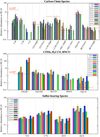 |
Fig. 2 Comparison of molecular abundances with respect to HC3N for: carbon-chain species (top), COMs, H2CCO, and HNCO (middle), and S-bearing species (bottom). Errors indicate the standard deviation. In the caption, "high" and "low" indicate the high and low temperatures components. The dashed red lines mark the abundance ratios for the low-mass WCCC source L1527 (Yoshida et al. 2019). |
4.3 Relationship between bolometric luminosity and the HC5N/HC3N abundance ratio
Energetic particles such as UV radiation and cosmic rays could increase the HC5N/HC3N ratios (Fontani et al. 2017; Taniguchi et al. 2019a). For instance, Fontani et al. (2017) find that the emission of HC3N and HC5N does not coincide in OMC2-FIR4; HC3N emission overlaps relatively well with the continuum emission, whereas HC5N emits only in the eastern half. In this subsection we investigate a possible correlation between the bolometric luminosity and the HC5N/HC3N abundance ratio based on data toward low-mass, IM, and high-mass protostars.
Figure 3 shows the relationship between the HC5N/HC3N abundance ratios and the source bolometric luminosity. We plot data toward IM protostars, the low-mass WCCC source L1527 (Yoshida et al. 2019), HMPOs (Taniguchi et al. 2018b), and the MYSO G 12.89+0.49 (Taniguchi et al. 2018a) to cover a wide range of bolometric luminosity. No correlation is found between the bolometric luminosity and the HC5N/HC3N ratio. This implies that the formation of cyanopolyynes around protostars is not dominated by UV radiation and energetic particles. This ensures that the WCCC mechanism, which depends only on the temperature, forms carbon-chain species.
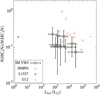 |
Fig. 3 HC5N/HC3N column density ratio vs. bolometric luminosity toward various protostars. The column densities were derived using single-dish observations. Information on the bolometric luminosities of L1527, HMPOs, and G12 are taken from Shirley et al. (2002), Sridharan et al. (2002), and Taniguchi et al. (2023), respectively. |
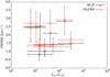 |
Fig. 4 Line widths of HC5N (black) and CH3CHO (red) vs. bolometric luminosity. |
4.4 Comparison of line widths and centroid velocities
The line width and centroid velocity provide a clue as to what each molecular line traces. In this subsection we compare these values for each source.
Figure A.1 shows comparison of the line width (full width at half maximum) obtained by the MCMC analyses (Sect. 3.2.2) of the different molecular lines for each IM protostar. We do not see any differences between carbon-chain species, COMs, H2CCO, HNCO, and S-bearing species. This suggests that both carbon-chain species and COMs possibly trace similar regions around the IM protostars (i.e., warm envelopes).
In Cepheus E, the lines of HC3N, the low upper-state-energy lines of CCS and l-H2CCC, and C34S show narrower line widths compared to the other lines. We can see similar trends in HC3N and C34S toward L1206 and the low upper-state-energy line of CCS in HH288. These lines likely trace mainly cold envelopes. However, these trends are not universal for all of the IM protostars. The different linear-scale beam sizes (≈0.14–1.0 pc) – in other words, different source distances (≈0.7–5 kpc; see Table 1) – may affect these results.
Figure A.2 compares the centroid velocity (VLSR) of each molecular line obtained via the MCMC analyses (Sect. 3.2.2). All of the lines have values similar to the source systemic velocities in Cepheus E, I 00420, I 20343, I 20293, I 21307, and I 22198. The velocities of the molecular lines in HH288, except for c-C3H2, are slightly higher than the source systemic velocity. The velocities of all of the molecular lines seem to be higher than the systemic source velocity in L1206. This could happen because the source velocity in L1206 was derived by the maser. The thermal molecular lines likely have different velocity components than the maser lines.
We can see velocity shifts in the molecular lines from the source systemic velocities in L1206, HH288, and I 23385. There are no available data for the systemic velocities of I 00259 and I 05380. Here, we provide systemic velocities of these protostars based on the results of HC3N, which is a good dense core tracer: −10 km s−1 for L1206, −28.5 km s−1 for HH288, −39 km s−1 for I 00259, 2.5 km s−1 for 105380, and −50.3 km s−1 for I 23385. Table A.3 summarizes this information.
For the CH3CN in I 20293 and the 13CS and C34S in I 23385, two velocity components were identified. The two velocity components of CH3CN in I 20293 are different from those of the other lines, but the lower velocity component is marginally consistent with that of HCS+ within the errors. We cannot identify the cause(s) of the velocity shifts in the single-dish observations. In the case of the isotopomers of CS in I 23385, the low-velocity components (−50 km s−1) are similar to most of the other molecular lines, whereas the high-velocity component is similar to those of C4H and the high-velocity component of CCS (low). As seen in Fig. A.1, the C4H lines in I 23385 show wider line features (~3.6 km s−1) than the other sources. Hence, the emission region of C4H in I 23385 may be different from that of the other IM protostars; for example, it could be the cavity wall of the molecular outflows. Such a difference suggests that I 23385 contains a more massive star than IM protostars and that the powerful outflow(s) affect the spatial distributions of these molecules, which agrees with the conclusions of Beuther et al. (2023).
Figure 4 shows a plot of line widths of HC5N (black) and CH3CHO (red) versus the bolometric luminosity. There is no correlation between the bolometric luminosity and line widths of either species in the bolometric luminosity range of the target IM protostars. These results imply that the observed lines trace regions less affected by the central stars; the lack of correlation is caused by the low-angular-resolution data obtained by the single-dish telescope. Similarly, no correlations between the bolometric luminosity and line widths of carbon-chain species were found toward the HMPOs observed with the Nobeyama 45 m telescope (Taniguchi et al. 2019b).
4.5 The cyclic-to-linear ratio of the C3H2 isomer
We investigated the cyclic-to-linear ratios (hereafter the c/l ratios) by combining observations and theoretical studies (Sipilä et al. 2016; Loison et al. 2017). Physical conditions likely affect the c/l ratios. For instance, the c/l ratios of C3H2 were found to be 110 ± 30 and 30 ± 10 for molecular clouds with densities of 104 cm−3 and 4 × 105 cm−3, respectively (Loison et al. 2017). The c/l ratio at the starless clump in the Serpens South cluster-forming region was derived to be 58 ± 6 (Taniguchi et al. 2024b). These results imply that the density plays a key role in producing differences in the c/l ratio of the C3H2 isomers. It has been proposed that isomerization reactions of l-C3 H2 + H → c-C3 H2 + H and t-C3H2 + H → c-C3H2 + H are responsible for the high c/l ratio in low-density conditions (Loison et al. 2017). In this subsection we compare the c/l ratio of the C3H2 isomers of the IM protostars.
Figure 5 shows a comparison of the c/l ratios of the C3H2 isomers, c-C3H2 and l-H2CCC. "Low" (blue) and "high" (red) mean that the ratios were derived using the low Eup lines assuming an excitation temperature of 10 K and the high Eup lines assuming an excitation temperature of 20 K, respectively (see Sect. 3.2). Since l-H2CCC has been tentatively detected in Cepheus E and I 00259 and their column densities are the upper limits, their c/l ratios are the lower limits. The spectra of c-C3H2 show weak peak intensities in I 00420, and the relative error is large. If we exclude the three sources with large uncertainties, the low components have a c/l ratio in the range 10–20. The low components have higher ratios than the high components (~3−5) in the three sources for which both of the components have been detected, albeit with large errors.
This may reflect the fact that outer cold envelopes (the low component) have lower densities than inner warm regions, where the WCCC mechanism occurs (the high component). However, the temperature may also affect the c/l ratio. Since previous the-oretical studies did not take the warm-up phase into account, this remains unclear.
The c/l ratio in the WCCC source is lower than those in the cold pre-stellar cores; the c/l ratios in pre-stellar cores were derived to be ~30−110 (Sipilä et al. 2016; Loison et al. 2017), whereas the ratio in L1527 was derived to be 12 (Sipilä et al. 2016). This tendency is visible Fig. 5: the low components have higher values than the high components. These two different c/ l ratios support the scenario that carbon-chain species exist in both the outer, less dense envelopes and the inner, denser envelopes.
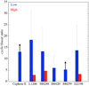 |
Fig. 5 Cylic-to-linear ratios of the C3H2 isomers c-C3H2 and l-H2CCC. The blue and red bars indicate the ratios for the low- and high-temperature components as a function of the upper-state energies (see Sect. 3.2.2). |
4.6 Carbon and sulfur isotopic ratios in CS
Figure 6 compares the C34S/13 CS abundance ratios of the ten protostars. Comp 1 and Comp 2 of I 23385 mean two different velocity components; −50 km s−1 and −47.8 km s−1, respectively.
The local interstellar medium (ISM) value (2.8 ± 0.6; Yan et al. 2023) was calculated using the following formula and adopting the results of the CS isotopologs:
 (1)
(1)
The observed ratios are consistent with the local ISM value within the errors. Comp 2 of I 23385, whose velocity component is VLSR ≈ −47.8 km s−1, has a higher C34S/13CS abundance ratio than the local ISM. Since I 23385 has the highest bolometric luminosity and is a high-mass protostar, one possible explana-tion for such an isotope anomaly is that the local UV radiation destroys less-abundant isotopologues (13CS) more efficiently (i.e., the self-shielding effect). Or, the PDR-like chemistry at the cavity wall of the molecular outflow may affect the chemistry of Comp 2. Three outflows or jets have been identified in this high-mass protostellar system via several shock tracers, including SiO, H2, [Fe II], and [Ne II] (Beuther et al. 2023). If Comp 2 traces the outflow components, the self-shielding effect may be responsible for the high C34S/13CS ratio only in Comp 2. High-angular-resolution observations that resolve the two differ-ent components are needed to determine the origin of the isotope anomaly.
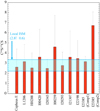 |
Fig. 6 C34S/13CS ratios for the ten IM protostars. The Comp 1 and Comp 2 of I 23385 are −50 km s−1 and −47.8 km s−1, respectively. The local ISM value (2.8 ± 0.6) was calculated from the results of Yan et al. (2023). |
5 Conclusions
We conducted Q-band line survey observations toward 11 pro-tostars, which were selected from the subsample source list of the SOMA project, with the Yebes 40 m telescope. The main findings and conclusions of this paper are as follows:
We have detected nine carbon-chain species (HC3N, HC5N, C3H, C4H, linear-H2CCC, cyclic-C3H2, CCS, C3S, and CH3CCH), three COMs (CH3OH, CH3CHO, and CH3CN), H2CCO, HNCO, and four S-bearing species (13CS, C34S, HCS+,and H2CS);
The derived rotational temperatures of HC5N are approximately 20–30 K, suggesting that carbon-chain molecules exist in warm regions around the IM protostars. The rota-tional temperatures are consistent with those derived in low-mass and high-mass protostars. We need to observe high J lines to confirm the presence of hot components;
Based on comparisons of the chemical compositions around the IM protostars to those in the low-mass WCCC source L1527, HMPOs, and MYSO, the HC5N/HC3N ratios are found to be similar to those around low-mass and high-mass protostars. Since the beam size of the single-dish telescope is much larger than the hot regions around IM protostars, the detected carbon-chain emission must come from warm envelopes where the WCCC mechanism is dominant. To confirm the HCCC mechanism, we need interferometric observations to obtain their spatial distributions;
No correlations are found between the bolometric luminosity and the HC5N/HC3 N abundance ratio and line width. This implies that these cyanopolyynes are not formed by the PDR chemistry and supports the WCCC scenario;
The c/l ratios of the C3H2 isomers suggest that these species exist in regions with at least two different physical condi-tions: the less dense outer regions and denser inner regions. These results support our assumption that carbon-chain species exist in outer cold envelopes too;
The C34S/13CS ratios in the IM protostars generally agree with the value in the local ISM. However, the second veloc-ity component in I 23385 (~−47 km s−1) has a higher ratio. Since this is a high-mass protostar with a high bolomet-ric luminosity, the enhancement of the local UV radiation may produce such an isotopic anomaly. Or, the PDR-like chemistry at the cavity wall may affect it.
Our results confirm that carbon-chain species form in warm gas around IM protostars and that the WCCC mechanism is robust here. Future interferometric observations and higher-frequency line survey observations are needed to further constrain the chemical compositions and carbon-chain formation mechanisms around IM protostars, that is, to confirm the HCCC mechanism and compare the spatial distributions of carbon-chain species and COMs.
Data availability
The spectral figures are available on Zenodo (https://zenodo.org/records/13990455).
A copy of the reduced spectra is available at the CDS via anonymous ftp to cdsarc.cds.unistra.fr (130.79.128.5) or via https://cdsarc.cds.unistra.fr/viz-bin/cat/J/A+A/692/A65.
Acknowledgements
We deeply appreciate the staff of the Radiotelescope Administration of the Yebes Observatory (RYAO). K.T. is supported by JSPS KAK-ENHI grant Nos. JP20K14523, 21H01142, 24K17096, and 24H00252. This work was supported in part by Japan Foundation for Promotion of Astronomy. JCT acknowledges support from ERC Advanced Grant 788829 (MSTAR). M.G.-G. is partially supported by the research grant Nebulaeweb/ eVeNts (PID2019-105203GB-C21) of the Spanish AEI(MICIU). R.F. acknowledges support from the grants Juan de la Cierva FJC2021-046802-I, PID2020-114461GB-I00, PID2023-146295NB-I00, and CEX2021-001131-S funded by MCIN/AEI/ 10.13039/501100011033 and by "European Union NextGenerationEU/PRTR". Y.-L.Y. acknowledges support from Grant-in-Aid from the Ministry of Educa-tion, Culture, Sports, Science, and Technology of Japan (20H05845, 20H05844, 22K20389), and a pioneering project in RIKEN (Evolution of Matter in the Universe). We thank the anonymous referee whose comments helped improve the paper.
Appendix A Spectral line information and derived parameters
Information on the detected lines is summarized in Table A.1. Table A.2 summarizes the derived column densities for each source (Sect. 3.2). Table A.3 summarizes the line width (full width at half maximum) and the velocity component (VLSR) obtained via the MCMC analysis. Figure A.1 shows compari-son of line width (full width at half maximum) obtained via the MCMC analyses (Sect. 3.2.2) among different molecular lines for each IM protostar. Figure A.2 indicates comparison of the centroid velocity (VLSR) of each molecular line obtained via the MCMC analyses (Sect. 3.2.2).
Information on molecular lines.
Column densities.
Line widths and centroid velocity.
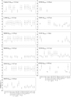 |
Fig. A.1 Comparison of line width (full width at half maximum) obtained via the MCMC analyses. θbeam indicates the linear-scale beam sizes of 40" at each source distance. |
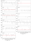 |
Fig. A.2 Comparison of the centroid velocity (VLSR) obtained via the MCMC analyses. The error bars do not include the velocity resolution of spectra (≈0.3 km s−1). The dashed gray horizontal lines indicate the systemic velocity of the source (Table 1). The dashed red horizontal lines indicate the systemic velocity updated or reported based on our results. |
References
- Alonso-Albi, T., Fuente, A., Crimier, N., et al. 2010, A&A, 518, A52 [NASA ADS] [CrossRef] [EDP Sciences] [Google Scholar]
- Beuther, H., van Dishoeck, E. F., Tychoniec, L., et al. 2023, A&A, 673, A121 [NASA ADS] [CrossRef] [EDP Sciences] [Google Scholar]
- Cesaroni, R., Beuther, H., Ahmadi, A., et al. 2019, A&A, 627, A68 [EDP Sciences] [Google Scholar]
- Crimier, N., Ceccarelli, C., Alonso-Albi, T., et al. 2010, A&A, 516, A102 [NASA ADS] [CrossRef] [EDP Sciences] [Google Scholar]
- de A Schutzer, A., Rivera-Ortiz, P. R., Lefloch, B., et al. 2022, A&A, 662, A104 [NASA ADS] [CrossRef] [EDP Sciences] [Google Scholar]
- De Buizer, J. M., Liu, M., Tan, J. C., et al. 2017, ApJ, 843, 33 [Google Scholar]
- Dobashi, K., Uehara, H., Kandori, R., et al. 2005, PASJ, 57, S1 [Google Scholar]
- Endres, C. P., Schlemmer, S., Schilke, P., Stutzki, J., & Müller, H. S. P. 2016, J. Mol. Spectrosc., 327, 95 [NASA ADS] [CrossRef] [Google Scholar]
- Fedriani, R., Tan, J. C., Telkamp, Z., et al. 2023, ApJ, 942, 7 [NASA ADS] [CrossRef] [Google Scholar]
- Fiorellino, E., Tychoniec, L., Cruz-Sáenz de Miera, F., et al. 2023, ApJ, 944, 135 [NASA ADS] [CrossRef] [Google Scholar]
- Fontani, F., Cesaroni, R., Testi, L., et al. 2004, A&A, 414, 299 [NASA ADS] [CrossRef] [EDP Sciences] [Google Scholar]
- Fontani, F., Ceccarelli, C., Favre, C., et al. 2017, A&A, 605, A57 [NASA ADS] [CrossRef] [EDP Sciences] [Google Scholar]
- Fuente, A., Cernicharo, J., Caselli, P., et al. 2014, A&A, 568, A65 [NASA ADS] [CrossRef] [EDP Sciences] [Google Scholar]
- Garrod, R. T., Jin, M., Matis, K. A., et al. 2022, ApJS, 259, 1 [NASA ADS] [CrossRef] [Google Scholar]
- Gorai, P., Law, C.-Y., Tan, J. C., et al. 2024, ApJ, 960, 127 [NASA ADS] [CrossRef] [Google Scholar]
- Green, C. E., Green, J. A., Burton, M. G., et al. 2014, MNRAS, 443, 2252 [NASA ADS] [CrossRef] [Google Scholar]
- Gueth, F., Schilke, P., & McCaughrean, M. J. 2001, A&A, 375, 1018 [NASA ADS] [CrossRef] [EDP Sciences] [Google Scholar]
- Hassel, G. E., Herbst, E., & Garrod, R. T. 2008, ApJ, 681, 1385 [Google Scholar]
- Herbst, E., & van Dishoeck, E. F. 2009, ARA&A, 47, 427 [NASA ADS] [CrossRef] [Google Scholar]
- Jin, M., & Garrod, R. T. 2020, ApJS, 249, 26 [Google Scholar]
- Jørgensen, J. K., Belloche, A., & Garrod, R. T. 2020, ARA&A, 58, 727 [Google Scholar]
- Karnath, N., Prchlik, J. J., Gutermuth, R. A., et al. 2019, ApJ, 871, 46 [NASA ADS] [CrossRef] [Google Scholar]
- Lefloch, B., Bachiller, R., Ceccarelli, C., et al. 2018, MNRAS, 477, 4792 [Google Scholar]
- Liu, M., Tan, J. C., De Buizer, J. M., et al. 2020, ApJ, 904, 75 [NASA ADS] [CrossRef] [Google Scholar]
- Loison, J.-C., Agúndez, M., Wakelam, V., et al. 2017, MNRAS, 470, 4075 [Google Scholar]
- Lundquist, M. J., Kobulnicky, H. A., Alexander, M. J., Kerton, C. R., & Arvidsson, K. 2014, ApJ, 784, 111 [CrossRef] [Google Scholar]
- Molinari, S., Testi, L., Brand, J., Cesaroni, R., & Palla, F. 1998, ApJ, 505, L39 [NASA ADS] [CrossRef] [Google Scholar]
- Ospina-Zamudio, J., Lefloch, B., Ceccarelli, C., et al. 2018, A&A, 618, A145 [NASA ADS] [CrossRef] [EDP Sciences] [Google Scholar]
- Oya, Y., Sakai, N., Watanabe, Y., et al. 2017, ApJ, 837, 174 [Google Scholar]
- Palau, A., Estalella, R., Ho, P. T. P., Beuther, H., & Beltrán, M. T. 2007, A&A, 474, 911 [NASA ADS] [CrossRef] [EDP Sciences] [Google Scholar]
- Pickett, H. M., Poynter, R. L., Cohen, E. A., et al. 1998, J. Quant. Spec. Radiat. Transf., 60, 883 [Google Scholar]
- Sakai, N., Sakai, T., Hirota, T., & Yamamoto, S. 2008, ApJ, 672, 371 [Google Scholar]
- Sakai, N., Sakai, T., Hirota, T., & Yamamoto, S. 2009, ApJ, 702, 1025 [Google Scholar]
- Sakai, N., Sakai, T., Hirota, T., & Yamamoto, S. 2010, ApJ, 722, 1633 [Google Scholar]
- Sánchez-Monge, Á., Palau, A., Estalella, R., et al. 2010, ApJ, 721, L107 [CrossRef] [Google Scholar]
- Shirley, Y. L., Evans, Neal J., I., & Rawlings, J. M. C. 2002, ApJ, 575, 337 [NASA ADS] [CrossRef] [Google Scholar]
- Sipilä, O., Spezzano, S., & Caselli, P. 2016, A&A, 591, L1 [NASA ADS] [CrossRef] [EDP Sciences] [Google Scholar]
- Skouteris, D., Balucani, N., Ceccarelli, C., et al. 2019, MNRAS, 482, 3567 [CrossRef] [Google Scholar]
- Spezzano, S., Caselli, P., Bizzocchi, L., Giuliano, B. M., & Lattanzi, V. 2017, A&A, 606, A82 [NASA ADS] [CrossRef] [EDP Sciences] [Google Scholar]
- Sridharan, T. K., Beuther, H., Schilke, P., Menten, K. M., & Wyrowski, F. 2002, ApJ, 566, 931 [Google Scholar]
- Sugitani, K., Fukui, Y., Mizuni, A., & Ohashi, N. 1989, ApJ, 342, L87 [NASA ADS] [CrossRef] [Google Scholar]
- Taniguchi, K., Saito, M., Hirota, T., et al. 2017, ApJ, 844, 68 [NASA ADS] [CrossRef] [Google Scholar]
- Taniguchi, K., Saito, M., Majumdar, L., et al. 2018a, ApJ, 866, 150 [NASA ADS] [CrossRef] [Google Scholar]
- Taniguchi, K., Saito, M., Sridharan, T. K., & Minamidani, T. 2018b, ApJ, 854, 133 [NASA ADS] [CrossRef] [Google Scholar]
- Taniguchi, K., Herbst, E., Caselli, P., et al. 2019a, ApJ, 881, 57 [Google Scholar]
- Taniguchi, K., Saito, M., Sridharan, T. K., & Minamidani, T. 2019b, ApJ, 872, 154 [Google Scholar]
- Taniguchi, K., Plunkett, A., Herbst, E., et al. 2020, MNRAS, 493, 2395 [NASA ADS] [CrossRef] [Google Scholar]
- Taniguchi, K., Herbst, E., Majumdar, L., et al. 2021, ApJ, 908, 100 [NASA ADS] [CrossRef] [Google Scholar]
- Taniguchi, K., Majumdar, L., Caselli, P., et al. 2023, ApJS, 267, 4 [CrossRef] [Google Scholar]
- Taniguchi, K., Gorai, P., & Tan, J. C. 2024a, Ap&SS, 369, 34 [NASA ADS] [CrossRef] [Google Scholar]
- Taniguchi, K., Nakamura, F., Liu, S.-Y., et al. 2024b, PASJ, accepted [arXiv:2409.16492] [Google Scholar]
- Tercero, F., López-Pérez, J. A., Gallego, J. D., et al. 2021, A&A, 645, A37 [EDP Sciences] [Google Scholar]
- Tychoniec, L., van Dishoeck, E. F., van’t Hoff, M. L. R., et al. 2021, A&A, 655, A65 [NASA ADS] [CrossRef] [EDP Sciences] [Google Scholar]
- Vastel, C., Bottinelli, S., Caux, E., Glorian, J. M., & Boiziot, M. 2015, in SF2A-2015: Proceedings of the Annual meeting of the French Society of Astronomy and Astrophysics, 313 [Google Scholar]
- Xu, Y., Voronkov, M. A., Pandian, J. D., et al. 2009, A&A, 507, 1117 [NASA ADS] [CrossRef] [EDP Sciences] [Google Scholar]
- Yan, Y. T., Henkel, C., Kobayashi, C., et al. 2023, A&A, 670, A98 [NASA ADS] [CrossRef] [EDP Sciences] [Google Scholar]
- Yoshida, K., Sakai, N., Nishimura, Y., et al. 2019, PASJ, 71, S18 [NASA ADS] [CrossRef] [Google Scholar]
All Tables
All Figures
|
Fig. 1 Rotational diagrams of HC5N and CH3OH. 10% errors are indicated for each data point. |
| In the text | |
|
Fig. 2 Comparison of molecular abundances with respect to HC3N for: carbon-chain species (top), COMs, H2CCO, and HNCO (middle), and S-bearing species (bottom). Errors indicate the standard deviation. In the caption, "high" and "low" indicate the high and low temperatures components. The dashed red lines mark the abundance ratios for the low-mass WCCC source L1527 (Yoshida et al. 2019). |
| In the text | |
|
Fig. 3 HC5N/HC3N column density ratio vs. bolometric luminosity toward various protostars. The column densities were derived using single-dish observations. Information on the bolometric luminosities of L1527, HMPOs, and G12 are taken from Shirley et al. (2002), Sridharan et al. (2002), and Taniguchi et al. (2023), respectively. |
| In the text | |
|
Fig. 4 Line widths of HC5N (black) and CH3CHO (red) vs. bolometric luminosity. |
| In the text | |
|
Fig. 5 Cylic-to-linear ratios of the C3H2 isomers c-C3H2 and l-H2CCC. The blue and red bars indicate the ratios for the low- and high-temperature components as a function of the upper-state energies (see Sect. 3.2.2). |
| In the text | |
|
Fig. 6 C34S/13CS ratios for the ten IM protostars. The Comp 1 and Comp 2 of I 23385 are −50 km s−1 and −47.8 km s−1, respectively. The local ISM value (2.8 ± 0.6) was calculated from the results of Yan et al. (2023). |
| In the text | |
|
Fig. A.1 Comparison of line width (full width at half maximum) obtained via the MCMC analyses. θbeam indicates the linear-scale beam sizes of 40" at each source distance. |
| In the text | |
|
Fig. A.2 Comparison of the centroid velocity (VLSR) obtained via the MCMC analyses. The error bars do not include the velocity resolution of spectra (≈0.3 km s−1). The dashed gray horizontal lines indicate the systemic velocity of the source (Table 1). The dashed red horizontal lines indicate the systemic velocity updated or reported based on our results. |
| In the text | |
Current usage metrics show cumulative count of Article Views (full-text article views including HTML views, PDF and ePub downloads, according to the available data) and Abstracts Views on Vision4Press platform.
Data correspond to usage on the plateform after 2015. The current usage metrics is available 48-96 hours after online publication and is updated daily on week days.
Initial download of the metrics may take a while.