| Issue |
A&A
Volume 692, December 2024
|
|
|---|---|---|
| Article Number | A138 | |
| Number of page(s) | 13 | |
| Section | Astrophysical processes | |
| DOI | https://doi.org/10.1051/0004-6361/202450836 | |
| Published online | 06 December 2024 | |
The CARMENES search for exoplanets around M dwarfs
The impact of rotation and magnetic fields on the radial velocity jitter in cool stars
1
Institut für Astrophysik und Geophysik, Georg-August-Universität, Friedrich-Hund-Platz 1, D-37077 Göttingen, Germany
2
Centre for Earth Evolution and Dynamics, Department of Geosciences, Universitetet i Oslo, Sem Sælands vei 2b, 0315 Oslo, Norway
3
Centro de Astrobiología (CSIC-INTA), Campus ESAC, Camino Bajo del Castillo s/n, 28692 Villanueva de la Cañada, Madrid, Spain
4
Max Planck Institute for Solar System Research, Justus-von-Liebig-Weg 3, 37077 Göttingen, Germany
5
Department of Physics, Ariel University, Ariel 40700, Israel
6
Instituto de Astrofśica de Canarias (IAC), 38200 La Laguna, Tenerife, Spain
7
Departamento de Astrofísica, Universidad de La Laguna, 38206 La Laguna, Tenerife, Spain
8
Instituto de Astrofísica de Andalucía (IAA-CSIC), Glorieta de la Astronomía s/n, 18008 Granada, Spain
9
Landessternwarte, Zentrum für Astronomie der Universität Heidelberg, Königstuhl 12, 69117 Heidelberg, Germany
10
Institut de Ciències de l’Espai (ICE, CSIC), Campus UAB, c/ Can Magrans s/n, E-08193 Bellaterra, Barcelona, Spain
11
Institut d’Estudis Espacials de Catalunya (IEEC), c/ Gran Capità 2-4, E-08034 Barcelona, Spain
12
Centro Astronónomico Hispano en Andalucía, Observatorio de Calar Alto, Sierra de los Filabres, 04550 Gérgal, Almería, Spain
13
Thüringer Landessternwarte Tautenburg, Sternwarte 5, 07778 Tautenburg, Germany
14
Max-Planck-Institut für Astronomie, Königstuhl 17, 69117 Heidelberg, Germany
15
Departamento de Física de la Tierra y Astrofísica and IPARCOS-UCM (Instituto de Física de Partículas y del Cosmos de la UCM), Facultad de Ciencias Físicas, Universidad Complutense de Madrid, 28040 Madrid, Spain
16
Hamburger Sternwarte, Universität Hamburg, Gojenbergsweg 112, 21029 Hamburg, Germany
⋆ Corresponding author; This email address is being protected from spambots. You need JavaScript enabled to view it.
Received:
22
May
2024
Accepted:
30
September
2024
Abstract
Context. Radial velocity (RV) jitter represents an intrinsic limitation on the precision of Doppler searches for exoplanets that can originate from both instrumental and astrophysical sources.
Aims. We aim to determine the RV jitter floor in M dwarfs and investigate the stellar properties that lead to RV jitter induced by stellar activity.
Methods. We determined the RV jitter in 239 M dwarfs from the CARMENES survey that are predominantly of mid to late spectral type and solar metallicity. We also investigated the correlation between stellar rotation and magnetic fields with RV jitter.
Results. The median jitter in the CARMENES sample is 3.1 m s−1, and it is 2.3 m s−1 for stars with an upper limit of 2 km s−1 on their projected rotation velocities. We provide a relation between the stellar equatorial rotation velocity and RV jitter in M dwarfs based on a subsample of 129 well-characterized CARMENES stars. RV jitter induced by stellar rotation dominates for stars with equatorial rotation velocities greater than 1 km s−1. A jitter floor of 2 m s−1 dominates in stars with equatorial rotation velocities below 1 km s−1. This jitter floor likely contains contributions from stellar jitter, instrumental jitter, and undetected companions. We study the impact of the average magnetic field and the distributions of magnetic filling factors on the RV jitter. We find a series of stars with excess RV jitter and distinctive distributions of magnetic filling factors. These stars are characterized by a dominant magnetic field component between 2 to 4 kG.
Conclusions. An RV jitter floor can be distinguished from RV jitter induced by activity and rotation based on the stellar equatorial rotation velocity. RV jitter induced by activity and rotation primarily depends on the equatorial rotation velocity. This RV jitter is also related to the distribution of magnetic filling factors, and this emphasizes the role of the magnetic field in the generation of RV jitter.
Key words: techniques: radial velocities / stars: activity / stars: low-mass / stars: magnetic field / stars: rotation
© The Authors 2024
 Open Access article, published by EDP Sciences, under the terms of the Creative Commons Attribution License (https://creativecommons.org/licenses/by/4.0), which permits unrestricted use, distribution, and reproduction in any medium, provided the original work is properly cited.
This article is published in open access under the Subscribe to Open model. This email address is being protected from spambots. You need JavaScript enabled to view it. to support open access publication.
1. Introduction
High-precision radial velocity (RV) searches of extrasolar planets often target low-mass stars, where it is possible to detect low-mass rocky planets (e.g. Zechmeister et al. 2019; Ribas et al. 2023) because the planet-to-star mass ratio is favorable. However, the active nature of these stars often prevents a definitive detection of companions (Wright 2005; Kossakowski et al. 2022). Variability in stellar spectra might produce an apparent shift, and thus, it represents a source of excess noise in RV time series. This excess noise is termed stellar RV jitter (Saar et al. 1998; Saar & Donahue 1997).
In addition to stellar RV jitter, photon noise and instrumental noise contribute to the observed variability. The photon noise along with the spectral information in observed spectra poses a fundamental limit to the precision of a single RV measurement, the photon-limited precision (Bouchy et al. 2001). For the CARMENES1 (Ribas et al. 2023; Quirrenbach et al. 2016) sample of M dwarfs, Reiners et al. (2018) reported a photon-limited precision down to ∼1 m s−1 for observations with the CARMENES visual channel (VIS) spectrograph and gave a signal-to-noise ratio (S/N) of 150. The instrumental stability of high-resolution spectrographs typically lies at a few m s−1 (Fischer et al. 2016) and reaches sub-m s−1 level in extreme-precision RV (EPRV) (Pepe et al. 2021; Seifahrt et al. 2022). The long-term instrumental precision of CARMENES lies at a few meters per second (Ribas et al. 2023).
In the regime of high instrumental stability, stellar jitter dominates, and stellar activity has to be addressed in order to obtain robust planet detections. Stellar activity is causally connected to the presence of magnetic fields. The plethora of activity signatures such as spots, faculae, and plages can induce various forms of RV variability (Hudson 1988; Crass et al. 2021). These surface inhomogeneities, which rotate along with the stellar surface, can result in a quasi-periodic signal (Desort et al. 2007). The RV amplitude of a single equatorial spot on an edge-on star is thus expected to vary linearly with the area covered by the spot and the stellar rotation velocity (Boisse et al. 2012; Desort et al. 2007; Saar & Donahue 1997).
The correlation of RV jitter with activity indicators and rotation has been explored extensively in the past: Saar et al. (1998) studied jitter as a function of the projected rotation velocity v sin i, the stellar rotation period Prot, the B − V color index, and log R′HK, Wright (2005) in terms of B − V, FCa II, and ΔMV, and Isaacson & Fischer (2010) studied it in terms of the excess in emission in the Ca II H & K lines, Luhn et al. (2020a) in terms of log R′HK, stellar luminosity L, and absolute G magnitude, MG, Suárez Mascareño et al. (2017) in terms of log R′HK and the Mount-Wilson S-index, Moutou et al. (2017) in terms of v sin i, the average magnetic field, the absolute longitudinal magnetic field, and the total chromospheric emission, and Tal-Or et al. (2018) in terms of v sin i and Hα luminosity.
The magnetic field and stellar activity are both causally connected to rotation (e.g. Skumanich 1972; Reiners et al. 2012; Jeffers et al. 2018). Convection and rotation are fundamental to the generation of magnetic fields in stars (e.g. Brandenburg & Subramanian 2005). As a consequence, the average magnetic field strength is a function of the Rossby number, Ro, which is a measure of the relative strength of convection compared to rotation. The Rossby number is often computed as Ro = Prot/τ, where τ is the convective overturn time. In M dwarfs, the magnetic field increases with decreasing Ro up to several kG and saturates in fast-rotating stars (Reiners et al. 2009, 2022).
The suppression of convective shifts by magnetic fields in active regions can induce RV variability because active regions rotate into and out of the visible part of the stellar disk and the granulation pattern evolves. In the case of the Sun, a convective blueshift of ∼100 m s−1 is observed in individual spectral lines (Liebing et al. 2021; Ellwarth et al. 2023). Models predict lower convective velocities in M dwarfs than in the Sun, with root mean square (RMS) vertical velocities still of several hundred m s−1 compared to several km s−1 in the Sun (Beeck et al. 2013; Ludwig et al. 2002). The resulting net convective line shifts are smaller than in the Sun and may turn into a convective redshift (Kürster et al. 2003; Baroch et al. 2020; Liebing et al. 2021). For the Sun, the remaining short-term variations due to the changing granulation pattern are ∼1 to 2 m s−1 (Dravins & Ludwig 2023; Al Moulla et al. 2023). The lifetime of granules in the Sun is about a few minutes and is expected to be shorter for M dwarfs (Beeck et al. 2013). Because RV measurements in M dwarfs have typical integration times longer than a few minutes, short-term variations in the granulation pattern are expected to average out. Supergranulation, that is, large-scale granulation patterns, can persist up to a timescale of a few days in the Sun, at least, and they induce a similar RV amplitude as the short-term variations (Al Moulla et al. 2023).
The correction of activity-induced RV variations using magnetic field measurements has been demonstrated for the Sun (Haywood et al. 2022) and is a promising avenue for correcting the RVs of other stars (e.g. Lienhard et al. 2023; Donati et al. 2023). Magnetic fields can be directly measured from the Zeeman broadening of spectral lines, but they are notoriously difficult to measure and require high-resolution spectra with a high S/N (Reiners 2012). Reiners et al. (2022) measured the average magnetic field in 292 stars of the CARMENES sample, which enables an investigation of the relation between RV variability and magnetic fields in the CARMENES sample. The measurement of magnetic fields includes fitting the components of different magnetic field strengths. The contribution from the magnetic components is reflected in the distribution of the magnetic filling factors and contains information about the structure of the stellar magnetic field (Shulyak et al. 2019).
We determine the RV jitter in the CARMENES sample of M dwarfs. We investigate the jitter-rotation relation and the transition from slow to fast rotation. We then study the connection of RV jitter with the stellar average magnetic field. Last, we investigate the distributions of magnetic filling factors and discuss a series of stars with increased jitter and distinctive distributions of the magnetic filling factors.
2. Observations
CARMENES is a high-precision RV instrument that encompasses two echelle spectrographs and is located at the Calar Alto observatory in Spain2. The visual channel CARMENES VIS operates at 520–960 nm and has a spectral power of 94 500, and the near-infrared CARMENES NIR operates from 960–1710 nm and has a spectral power of 80 400 (Quirrenbach et al. 2016). The two spectrographs are optimized for Doppler searches of exoplanets around M dwarfs.
The CARMENES survey of M dwarfs started in 2016 and observed 361 stars during its Guaranteed Time Observations (GTO) phase (2016–2020; Ribas et al. 2023). CARMENES mainly observed early- and mid-type M dwarfs of solar metallicity (Marfil et al. 2021; Reiners et al. 2018; Alonso-Floriano et al. 2015). The RV time series from the CARMENES GTO observations are publicly available3. In addition to the GTO targets described in Ribas et al. (2023), we considered a further 40 CARMENES targets and 1793 RV measurements that were mostly added after the GTO phase. The radial velocities for the CARMENES survey are uniformly computed with the serval pipeline (Zechmeister et al. 2018). We applied telluric absorption correction (TAC) to the CARMENES spectra (Nagel et al. 2023) and nightly zero point (NZP) correction to the serval radial velocities (Ribas et al. 2023). This study is confined to CARMENES VIS radial velocities.
In the following, we restrict our analysis to M dwarfs that have at least ten observations. This reduces the sample of CARMENES targets to 361 stars. Even though a minimum number of observations is required, the heterogeneous number of observations per star (Fig. 1) and nonuniform sampling limit our study because the RV variability is potentially underestimated in stars with a short observation timescale or an incomplete sampling of their activity signal. We removed 21 stars that are part of spectral binaries, spectral triples, or close resolved binaries (angular separation smaller than 5 arcsec), as indicated in Table G.14. We excluded 78 planet host stars and an additional 10 stars with planet candidates that are under investigation, as indicated in Table G.1. Last, we removed 29 objects with significant 5σ trends. The trends and their uncertainties were derived with a least-square fitting and an error rescaling. The best-fit value of the slope is given in Table G.1. Overall, the sample then includes 239 unflagged objects. Removing binaries and stars with known planets allowed us to study the activity-related contribution of the RV jitter in isolation. We studied a subsample of 129 stars with available equatorial rotation velocities in detail (Sect. 4.1) and also studied a subsample of 89 with additional average magnetic field measurements (Sect. 4.2).
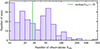 |
Fig. 1. Distribution of observations of 239 stars in the CARMENES jitter sample. The sample contains stars with at least ten RV measurements. The survey aims to obtain at least 50 observations per star. Stars with fewer than 50 measurements have not reached completion or were discontinued due to strong activity-related RV scatter (Ribas et al. 2023). |
The stellar parameters considered in this work are mainly taken from the CARMENES input catalog (Carmencita; Caballero et al. 2016). We used rotation periods from Shan et al. (2024). The stellar radii for the CARMENES survey sample were computed from effective temperatures and luminosities by Schweitzer et al. (2019). The average magnetic fields of CARMENES stars were determined by Reiners et al. (2022).
3. Method
We computed the RV jitter for the CARMENES sample. RV jitter refers to the excess noise in an RV time series (Baluev 2009). The uncertainty σi in each RV data point RVi is then given by the quadratic sum of its internal error σinternal, i and the excess noise σjitter, that is,  . When we model the probability density function of an RV measurement with a Gaussian distribution with a standard deviation σi and constant expected value μ, the log-likelihood function lnℒ of an RV time series is given by
![Mathematical equation: $$ \begin{aligned} \begin{aligned} \ln \mathcal{L}&= - \frac{1}{2} \sum \ln {\left(2 \pi \left[ \sigma _{\mathrm{internal} ,i}^2 + \sigma _{\mathrm{jitter} }^2\right]\right)} \\&\quad - \frac{1}{2} \sum {\frac{(\mathrm{RV} _i-\mu )^2}{\sigma _{\mathrm{internal} ,i}^2 + \sigma _{\mathrm{jitter} }^2}}\cdot \end{aligned} \end{aligned} $$](/articles/aa/full_html/2024/12/aa50836-24/aa50836-24-eq2.gif) (1)
(1)
We computed σjitter (and the time-series mean μ) by maximizing the log-likelihood function. To maximize the log-likelihood function in Eq. (1), we used the open-source script mlrms5. In Eq. (1), we made the intrinsic assumption of normally distributed data. Although signals such as sinusoids are non-Gaussian, their variance is captured by the jitter defined in Eq. (1). The jitter variance σjitter2 can be negative when the internal RV uncertainties are overestimated. For a negative jitter variance, the jitter values become imaginary. For formal reasons, we computed this imaginary jitter, but did not analyze them. To estimate the uncertainties of the derived jitter values, we applied the nonparametric bootstrapping method (Efron 1979). Therein, we drew 1000 samples with a replacement from each RV time series and computed the jitter in each sample. The standard deviation of the sample values represents our uncertainty estimate.
As an example, we show the CARMENES RV time series of EV Lac in Fig. 2. The internal uncertainties cannot explain the scatter of the data points. We call this scatter the external uncertainty σexternal and computed it as weighted RMS with weights  . For EV Lac, the RV jitter is close to the external uncertainty. EV Lac is a known active star, so that the high RV jitter value for EV Lac can be attributed to stellar activity (e.g. Jeffers et al. 2022), although the precise origin of the underlying signal is not relevant for the computation of the jitter.
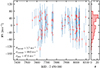 |
Fig. 2. Radial velocity time series of EV Lac (J22468+443). The radial velocities and internal uncertainties σinternal, i are displayed in red. The blue error bars indicate the quadratic sum of the internal uncertainties and the RV jitter |
A histogram of the resulting jitter values for slowly and fast-rotating stars as well as for the total sample is shown in Fig. 3. The distribution peaks at approximately 2 m s−1, and the median jitter lies at 3.1 m s−1. For 65 objects, we measure a jitter value lower than 2 m s−1. For 6 stars, we compute negative jitter variances indicating overestimated internal RV uncertainties. The star J19573−125 has the highest jitter value with 1120 ± 250 m s−1. The median RV jitter of only the slowly rotating stars (v sin i ≤ 2 km s−1) lies at 2.2 m s−1. The lower median jitter in slow rotators signifies a correlation between jitter and rotation. We study this in detail in Sect. 4.1.
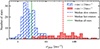 |
Fig. 3. Histogram showing the jitter of 233 CARMENES stars. Slowly rotating stars (v sin i ≤ 2 km s−1; striped blue bars) have a median jitter of 2.3 m s−1 (dashed blue line), and fast-rotating stars (v sin i > 2 km s−1; filled red bars) have a median jitter of 37 m s−1 (dashed red line). The median jitter for all stars is 3.1 m s−1 (solid green line). Six stars with negative jitter variances are not shown. |
4. Analysis and results
4.1. Jitter-rotation relation
On the disk of a rotating star, each surface element has an RV that depends on its projected distance to the rotation axis and on the stellar rotation period. The light emitted by each surface element is Doppler-shifted, and we observe a broadened line profile in the light that is integrated over the projected stellar disk. When a spot blocks a part of the stellar disk, the line becomes asymmetric, and an apparent velocity shift is induced. The variability of these shifts can lead to the RV variability that we recognize as jitter.
In Fig. 4, we show the relation between RV jitter and the equatorial rotation velocity veq. We computed veq from the stellar radius R⋆ and from the rotation period Prot as veq = 2π R⋆/Prot. The plot contains 129 CARMENES targets with stellar radii from Schweitzer et al. (2019) and rotation periods from Shan et al. (2024), who estimated the uncertainties of the rotation period using Eq. (4) of Shan et al. (2024). Stars with known planets were excluded (see Sect. 2). The jitter approaches a limit for slow rotators and increases for fast rotators, in agreement with a trend in veq. The observed increase in jitter with veq in the regime of fast rotation is expected for corotating star spots. A corotating star spot generates an RV signal with a semi-amplitude K ∝ veq.
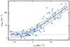 |
Fig. 4. Jitter-rotation relation for 129 CARMENES M dwarfs with known rotation periods. The RV jitter is fit as a function of the stellar rotation velocity veq. The solid line displays the best fit, and the shaded region indicates the prediction interval. The jitter floor and the linear trend (dashed lines) correspond to parameters α and β in Eq. (2). |
In addition, the amplitude of the spot signal is a function of the stellar inclination and limb darkening as well as of the spot parameter latitude, spot size, and contrast. The spot parameters are expected to vary with time, and hence, the spot amplitude is expected to vary with time. The spot configuration of individual stars is generally unknown and might vary significantly. Consequently, the dependences on spot parameters and inclination can be expected to smear out the jitter-rotation relation. All these effects may explain the variance around the general jitter trend in Fig. 4. The variance might also be a function of the sampling, namely the observation time-span and number of observations with respect to the rotation period. The jitter floor seen for slow rotation is caused by other sources of intrinsic stellar noise and instrumental effects. We discuss the jitter floor in detail in Sect. 5.1.
The relation between rotation and RV excess noise has traditionally been investigated using v sin i instead of veq (e.g. Saar & Donahue 1997). We used veq here because it can be computed for stars with very long rotation periods, allowing us to extend our analysis to stars that have only an upper limit on v sin i. Additionally, the uncertainties on v sin i are typically large compared to the formal uncertainties on veq. It might be expected that v sin i has a stronger correlation to σjitter and thus represents a better parameterization. For 53 stars in our dataset with both v sin i and veq detected (i.e., v sin i > 2 km s−1), the Pearson correlation coefficient between v sin i and σjitter is 0.62, and it is 0.64 between veq and σjitter. This shows that the correlation coefficients are similar for the fast-rotating stars.
The correlation between v sin i and veq is shown in Fig. 5. Following Shan et al. (2024), we mostly adopted v sin i values from Reiners et al. (2022) and assumed an uncertainty of 10% of their v sin i value, but a minimum uncertainty of 2 km s−1. An upper limit of 2 km s−1 was used for v sin i values below this limit because v sin i values below this limit cannot be obtained reliably (Reiners et al. 2018). One star, J06574+740, has inconsistent values of veq and v sin i; the values deviate by more than 2σ. The star shows an unusual beating pattern that might be related to binarity or to a complex spot pattern and stellar differential rotation (see discussion by Shan et al. 2024). Out of 159 stars with an upper limit on v sin i, 78 have values for veq that extend to ∼40 m s−1. Above v sin i = 2 km s−1, the data follow the expected trend for an isotropic distribution of the inclination angles.
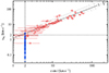 |
Fig. 5. Equatorial vs. projected rotation velocity. veq is derived from the stellar radius and rotation period, and v sin i originates from fitting the rotational line broadening. The blue dots display stars with an upper limit on v sin i, and red circles show stars with nominal values for v sin i. The dashed lines indicate 2 km s−1 in v sin i and veq. The linear |


In order to describe the jitter-rotation relation, we assumed that the jitter variance σjitter2 is the quadratic sum of a constant jitter floor, parameterized by α, and a jitter term linear in veq, parameterized by β, such that
 (2)
(2)
We fit the relation in logarithmic space using a maximum likelihood estimation (MLE) with emcee (Foreman-Mackey et al. 2013). The uncertainties of the jitter values were obtained by bootstrapping the RV data as described in Sect. 3. They do not necessarily represent the statistical uncertainties, but may rather result from the intrinsic variability of the stellar RV signal. We thus included the variance of the jitter as a nuisance parameter in our fit of the jitter-rotation relation (see Appendix A). The fit relation is displayed in Fig. 4, and the fit parameters are listed in Table 1. A corner plot of the fitting parameters is shown in Fig. F.12. The jitter floor lies at α=  m s−1, and the best-fit value for β is
  ⋅ 10−3. The jitter floor and the rotation term intersect (i.e., α = β ⋅ veq) at veq = 0.5 km s−1. The RMS around the jitter relation, which corresponds to the Δ in Eq. (2) and Fig. F.1, is 2.7 ± 0.2 dB2, corresponding to a factor of 1.9 of the upper and lower bounds of the prediction interval with respect to the expected jitter (Fig. F.1).
Best-fit parameters of the relations between jitter, equatorial rotation velocity, and average magnetic field strength.
The relation provides a good fit to the data in general. A deviation from the relation is visible for fast-rotating stars with veq higher than 3 km s−1. J04198+425, an M8.5-type star, is the most prominent outlier. It has a jitter value of 232 ± 43 m s−1 at an equatorial rotation velocity of veq = 5.70 ± 0.57 km s−1. The high-jitter bump also includes the well-known active stars YZ CMi and EV Lac. These high-jitter stars are likely young and posses strong average magnetic fields (Cortés-Contreras et al. 2024; Reiners et al. 2022). Additional information on the high-jitter stars (stars above the prediction interval displayed in Fig. 4) is provided in Appendix E2.
4.2. Average magnetic fields
In this section, we focus on the connection between average magnetic fields and RV jitter. The average magnetic fields of 292 CARMENES stars were measured by Reiners et al. (2022) by comparing polarized radiative transfer calculations with a selection of suitable observed spectral lines in the CARMENES coadded, high-S/N spectra. The lines were selected to represent a broad range of Landé g-factors, that is, sensitivities to the magnetic field, in order to differentiate from other broadening mechanisms. This allows for an accurate measurement of the magnetic field regardless of the rotational broadening. Upper limits were computed for stars with a weak magnetic field, which also have low rotation velocities (v sin i ≤ 2 km s−1).
A total of 178 stars of the 292 stars with a magnetic field measurement are part of our sample of stars with a sufficient number of observations and without indications of companions (see Sect. 2). For an additional 6 stars, the literature reports mean magnetic field measurements (Cristofari et al. 2023; Kochukhov 2021), but we did not include these to sustain the homogeneity of the sample. Figure 6 shows the RV jitter as a function of average magnetic field strength ⟨B⟩. For stars with an average magnetic field below 1 kG, the RV jitter stays below 10 m s−1. Between 1 to 3 kG, the RV jitter takes values from a few m s−1 to tens of m s−1. Above 3 kG, the RV jitter assumes high values up to several hundred m s−1. This regime of a high average magnetic field is also characterized by a weakened dependence of the magnetic field on rotation (see Fig. F.42).
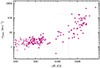 |
Fig. 6. Radial velocity jitter vs. mean magnetic field. The upper limits on the average magnetic field are indicated by triangles. |
We incorporated the average magnetic field into the jitter-rotation relation and tested different relations in order to minimize the scatter around the best-fitting model. A total of 89 stars have precise measurements of their average magnetic fields and equatorial rotation velocities. We allowed for additive and multiplicative terms of the average magnetic field and the equatorial rotation velocity to represent dependent and independent jitter generation. We also tested relations that only included one of the parameters, either the average magnetic field or the equatorial rotation velocity. The fit relations are listed in Table G.32. We applied the same fitting procedure as described in Sect. 4.1 and Appendix A.
To compare the models, we employed the Akaike information criterion (AIC; Akaike 1974) and the Bayesian information criterion (BIC; Schwarz 1978). According to Kass & Raftery (1995), an AIC or BIC difference smaller than 10 means that the comparison is indecisive, and an AIC or BIC difference smaller than 6 demonstrates only weak evidence in favor of the better-performing model. In our comparison, the three best-fitting relations produce a change in the BIC as well as AIC that is smaller than 6. This only suggests a weak preference for the best-fitting relation. The best-fitting relation with the lowest BIC and AIC values includes the average magnetic field strength. In this relation, the RV jitter is a function of the product of the equatorial rotation velocity veq and the average magnetic field strength ⟨B⟩, such that
 (3)
(3)
A single exponent for the product of ⟨B⟩ and veq instead of different exponents for both parameters is weakly preferred by our model comparison (see Table G.3). The model performs better than the jitter-rotation relation we fit in Sect. 4.1 (Eq. (2)) with a difference in BIC of 17.2. The best-fit relation (Eq. (3)) is shown in Fig. 7. The best-fit parameters are given in Table G.3, and the respective corner plot is shown in Fig. F.22). With α=  m s−1, the α-parameter takes a slightly higher value than α in the jitter-rotation relation without the average magnetic field (Eq. (2)). The slope parameter β is not directly comparable between Eqs. (2) and (3) because the average magnetic field and the additional exponent γ are included. The high-jitter stars lie closer to the expectation of the relation than in Fig. 4. J04198+425, which deviates most in Fig. 4, is not included because no measurement of the average magnetic field is available.
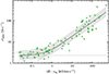 |
Fig. 7. Similar to Fig. 4, but showing the RV jitter as a function of the product of the average magnetic field strength and stellar rotation velocity for 89 CARMENES stars. Equation (3) is the functional form of the model. |
4.3. Magnetic field components
We previously showed in Sect. 4.1 that the observed RV jitter is related to the equatorial rotation velocity in fast rotators, and we showed that the RV jitter appears to be sensitive to the average magnetic field in Sect. 4.2. In this section, we investigate the impact of the distribution of the magnetic field filling factors.
The average magnetic field is the sum of the magnetic field components Bk, weighted by their filling factors fk, ⟨B⟩=∑kfkBk. The filling factors are derived from line profiles, which represent the sum of profiles emitted at different magnetic strengths and hence with different Zeeman broadening. Simplistically, the filling factors might be thought of as the relative area of the stellar disk that is penetrated by a magnetic field of a given magnetic field strength. The magnetic filling factors fk in the sum stated above are degenerate. In other words, stars with different magnetic filling factor distributions can have the same average magnetic field strength. We investigated the filling factor distributions of the stars in our sample based on the distributions fit by Reiners et al. (2022)6.
The filling factor distributions show different patterns, similar to the patterns described by Shulyak et al. (2019): Stars with small average magnetic field strengths have strong zero-field magnetic components. Stars with strong average magnetic field strengths display smooth distributions or concentrated distributions of the magnetic field components. In Fig. 8, we compare the filling factor distributions of EV Lac with those of J11201−104, which shows a broad distribution of magnetic field components ranging from 0–4 kG. Its zero component, that is, the contribution of regions with a magnetic field strength below 1 kG, has a filling factor of 0.25. In contrast, the filling factors in EV Lac follow a narrow distribution that peaks at 3kG and has a maximum filling factor of 0.43. The zero component is weak with a filling factor of 0.03. With veq = 4.55 ± 0.04 m s−1, J11201−104 has a similar rotation velocity as EV Lac. The average magnetic field strength is smaller in J11201−104 with 2170 ± 160 G.
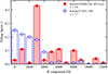 |
Fig. 8. Distribution of magnetic filling factors for EV Lac (solid red bars) and J11201−104 (dashed blue bars). The distribution index z indicates the concentration of the distribution of filling factors (see Eq. (4)). |
To characterize the shape of the filling factor distribution, we computed the significance of the largest peak other than ⟨B0⟩ = 0 G in relation to all other field strengths. That is, we quantified to which extent the star carries predominantly one particular field strength in contrast to a broad distribution of field strengths. For this purpose, we computed the mean and the standard deviation of the filling factors fk excluding the peak component. We defined a distribution index
 (4)
(4)
where fpeak = maxfk, k ≠ 0. The computed value serves as an indicator for the shape of the distribution: A high z value corresponds to a narrower distribution that is more strongly peaked, whereas a low z value corresponds to a more uniform distribution of the filling factors. When a negative value was obtained because a large zero component dominates the mean, we set the index to zero.
Figure 9 is a variation of our plot of the jitter-rotation relation, where the index of the filling factor distribution is now shown in the color-mapping. Stars with rotation velocities below 1 km s−1 have index values around zero, which is expected because their magnetic fields are weak. A series of stars between 4 to 10 km s−1 display high z-index values ≥5 as well as high jitter. These stars have similar narrow distributions with peaks between 2 to 4 kG. Their maximum filling factors lie between 0.35 to 0.55. J06574+740 is a possible extension of the series as it also shows a high z value, but a jitter value closer to the prediction by the jitter-rotation relation. The high-jitter stars with high z values are listed in Table 2. These stars are mid-M dwarfs, except for J08536−034, which is of spectral type M9V. All of these high-jitter stars are RV-loud by the definition of Tal-Or et al. (2018) since their v sin i values are higher than 2 km s−1 and their RV jitter values exceed 10 m s−1. The stars have Hα pseudo-equivalent widths pEW (Hα) ≤ −0.5 Å and can be considered as Hα-active following Jeffers et al. (2018).
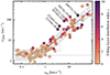 |
Fig. 9. As Fig. 4, but color-coded with the filling factor distributions index and only for stars with measured average magnetic field. The labels mark the series of high-jitter stars with concentrated magnetic field distributions. The empty circles display stars without measurements of the average magnetic field. |
Stellar parameters, RV jitter, and magnetic field properties of the series of high-jitter stars with concentrated magnetic field distributions.
The series of stars with excess jitter and a high z value also have a strong average magnetic field strength of 3.3–4.9 kG and are located at the upper end of the magnetic fields measured for CARMENES targets (Fig. 6). Additionally, four of the stars, J07446+035, J18131+260, J22468+443, and J23548+385, produce magnetic fields slightly more efficiently, as indicated by their Rossby numbers. Figure F.4 shows the average magnetic field as a function of the Rossby number. We include the relations fit by Shan et al. (2024, see their Fig. 9). J07446+035, J18131+260, J22468+443, and J23548+385 lie significantly above the relation at an Ro of around 0.3. J06574+740 and J08536−034 have lower Rossby numbers and lie close to the relation.
Figure 9 also displays stars with low z values and high jitter, and vice versa. Individual high-jitter stars are discussed in Appendix E2. The most prominent high-z stars with jitter below the prediction by the jitter-rotation relation are J05062+046 and J19511+464. Both stars occupy a similar region in the jitter-rotation plot around an equatorial rotation velocity of 30 km s−1 and a jitter value around 50 m s−1. The two stars are likely very young and are members of young stellar kinematic groups (Cortés-Contreras et al. 2024). Both stars have relatively few observations, 12 and 13.
Stars with high jitter and low z and vice versa might in general be explained by the following causes: (i) The variability of the RV signal of stars might not be completely sampled; many active stars only have about ten RV data points. Additionally, unaccounted-for trends might be present in these stars. (ii) The proposed index does not capture the full complexity of the magnetic field structure. (iii) The magnetic field measurements have large uncertainties, and the measurement reliability might decrease toward the regime of extreme rotation because the rotational line broadening increases.
5. Discussion
With our version of the jitter-rotation relation, we provide an extension of previous work toward slowly rotating stars on the basis of a large sample of well-characterized M dwarfs. In this section, we discuss the jitter floor, including possible contributions from instrumental effects, the implications of the jitter-rotation relation, and the connection of excess jitter to the magnetic field.
5.1. Jitter floor
Following previous analysis, we characterize RV jitter as excess noise, where we count any residual instrumental or stellar signal as noise. This has the advantage of a unified description of noise sources without major assumptions on the nature of the signal. With the jitter, we describe the regimes of slow stellar rotation, where the instrumental or stellar noise floor dominates, and fast rotation, where the rotation-related activity signal dominates.
In this framework, we exclude time series with fewer than ten data points and stars with known planets or trends. The minimum number of required data points was chosen arbitrarily. Consequently, the jitter can be over- or underestimated when only a part of the signal is sampled. This especially affects active stars, for which observations have often been deferred after their active nature was established. After completion, CARMENES will attain 50 observations for its survey stars (Ribas et al. 2023), which will allow for a more robust analysis in the future. For our analysis, we used data that were corrected for telluric absorption and NZPs. The telluric absorption correction (Nagel et al. 2023) has a large effect mainly on fast rotators, where the RV information content is relatively low because of rotational line broadening (e.g. Reiners et al. 2010). Hence, we reduced systematic telluric and instrumental effects to the best possible extent.
For stellar equatorial rotation velocities below ∼1 km s−1, we show that a jitter floor of approximately 2 m s−1 exists. The jitter floor might be caused by a baseline of stellar activity that is not related to rotation or instrumental instability. The signals of hidden companions also contribute to the observed jitter floor. Ribas et al. (2023) estimated that a fraction of  of M stars host planets when the planets in a mass bin of
  and periods of 1–1000 d are considered. Based on their assumptions (planet mass, orbital period distribution, and circular orbits), the median semi-amplitude of model planets in this parameter space lies at approximately 1.3 m s−1 (see Appendix C).
Instrumental instability might concern the accuracy of the wavelength solution, which is taken at the beginning of a night, or the accuracy of the drift measurements during the night (Schäfer et al. 2018). Nightly zero point shifts affect the accuracy of the wavelength solution and are identified by measuring the average Doppler shifts of RV-quiet stars in each night (Tal-Or et al. 2019; Ribas et al. 2023). Uncertainties on the NZPs are propagated to the corrected internal RV uncertainties used in this work. Therein, the NZP errors are typically ≲1 m s−1. Since NZP uncertainties are included in the internal RV uncertainties, nightly shifts should not contribute significantly to the jitter.
Ribas et al. (2023) reported a median reweighted RMS of 3.9 m s−1 for the NZP-corrected CARMENES RVs and a jitter contribution of 3.5 m s−1. Computing the jitter from spectra that were corrected for telluric absorption and excluding known planet hosts, we find a slightly lower median jitter of 3.1 m s−1.
In the following, we compare the jitter floor in CARMENES to the jitter floor in other RV surveys. Fischer et al. (2016) discussed the RV precision of the major Doppler search programs at the time. Their comparison was mostly based on the internal precision. The two largest programs in their comparison, executed with HARPS7 (Mayor et al. 2003) and HIRES8 (Vogt et al. 1994), provide an internal precision of 0.8 m s−1 and 1.5 m s−1, where the precision is scaled to a hypothetical observation with an S/N of 200 for a 3 km s−1 spectral bin at 550 nm. The median internal precision of all targets of the CARMENES survey lies at 1.6 m s−1, with a median S/N of 95. When we scale the precision to the hypothetical observation with S/N = 200, the CARMENES precision lies at 0.8 m s−1, which is similar to the precision of HARPS. Fischer et al. (2016) also provided RMS radial velocities of programs running on the various instruments. The California Planet Search appears to reach an RMS floor at 2–4 m s−1. The RMS in HARPS reaches 1–2 m s−1. Therefore, HARPS demonstrates the highest precision of the instruments compared by Fischer et al. (2016). However, a general comparison is only of limited use because internal as well as external precision also depends on the spectral type, among other parameters. Wright (2005) studied RV jitter in stars with F to M spectral types observed with HIRES. In inactive M dwarfs, they reported a jitter value of approximately 5 m s−1, which exceeds the median jitter in our sample by 2 m s−1. This might be related to the better instrumental stability of CARMENES, but it might also be due to differences in the samples. For the HARPS sample of M dwarfs, Bonfils et al. (2013) reported an internal uncertainty of down to 0.7 m s−1 and an external uncertainty between 1.5 to 2.0 m s−1 as a lower threshold for the brightest targets. The excess noise should consequently lie at 1.3–1.8 m s−1. Perger et al. (2017) reported an RV jitter of 2.3 m s−1 in their HARPS-N9 (Cosentino et al. 2012) survey of early-type M dwarfs. Tuomi et al. (2019) combined RV data of 426 nearby M dwarfs from HARPS, HIRES, UVES10 (Dekker et al. 2000), and PFS11 (Tamura et al. 2016). They obtained a median jitter of 2.3 m s−1. In a sample of 200 inactive mid- to late-type M dwarfs, Pass et al. (2023) reported internal uncertainties between 5 to 18 m s−1 for their most precise observations, and they measure a weighted standard deviation of 20 m s−1 and 21 m s−1 for the two instruments TRES12 (Szentgyorgyi & Furész 2007) and CHIRON13 (Tokovinin et al. 2013) that they employed. When we consider the internal uncertainty of 5 m s−1, the jitter floor in their survey lies at 9–11 m s−1, which suggests that their results are limited by instrumental noise.
The literature values as well as the jitter floor of  m s−1 determined in this work is overall compatible with a jitter floor of 1–3 m s−1 in M dwarfs. The question remains which contribution to the jitter floor dominates: instrumental, stellar jitter, or signals by unaccounted-for companions. We can attempt to estimate the contributions of instrumental noise, granulation jitter, and unaccounted companions. Bauer et al. (2020) investigated the instrumental stability of CARMENES in detail. They reported an instrumental jitter in CARMENES VIS of 1.2 m s−1. To approximate the granulation component of RV jitter, we used the scaling law by Luhn et al. (2020b, see their Eq. 9), which approximates the granulation-induced jitter as a function of stellar mass, luminosity, and effective temperature. For the stellar parameters of slowly rotating stars in our sample (v sin i ≤ 2 km s−1), we computed a granulation RV jitter up to 0.3 m s−1. We approximated the noise contribution caused by unaccounted-for companions with 0.9 m s−1 (see Appendix C). The combined jitter from the quadratic sum of these contributions is 1.5 m s−1, which agrees with the observed jitter floor established above.
The jitter floor does not represent a hard limit because planet searches have succeeded to detect planets with RV semi-amplitudes below 1 m s−1. Faria et al. (2022) claimed the detection of a planet with an RV semi-amplitude of 39 ± 7 cm s−1 around the slowly rotating mid-type M dwarf Proxima Centauri with ESPRESSO14 (Pepe et al. 2021). In addition to the two planets Proxima Centauri b and d, the RV signal was modeled using a Gaussian process with an RV amplitude of  m s−1 for the contribution of stellar RV signals. In the analysis, additional jitter terms of 0.07–0.40 m s−1 were retained. In this work, any stellar or other signal is modeled as jitter. When we consider the RV amplitude of the Gaussian process, the jitter floor of this work is thus consistent with the results of Faria et al. (2022).
5.2. Jitter-rotation relation
The linear part of our relation of RV jitter with the rotation velocity at fast rotation agrees in general with previous findings (Tal-Or et al. 2018; Saar et al. 1998). Saar et al. (1998) were the first to fit a power law in v sin i, finding a close-to-linear relation for F-, G-, and K-type stars. Subsequently, the RV jitter caused by the flux effect of cool star spots was studied many times also in numerical simulations (Saar & Donahue 1997; Hatzes 1999, 2002; Desort et al. 2007; Boisse et al. 2012; Dumusque et al. 2014; Herrero et al. 2016). These simulations demonstrated a linear (or almost linear) relation of a spot-induced RV amplitude with v sin i, which agrees with our observations in fast-rotating stars. They also found a linear relation with the spot filling factor (e.g. Saar & Donahue 1997). As stated by Boisse et al. (2012), a quantitative comparison between simulated and observed jitter relations is not a desirable approach because the models are constrained by simplifications and assumptions regarding the model parameters.
A linear scaling of the RV jitter with the projected rotation velocity is expected for the flux effect as long as the spot parameters stay constant as a function of rotation velocity. The observed trend (Fig. F.32) thus implies that spot parameters do not vary strongly with the rotation velocity in this regime. The activity-rotation relations predict increasing activity with increasing rotation velocity and saturation in fast-rotating stars. Most of the stars in the part that is dominated by activity and rotation in our plot in Fig. 4 belong to the stars in the saturated regime (see Fig. F.3).
Our fit of the linear part of the relation in Eq. (2) is mainly based on stars of type M4 and M5 because the CARMENES survey has a bias to early- and mid-type M dwarfs and mostly slow rotation in the early-type M dwarfs (Marfil et al. 2021). Furthermore, CARMENES contains only a few young stars (Cortés-Contreras et al. 2024). As a result of this bias, we cannot exclude deviations from the observed relation of jitter with rotation for early- and late-type M dwarfs and young M dwarfs. The jitter-rotation relation might change with spectral subtype and evolutionary state of a star.
The jitter-rotation relation allows us to estimate the expected RV jitter of M dwarfs given their rotation velocity. It might therefore be helpful in estimating detection limits of RV surveys as well as in preparing RV observations, such as the follow-up observations for mass determinations of transiting planets. Furthermore, an excess jitter compared to the jitter-rotation relation can be used as a quick indication of a planetary companion, in particular, for series with only a few measurements.
We show the predictive aspect of the relation for six stars from the CARMENES-TESS program (Table 3). CARMENES-TESS operated under the CARMENES GTO and Legacy surveys and followed-up planet candidates from the Transiting Exoplanet Survey Satellite mission (TESS; Ricker et al. 2015). The CARMENES-TESS stars were excluded from our jitter sample because they host planets. In Table 3, we predicted the RV jitter  based on the rotation period and stellar radius adopted in the respective CARMENES-TESS publication and using Eq. (2). The raw TAC RVs of TOI-442 jitter with
  m s−1, which significantly exceeds our prediction from stars without planets. TOI-1201 and TOI-1801 are close to the upper edge of the prediction interval. No quick conclusions about the presence of planets can be made for the remaining three stars. When the planetary signals are removed, the remaining jitter should also be consistent with the prediction. As a proxy for the remaining jitter
  , we used the jitter given in the CARMENES-TESS publications. Since the stellar activity is typically taken out mostly by Gaussian processes (GP; Rajpaul et al. 2015), we quadratically added the GP amplitude back. These jitters
  agree well with our predictions. Thus, our prediction can serve as a simple planet indicator that is even applicable for a few data points.
Comparison of predicted and observed jitter for six CARMENES-TESS stars.
5.3. Role of the magnetic field
The jitter-rotation relation describes the trend of RV jitter with rotation. Aiming to reduce the scatter in this relation, we included the average magnetic field strength in the relation. The improved relation is a function of the product of the average magnetic field with the equatorial rotation velocity.
The increased jitter floor in stars with strong magnetic fields indicates the suppression of convective shifts by the presence of magnetic fields. We observed a difference of 0.5 ± 0.4 m s−1 in the fitted jitter floor between the jitter-rotation relation (Eq. (2)) and the relation that additionally included the average magnetic field (Eq. (3)). To further investigate this difference in the jitter floor, we compared the mean jitter of stars with and without strong magnetic fields in the slowest rotators of our sample (veq < 0.5 km s−1). The mean jitter of stars with weak magnetic fields (only upper limits on the average magnetic field strength) is lower by 0.5 ± 0.3 m s−1. This difference in the jitter floor could be caused by the suppression of convective shifts by strong magnetic fields. Variability in the magnetic field results in a variable suppression of convective shifts and could thus produce RV jitter regardless of rotational modulation and the flux effect.
The average magnetic field saturates in fast-rotating stars Reiners et al. (2022). A saturation of the average magnetic field with the equatorial rotation velocity can also be seen (Fig. F.3). The saturation in fast-rotating stars might correspond to saturation in the expression of the surface features, such as spots. In this case, we would expect that RV jitter increases with rotation velocity at a slower rate for stars in the saturated regime. A saturation would affect stars with a rotation velocity upward of approximately 5 km s−1. No saturation is clearly visible in our plot of the RV jitter against the equatorial rotation velocity (Fig. 4). However, the improved fit including the average magnetic field (Eq. (3)) compared to the rotation-only fit (Eq. (2)) may result from a slight saturation of the RV jitter in fast-rotating stars.
A correlation between the magnetic field strength and RV jitter in M dwarfs was previously investigated by Moutou et al. (2017). Moutou et al. (2017) proposed an activity merit function based on the total chromospheric emission, the absolute longitudinal magnetic field, v sin i, and the average magnetic field. From the weights of the parameters of their merit function, the authors concluded that most of the jitter is explained by the longitudinal magnetic field and chromospheric emission. In contrast, we observe that jitter is primarily a function of rotation (Sects. 4.1 and 4.2). Their sample mostly consisted of slow rotators, many only with upper limits on v sin i, such that the effect of rotation likely is less prevalent in their sample.
A series of stars that showed excess jitter compared to the jitter-rotation relation also showed similar distributions of their magnetic field components, with a single dominating magnetic field component at 2–4 kG. The filling factors of the dominant component lie between 0.35 to 0.55. Shulyak et al. (2019) previously noted the similarity of the magnetic filling factor distributions between YZ CMi, EV Lac, and J23548+385. It now appears that this type of distribution extends to the entire group of stars with excess jitter, and the excess jitter in these stars appears to be related to the shape of their magnetic filling factor distributions. We characterize the shape of magnetic filling factor distribution with the index z defined in Eq. (4). The stars of the excess-jitter group have an index value between z= 7 to 9, which is significantly above the mean for all filling factor distributions of our sample at 1.6.
The high z values in the excess-jitter stars is indicative of a correlation between the magnetic filling factor distribution and the RV jitter. The distribution does not reveal the spatial distribution of the magnetic field on the stellar surface. It is therefore unclear whether the dominant component is associated with specific features on the stellar surface, that is, spots or faculae, or is distributed rather homogeneously over the stellar surface.
Active stars exhibit a variety of magnetic filling factor distributions, and it has been suggested that different distributions are related to different dynamo states (Reiners et al. 2022; Shulyak et al. 2019). Although it is unclear why the stars show different distributions, the distributions appear to affect the RV jitter. RV jitter arises from corotating spatial inhomogeneities, that is, it requires a difference in the magnetic field or temperature. Therefore, magnetic field or temperature differences must exist in the stars with excess jitter, even though their magnetic field components are concentrated in the range of 2–4 kG. These excess-jitter stars also have low filling factors for magnetic field components below B = 2 kG. This implies that the magnetic field or temperature difference that causes the RV jitter is between wide spread regions with strong magnetic fields, and not between small regions of spots and faculae against the backdrop of a quiet stellar surface.
Presumably, the RV signal of a spot on a star with an overall active surface changes compared to a spot on a star that is predominantly inactive because the stellar surface brightness strongly changes with magnetic field strength (Norris et al. 2023) and the spectrum is altered by the Zeeman effect. Simulations should consider the concentration of magnetic field components, such as observed in the excess-jitter stars, in order to better understand the influence of the magnetic field on the stellar RV signal. Another pathway is the detailed study of individual magnetically sensitive lines such as the strong KI lines in the near-infrared (Fuhrmeister et al. 2022; Terrien et al. 2022).
We suspect that the increased RV jitter in the stars with concentrated magnetic field components is related to the line shape of magnetically sensitive lines. Each line in the spectrum carries RV information depending on the line shape, with sharp lines carrying more RV information than broad lines (Bouchy et al. 2001). As a result of the Zeeman effect, magnetically sensitive lines split in the presence of magnetic fields, where the splitting is proportional to the magnetic field strength. The resulting Zeeman components of the line are therefore sharper for a narrow distribution of the magnetic field components and broader for a wide distribution of the magnetic field components. Consequently, the Zeeman components of a line carry more RV information in the case of a narrow distribution of the magnetic field components. Hence, we expect the magnetically sensitive lines to have greater RV information in stars with concentrated magnetic field components than in stars with a broad distribution of the magnetic field components. Greater RV information in the magnetically sensitive lines means that these lines contribute more to the total RV. We therefore expect magnetic field variability to cause larger RV jitter in stars with concentrated magnetic field components.
6. Summary
We measured the jitter in the RV time series of M dwarfs from the CARMENES survey. The CARMENES VIS RV jitter correlates with the rotation velocity, which we computed from stellar rotation period and stellar radius. We fit a relation of the RV jitter as a function of rotation velocity,
 (5)
(5)
The relation can be used to predict jitter, where the prediction has to be multiplied (divided) by 1.9 to obtain upper (lower) bounds. In stars rotating slower than 1 km s−1, the RV jitter is independent of stellar rotation. Thus, the remaining jitter must result from residual instrumental noise, hidden companions, and granulation. We conclude that the reduction of rotationally modulated variability is not sufficient to reach below the jitter floor of ∼2 m s−1 in our survey.
The effect of the average magnetic field on the RV jitter was considered as an extension of the jitter-rotation relation. A relation of the RV jitter as function of the product of the average magnetic field and rotation velocity is preferred to the jitter-rotation relation without a magnetic field. The best-fitting relation with a magnetic field is given by
 (6)
(6)
A series of stars with excess jitter shares a distinctive distribution of the magnetic filling factors, which is characterized by magnetic filling factors that are concentrated around 2–4 kG. We conclude that the concentration of magnetic filling factors affects the Zeeman-split line profiles and leads to the observed excess jitter. The identification of distinctive magnetic field components in stars with excess RV jitter suggests that activity-induced RV signals are associated with specific distributions of the magnetic field components.
Data availability
Full Table D.1 is available at the CDS via anonymous ftp to cdsarc.cds.unistra.fr or via https://cdsarc.cds.unistra.fr/viz-bin/cat/J/A+A/692/A138. Appendices E to G are available in electronic form on Zenodo via https://doi.org/10.5281/zenodo.13889774.
Calar Alto high-Resolution search for M dwarfs with Exoearths with Near-infrared and optical Échelle Spectrographs.
Available on Zenodo via https://doi.org/10.5281/zenodo.13889774
The component distributions of all stars with average magnetic field measurements are available in their supplement (http://carmenes.cab.inta-csic.es/gto/jsp/reinersetal2022.jsp).
High Accuracy Radial velocity Planet Searcher.
High Resolution Echelle Spectrometer.
High Accuracy Radial velocity Planet Searcher for the Northern hemisphere.
Ultraviolet and Visual Echelle Spectrograph.
Subaru Prime Focus Spectrograph.
Tillinghast Reflector Echelle Spectrograph.
CTIO HIgh ResolutiON spectrograph.
Echelle SPectrograph for Rocky Exoplanets and Stable Spectroscopic Observations.
Acknowledgments
This publication was based on observations collected under the CARMENES Legacy+ project. CARMENES is an instrument at the Centro Astronómico Hispano en Andalucía (CAHA) at Calar Alto (Almería, Spain), operated jointly by the Junta de Andalucía and the Instituto de Astrofísica de Andalucía (CSIC). The authors wish to express their sincere thanks to all members of the Calar Alto staff for their expert support of the instrument and telescope operation. CARMENES was funded by the Max-Planck-Gesellschaft (MPG), the Consejo Superior de Investigaciones Científicas (CSIC), the Ministerio de Economía y Competitividad (MINECO) and the European Regional Development Fund (ERDF) through projects FICTS-2011-02, ICTS-2017-07-CAHA-4, and CAHA16-CE-3978, and the members of the CARMENES Consortium (Max-Planck-Institut für Astronomie, Instituto de Astrofísica de Andalucía, Landessternwarte Königstuhl, Institut de Ciències de l’Espai, Institut für Astrophysik Göttingen, Universidad Complutense de Madrid, Thüringer Landessternwarte Tautenburg, Instituto de Astrofísica de Canarias, Hamburger Sternwarte, Centro de Astrobiología and Centro Astronómico Hispano-Alemán), with additional contributions by the MINECO, the Deutsche Forschungsgemeinschaft (DFG) through the Major Research Instrumentation Programme and Research Unit FOR2544 “Blue Planets around Red Stars”, the Klaus Tschira Stiftung, the states of Baden-Württemberg and Niedersachsen, and by the Junta de Andalucía. We acknowledge financial support from the Agencia Estatal de Investigación (AEI/10.13039/501100011033) of the Ministerio de Ciencia e Innovación and the ERDF “A way of making Europe” through projects PID2022-137241NB-C4[1:4], PID2021-125627OB-C31, and the Centre of Excellence “Severo Ochoa” and “María de Maeztu” awards to the Instituto de Astrofísica de Canarias (CEX2019-000920-S), Instituto de Astrofísica de Andalucía (CEX2021-001131-S) and Institut de Ciències de l’Espai (CEX2020-001058-M). This work was also funded by the Generalitat de Catalunya/CERCA programme, the DFG priority program SPP 1992 “Exploring the Diversity of Extrasolar Planets” through grants JE 701/5-1 and RE 1664/20-1, and the Israel Science Foundation through grant 1404/22. We thank the anonymous reviewer for helpful comments.
References
- Akaike, H. 1974, IEEE Trans. Autom. Control, 19, 716 [Google Scholar]
- Al Moulla, K., Dumusque, X., Figueira, P., et al. 2023, A&A, 669, A39 [NASA ADS] [CrossRef] [EDP Sciences] [Google Scholar]
- Alonso-Floriano, F. J., Morales, J. C., Caballero, J. A., et al. 2015, A&A, 577, A128 [NASA ADS] [CrossRef] [EDP Sciences] [Google Scholar]
- Baluev, R. V. 2009, MNRAS, 393, 969 [Google Scholar]
- Baroch, D., Morales, J. C., Ribas, I., et al. 2020, A&A, 641, A69 [EDP Sciences] [Google Scholar]
- Bauer, F. F., Zechmeister, M., Kaminski, A., et al. 2020, A&A, 640, A50 [NASA ADS] [CrossRef] [EDP Sciences] [Google Scholar]
- Beeck, B., Cameron, R. H., Reiners, A., & Schüssler, M. 2013, A&A, 558, A49 [NASA ADS] [CrossRef] [EDP Sciences] [Google Scholar]
- Boisse, I., Bonfils, X., & Santos, N. C. 2012, A&A, 545, A109 [NASA ADS] [CrossRef] [EDP Sciences] [Google Scholar]
- Bonfils, X., Delfosse, X., Udry, S., et al. 2013, A&A, 549, A109 [NASA ADS] [CrossRef] [EDP Sciences] [Google Scholar]
- Bouchy, F., Pepe, F., & Queloz, D. 2001, A&A, 374, 733 [NASA ADS] [CrossRef] [EDP Sciences] [Google Scholar]
- Brandenburg, A., & Subramanian, K. 2005, Phys. Rep., 417, 1 [NASA ADS] [CrossRef] [Google Scholar]
- Caballero, J. A., Cortés-Contreras, M., Alonso-Floriano, F. J., et al. 2016, 19th Cambridge Workshop on Cool Stars, Stellar Systems, and the Sun (CS19), 148 [Google Scholar]
- Cortés-Contreras, M., Caballero, J. A., Montes, D., et al. 2024, A&A, in press, https://doi.org/10.1051/0004-6361/202451585 [Google Scholar]
- Cosentino, R., Lovis, C., Pepe, F., et al. 2012, Proc. SPIE, 8446, 84461V [Google Scholar]
- Crass, J., Gaudi, B. S., Leifer, S., et al. 2021, ArXiv e-prints [arXiv:2107.14291] [Google Scholar]
- Cristofari, P. I., Donati, J. F., Folsom, C. P., et al. 2023, MNRAS, 522, 1342 [NASA ADS] [CrossRef] [Google Scholar]
- Dekker, H., D’Odorico, S., Kaufer, A., Delabre, B., & Kotzlowski, H. 2000, Proc. SPIE, 4008, 534 [Google Scholar]
- Desort, M., Lagrange, A. M., Galland, F., Udry, S., & Mayor, M. 2007, A&A, 473, 983 [CrossRef] [EDP Sciences] [Google Scholar]
- Díez Alonso, E., Caballero, J. A., Montes, D., et al. 2019, A&A, 621, A126 [NASA ADS] [CrossRef] [EDP Sciences] [Google Scholar]
- Donati, J. F., Cristofari, P. I., Finociety, B., et al. 2023, MNRAS, 525, 455 [NASA ADS] [CrossRef] [Google Scholar]
- Dravins, D., & Ludwig, H.-G. 2023, A&A, 679, A3 [NASA ADS] [CrossRef] [EDP Sciences] [Google Scholar]
- Dreizler, S., Crossfield, I. J. M., Kossakowski, D., et al. 2020, A&A, 644, A127 [EDP Sciences] [Google Scholar]
- Dumusque, X., Boisse, I., & Santos, N. C. 2014, ApJ, 796, 132 [NASA ADS] [CrossRef] [Google Scholar]
- Efron, B. 1979, Ann. Stat., 7, 1 [Google Scholar]
- Ellwarth, M., Schäfer, S., Reiners, A., & Zechmeister, M. 2023, A&A, 673, A19 [NASA ADS] [CrossRef] [EDP Sciences] [Google Scholar]
- Faria, J. P., Suárez Mascareño, A., Figueira, P., et al. 2022, A&A, 658, A115 [NASA ADS] [CrossRef] [EDP Sciences] [Google Scholar]
- Fischer, D. A., Anglada-Escude, G., Arriagada, P., et al. 2016, PASP, 128, 066001 [Google Scholar]
- Foreman-Mackey, D., Hogg, D. W., Lang, D., & Goodman, J. 2013, PASP, 125, 306 [Google Scholar]
- Fuhrmeister, B., Czesla, S., Nagel, E., et al. 2022, A&A, 657, A125 [NASA ADS] [CrossRef] [EDP Sciences] [Google Scholar]
- Goffo, E., Chaturvedi, P., Murgas, F., et al. 2024, A&A, 685, A147 [NASA ADS] [CrossRef] [EDP Sciences] [Google Scholar]
- Hatzes, A. P. 1999, ASP Conf. Ser., 185, 259 [NASA ADS] [Google Scholar]
- Hatzes, A. P. 2002, Astron. Nachr., 323, 392 [NASA ADS] [CrossRef] [Google Scholar]
- Haywood, R. D., Milbourne, T. W., Saar, S. H., et al. 2022, ApJ, 935, 6 [NASA ADS] [CrossRef] [Google Scholar]
- Herrero, E., Ribas, I., Jordi, C., et al. 2016, A&A, 586, A131 [NASA ADS] [CrossRef] [EDP Sciences] [Google Scholar]
- Hudson, H. S. 1988, ARA&A, 26, 473 [NASA ADS] [CrossRef] [Google Scholar]
- Isaacson, H., & Fischer, D. 2010, ApJ, 725, 875 [Google Scholar]
- Jeffers, S. V., Schöfer, P., Lamert, A., et al. 2018, A&A, 614, A76 [NASA ADS] [CrossRef] [EDP Sciences] [Google Scholar]
- Jeffers, S. V., Barnes, J. R., Schöfer, P., et al. 2022, A&A, 663, A27 [NASA ADS] [CrossRef] [EDP Sciences] [Google Scholar]
- Jenkins, J. S., Ramsey, L. W., Jones, H. R. A., et al. 2009, ApJ, 704, 975 [Google Scholar]
- Kass, R. E., & Raftery, A. E. 1995, J. Am. Stat. Assoc., 90, 773 [Google Scholar]
- Kochukhov, O. 2021, A&ARv, 29, 1 [Google Scholar]
- Kossakowski, D., Kemmer, J., Bluhm, P., et al. 2021, A&A, 656, A124 [NASA ADS] [CrossRef] [EDP Sciences] [Google Scholar]
- Kossakowski, D., Kürster, M., Henning, T., et al. 2022, A&A, 666, A143 [NASA ADS] [CrossRef] [EDP Sciences] [Google Scholar]
- Kürster, M., Endl, M., Rouesnel, F., et al. 2003, A&A, 403, 1077 [NASA ADS] [CrossRef] [EDP Sciences] [Google Scholar]
- Liebing, F., Jeffers, S. V., Reiners, A., & Zechmeister, M. 2021, A&A, 654, A168 [NASA ADS] [CrossRef] [EDP Sciences] [Google Scholar]
- Lienhard, F., Mortier, A., Cegla, H. M., et al. 2023, MNRAS, 522, 5862 [NASA ADS] [CrossRef] [Google Scholar]
- Ludwig, H. G., Allard, F., & Hauschildt, P. H. 2002, A&A, 395, 99 [NASA ADS] [CrossRef] [EDP Sciences] [Google Scholar]
- Luhn, J. K., Wright, J. T., & Isaacson, H. 2020a, AJ, 159, 236 [NASA ADS] [CrossRef] [Google Scholar]
- Luhn, J. K., Wright, J. T., Howard, A. W., & Isaacson, H. 2020b, AJ, 159, 235 [Google Scholar]
- Luque, R., Pallé, E., Kossakowski, D., et al. 2019, A&A, 628, A39 [NASA ADS] [CrossRef] [EDP Sciences] [Google Scholar]
- Luque, R., Fulton, B. J., Kunimoto, M., et al. 2022, A&A, 664, A199 [NASA ADS] [CrossRef] [EDP Sciences] [Google Scholar]
- Mallorquín, M., Goffo, E., Pallé, E., et al. 2023, A&A, 680, A76 [NASA ADS] [CrossRef] [EDP Sciences] [Google Scholar]
- Marfil, E., Tabernero, H. M., Montes, D., et al. 2021, A&A, 656, A162 [NASA ADS] [CrossRef] [EDP Sciences] [Google Scholar]
- Mayor, M., Pepe, F., Queloz, D., et al. 2003, The Messenger, 114, 20 [NASA ADS] [Google Scholar]
- Moutou, C., Hébrard, E. M., Morin, J., et al. 2017, MNRAS, 472, 4563 [NASA ADS] [CrossRef] [Google Scholar]
- Nagel, E., Czesla, S., Kaminski, A., et al. 2023, A&A, 680, A73 [NASA ADS] [CrossRef] [EDP Sciences] [Google Scholar]
- Norris, C. M., Unruh, Y. C., Witzke, V., et al. 2023, MNRAS, 524, 1139 [NASA ADS] [CrossRef] [Google Scholar]
- Pass, E. K., Winters, J. G., Charbonneau, D., et al. 2023, AJ, 166, 11 [NASA ADS] [CrossRef] [Google Scholar]
- Pepe, F., Cristiani, S., Rebolo, R., et al. 2021, A&A, 645, A96 [NASA ADS] [CrossRef] [EDP Sciences] [Google Scholar]
- Perger, M., García-Piquer, A., Ribas, I., et al. 2017, A&A, 598, A26 [NASA ADS] [CrossRef] [EDP Sciences] [Google Scholar]
- Quirrenbach, A., Amado, P. J., Caballero, J. A., et al. 2016, Proc. SPIE, 9908, 990812 [Google Scholar]
- Rajpaul, V., Aigrain, S., Osborne, M. A., Reece, S., & Roberts, S. 2015, MNRAS, 452, 2269 [Google Scholar]
- Reiners, A. 2012, Liv. Rev. Sol. Phys., 9, 1 [Google Scholar]
- Reiners, A., Basri, G., & Browning, M. 2009, ApJ, 692, 538 [NASA ADS] [CrossRef] [Google Scholar]
- Reiners, A., Bean, J. L., Huber, K. F., et al. 2010, ApJ, 710, 432 [Google Scholar]
- Reiners, A., Joshi, N., & Goldman, B. 2012, AJ, 143, 93 [Google Scholar]
- Reiners, A., Zechmeister, M., Caballero, J. A., et al. 2018, A&A, 612, A49 [NASA ADS] [CrossRef] [EDP Sciences] [Google Scholar]
- Reiners, A., Shulyak, D., Käpylä, P. J., et al. 2022, A&A, 662, A41 [NASA ADS] [CrossRef] [EDP Sciences] [Google Scholar]
- Ribas, I., Reiners, A., Zechmeister, M., et al. 2023, A&A, 670, A139 [NASA ADS] [CrossRef] [EDP Sciences] [Google Scholar]
- Ricker, G. R., Winn, J. N., Vanderspek, R., et al. 2015, JATIS, 1, 014003 [Google Scholar]
- Saar, S. H., & Donahue, R. A. 1997, ApJ, 485, 319 [Google Scholar]
- Saar, S. H., Butler, R. P., & Marcy, G. W. 1998, ApJ, 498, L153 [NASA ADS] [CrossRef] [Google Scholar]
- Schäfer, S., Guenther, E. W., Reiners, A., et al. 2018, Proc. SPIE, 10702, 1070276 [Google Scholar]
- Schwarz, G. 1978, Ann. Stat., 6, 461 [Google Scholar]
- Schweitzer, A., Passegger, V. M., Cifuentes, C., et al. 2019, A&A, 625, A68 [NASA ADS] [CrossRef] [EDP Sciences] [Google Scholar]
- Seifahrt, A., Bean, J. L., Kasper, D., et al. 2022, Proc. SPIE, 12184, 121841G [NASA ADS] [Google Scholar]
- Shan, Y., Revilla, D., Skrzypinski, S. L., et al. 2024, A&A, 684, A9 [NASA ADS] [CrossRef] [EDP Sciences] [Google Scholar]
- Shulyak, D., Reiners, A., Nagel, E., et al. 2019, A&A, 626, A86 [NASA ADS] [CrossRef] [EDP Sciences] [Google Scholar]
- Skumanich, A. 1972, ApJ, 171, 565 [Google Scholar]
- Suárez Mascareño, A., Rebolo, R., González Hernández, J. I., & Esposito, M. 2017, MNRAS, 468, 4772 [Google Scholar]
- Szentgyorgyi, A. H., & Furész, G. 2007, Rev. Mex. Astron. Astrofis., 28, 129 [NASA ADS] [Google Scholar]
- Tal-Or, L., Zechmeister, M., Reiners, A., et al. 2018, A&A, 614, A122 [NASA ADS] [CrossRef] [EDP Sciences] [Google Scholar]
- Tal-Or, L., Trifonov, T., Zucker, S., Mazeh, T., & Zechmeister, M. 2019, MNRAS, 484, L8 [Google Scholar]
- Tamura, N., Takato, N., Shimono, A., et al. 2016, Proc. SPIE, 9908, 99081M [NASA ADS] [CrossRef] [Google Scholar]
- Terrien, R. C., Keen, A., Oda, K., et al. 2022, ApJ, 927, L11 [NASA ADS] [CrossRef] [Google Scholar]
- Tokovinin, A., Fischer, D. A., Bonati, M., et al. 2013, PASP, 125, 1336 [NASA ADS] [CrossRef] [Google Scholar]
- Tuomi, M., Jones, H. R. A., Butler, R. P., et al. 2019, ArXiv e-prints [arXiv:1906.04644] [Google Scholar]
- Vogt, S. S., Allen, S. L., Bigelow, B. C., et al. 1994, Proc. SPIE, 2198, 362 [Google Scholar]
- Wright, J. T. 2005, PASP, 117, 657 [Google Scholar]
- Zechmeister, M., Reiners, A., Amado, P. J., et al. 2018, A&A, 609, A12 [NASA ADS] [CrossRef] [EDP Sciences] [Google Scholar]
- Zechmeister, M., Dreizler, S., Ribas, I., et al. 2019, A&A, 627, A49 [NASA ADS] [EDP Sciences] [Google Scholar]
Appendix A: Log-likelihood function jitter-rotation relation
We fit the jitter-rotation relation in logarithmic space. In logarithmic space, Eq. (2) takes the shape of
 (A.1)
(A.1)
In order to perform an unweighted fit, we assume the variance Δ2 is constant in all data points. We treat Δ as a nuisance parameter, hence its value is obtained from the fit itself. Performing the fit in logarithmic space effectively weights down data points with large values, since residuals in logarithmic space correspond to relative rather than absolute deviations in the original space.
Best-fit values are obtained from MLE. The log-likelihood lnℒ including the nuisance parameter Δ2 for the variance is given by
![Mathematical equation: $$ \begin{aligned} \ln \mathcal{L} = -\frac{1}{2} \sum _i \left[ \frac{(\log {\sigma }_{\mathrm{jitter} ,i} - \log {\sigma }_{\mathrm{jitter} }(\alpha ,\beta ,v_{\mathrm{eq} ,i}))^2}{\Delta ^2} + \ln \left( 2\pi \,\Delta ^2 \right) \right]. \end{aligned} $$](/articles/aa/full_html/2024/12/aa50836-24/aa50836-24-eq45.gif) (A.2)
(A.2)
Appendix B: Expected value of the sine of the inclination
The inclination i is in [0, π/2]. The probability density function (pdf) of cos i is uniform for isotropic distributed stellar spin axes
 (B.1)
(B.1)
Then, the pdf g(i) of the inclination i can be computed as
 (B.2)
(B.2)
The expected value of sin i is then given by
 (B.3)
(B.3)
The expected value of  is then given by
 (B.4)
(B.4)
Appendix C: Hidden companions
The RV signals of hidden companions can contribute to the observed RV jitter. Thus, we compare the RV semi-amplitude of planets from a model distribution to the observed RV jitter. We study the signals of potential low-mass planets, as they lie at the sensitivity threshold of the CARMENES survey.
Ribas et al. (2023) find that a fraction of  of M stars host planets when considering the planets in a mass bin of
  and periods of 1 to 1000 d. The occurrence rate is computed applying the assumption of a log-uniform distribution of orbital periods. They fit a power-law dependence of the number of planets Npl as function of their minimum mass Mplsin i, where Npl ∝ (Mplsin i)α. For the coefficient α, they find a value of −1.05 ± 0.01.
To compute an expected RV semi-amplitude, we randomly draw from the log-uniform distribution of orbital periods, and from a power-law distribution of minimum mass fitted by Ribas et al. (2023). We also randomly draw a stellar mass from our sample of slowly rotating stars with veq < 1 km s−1. From period, minimum mass, and stellar mass, we then compute the RV semi-amplitude. We repeat the experiment for 106 iterations using a Markov chain Monte Carlo (MCMC) approach. The resulting distribution is shown in Fig. C.1. We overplot a histogram of jitter in slow rotating stars with veq < 1 km s−1, where the jitter is not dominated by the modulation of the stellar rotation. The amplitudes of the modeled planet population are not sufficient to explain the observed jitter. However, we also see that the RV semi-amplitudes of approximately a fourth of the model planets have semi-amplitudes within 1 to 2 m s−1. The median semi-amplitude lies at 1.3 m s−1, corresponding to a jitter of 0.9 m s−1 (under the assumption of circular orbits and evenly sampled RV time series). Thus, hidden planets likely contribute to the observed jitter floor.
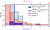 |
Fig. C.1. RV semi-amplitude distribution of model planet distribution. The observed jitter in CARMENES of stars with and without known planets (blue and light blue bars) is compared to the RV semi-amplitudes of the model planet population (red hatched bars). The median RV semi-amplitude (red line) lies at 1.3 m s−1, and the median RV jitter of stars with and without planets (blue line) is 2.1 m s−1. |
Appendix D: CARMENES VIS jitter sample
Stellar properties and jitter of the 239 targets in the CARMENES VIS jitter sample.a
All Tables
Best-fit parameters of the relations between jitter, equatorial rotation velocity, and average magnetic field strength.
Stellar parameters, RV jitter, and magnetic field properties of the series of high-jitter stars with concentrated magnetic field distributions.
Stellar properties and jitter of the 239 targets in the CARMENES VIS jitter sample.a
All Figures
|
Fig. 1. Distribution of observations of 239 stars in the CARMENES jitter sample. The sample contains stars with at least ten RV measurements. The survey aims to obtain at least 50 observations per star. Stars with fewer than 50 measurements have not reached completion or were discontinued due to strong activity-related RV scatter (Ribas et al. 2023). |
| In the text | |
|
Fig. 2. Radial velocity time series of EV Lac (J22468+443). The radial velocities and internal uncertainties σinternal, i are displayed in red. The blue error bars indicate the quadratic sum of the internal uncertainties and the RV jitter |
| In the text | |
|
Fig. 3. Histogram showing the jitter of 233 CARMENES stars. Slowly rotating stars (v sin i ≤ 2 km s−1; striped blue bars) have a median jitter of 2.3 m s−1 (dashed blue line), and fast-rotating stars (v sin i > 2 km s−1; filled red bars) have a median jitter of 37 m s−1 (dashed red line). The median jitter for all stars is 3.1 m s−1 (solid green line). Six stars with negative jitter variances are not shown. |
| In the text | |
|
Fig. 4. Jitter-rotation relation for 129 CARMENES M dwarfs with known rotation periods. The RV jitter is fit as a function of the stellar rotation velocity veq. The solid line displays the best fit, and the shaded region indicates the prediction interval. The jitter floor and the linear trend (dashed lines) correspond to parameters α and β in Eq. (2). |
| In the text | |
|
Fig. 5. Equatorial vs. projected rotation velocity. veq is derived from the stellar radius and rotation period, and v sin i originates from fitting the rotational line broadening. The blue dots display stars with an upper limit on v sin i, and red circles show stars with nominal values for v sin i. The dashed lines indicate 2 km s−1 in v sin i and veq. The linear |
| In the text | |
|
Fig. 6. Radial velocity jitter vs. mean magnetic field. The upper limits on the average magnetic field are indicated by triangles. |
| In the text | |
|
Fig. 7. Similar to Fig. 4, but showing the RV jitter as a function of the product of the average magnetic field strength and stellar rotation velocity for 89 CARMENES stars. Equation (3) is the functional form of the model. |
| In the text | |
|
Fig. 8. Distribution of magnetic filling factors for EV Lac (solid red bars) and J11201−104 (dashed blue bars). The distribution index z indicates the concentration of the distribution of filling factors (see Eq. (4)). |
| In the text | |
|
Fig. 9. As Fig. 4, but color-coded with the filling factor distributions index and only for stars with measured average magnetic field. The labels mark the series of high-jitter stars with concentrated magnetic field distributions. The empty circles display stars without measurements of the average magnetic field. |
| In the text | |
|
Fig. C.1. RV semi-amplitude distribution of model planet distribution. The observed jitter in CARMENES of stars with and without known planets (blue and light blue bars) is compared to the RV semi-amplitudes of the model planet population (red hatched bars). The median RV semi-amplitude (red line) lies at 1.3 m s−1, and the median RV jitter of stars with and without planets (blue line) is 2.1 m s−1. |
| In the text | |
Current usage metrics show cumulative count of Article Views (full-text article views including HTML views, PDF and ePub downloads, according to the available data) and Abstracts Views on Vision4Press platform.
Data correspond to usage on the plateform after 2015. The current usage metrics is available 48-96 hours after online publication and is updated daily on week days.
Initial download of the metrics may take a while.