| Issue |
A&A
Volume 691, November 2024
|
|
|---|---|---|
| Article Number | A294 | |
| Number of page(s) | 14 | |
| Section | Extragalactic astronomy | |
| DOI | https://doi.org/10.1051/0004-6361/202451766 | |
| Published online | 20 November 2024 | |
Multi-epoch jet outbursts in Abell 496: Synchrotron ageing and buoyant X-ray cavities draped by warm gas filaments
1
Dipartimento di Fisica e Astronomia, Università di Bologna, via Gobetti 93/2, I-40129 Bologna, Italy
2
Istituto Nazionale di Astrofisica – Osservatorio di Astrofisica e Scienza dello Spazio (OAS), via Gobetti 101, I-40129 Bologna, Italy
3
Naval Research Laboratory, 4555 Overlook Avenue SW, Code 7213, Washington, DC 20375, USA
4
NASA/Goddard Space Flight Center, Greenbelt, MD 20771, USA
5
Istituto Nazionale di Astrofisica - Istituto di Radioastronomia (IRA), via Gobetti 101, I-40129 Bologna, Italy
6
Center for Astrophysics | Harvard & Smithsonian, 60 Garden Street, Cambridge, MA 02138, USA
⋆ Corresponding author; This email address is being protected from spambots. You need JavaScript enabled to view it.
Received:
2
August
2024
Accepted:
20
September
2024
Abstract
Aims. The galaxy cluster Abell 496 has been extensively studied in the past for the clear sloshing motion of its hot intracluster medium (ICM) on large scales, but the interplay between the central radio galaxy and the surrounding cluster atmosphere is mostly unexplored. We present a dedicated radio, X-ray, and optical study of Abell 496 with the aim being to investigate this connection.
Methods. We use deep radio images obtained with the Giant Metrewave Radio Telescope (GMRT) at 150, 330, and 617 MHz, the Very Large Array (VLA) at 1.4 and 4.8 GHz, and the VLA Low Band Ionosphere and Transient Experiment (VLITE) at 340 MHz, with angular resolutions ranging from 0.″5 to 25″. Additionally, we use archival Chandra and Very Large Telescope (VLT) MUSE observations.
Results. The radio images reveal three distinct periods of jet activity: an ongoing episode on subkiloparsec scales with an inverted radio spectrum; an older episode that produced lobes on scales of ∼20 kpc, which now have a steep spectral index (α = 2.0 ± 0.1); and an even older episode that produced lobes on scales of ∼50 − 100 kpc with an ultrasteep spectrum (α = 2.7 ± 0.2). Archival Chandra X-ray observations show that the older and oldest episodes excavated two generations of cavities in the hot gas of the cluster. The outermost X-ray cavity has a clear mushroom-head shape, likely caused by its buoyant rise in the cluster’s potential. Cooling of the hot gas is ongoing in the innermost 20 kpc, where warm, Hα-bright filaments are visible in VLT-MUSE data. The Hα-filaments are stretched toward the mushroom-head cavity, which may have stimulated ICM cooling in its wake. We conclude by discussing our nondetection of a radio mini-halo in this vigorously sloshing but low-mass galaxy cluster.
Key words: galaxies: clusters: general / galaxies: clusters: intracluster medium / galaxies: clusters: individual: Abell 496 / radio continuum: general / X-rays: galaxies: clusters
© The Authors 2024
 Open Access article, published by EDP Sciences, under the terms of the Creative Commons Attribution License (https://creativecommons.org/licenses/by/4.0), which permits unrestricted use, distribution, and reproduction in any medium, provided the original work is properly cited.
This article is published in open access under the Subscribe to Open model. This email address is being protected from spambots. You need JavaScript enabled to view it. to support open access publication.
1. Introduction
Radio galaxies represent clear manifestations of jet launching from active galactic nuclei (AGN). The lobes of these objects, extending from either side of the central engine, provide a wealth of informative about how AGN interact with and influence their surrounding environment (e.g., Hardcastle & Croston 2020; Bourne & Yang 2023). This is especially relevant for radio galaxies at the centers of galaxy clusters with cool cores. Cool-core clusters, which are characterized by a central region of lower gas temperature compared to the surrounding intracluster medium (ICM), present a unique environment for radio-lobe evolution. The expanding radio lobes often push aside the ICM, creating depressions in the X-ray-emitting gas (e.g., McNamara & Nulsen 2007, 2012).
The active phase of a super massive black hole (SMBH) is not continuous. Periods of intense jet activity can be followed by quiescent phases, leaving behind the remnants of past outbursts (e.g., Hardcastle & Croston 2020). After detaching from the jets, the radio lobes age and further expand in the ICM. Radio-filled cavities have a lower density than the surrounding ICM, leading to a buoyant rise of these structures towards the cool core outskirts (blackat distances from the center of ∼100 kpc; e.g., Churazov et al. 2001). As these bubbles rise, they can entrain the surrounding ICM in their wake, stimulating cooling instabilities in the hot gas and condensation to cooler gas phases (e.g., Voit & Donahue 2015). The evolution of bubbles at later times is more uncertain: theoretical models predict that efficient shear instabilities and mixing should cause bubbles to lose their integrity and eventually become disrupted, unless viscosity or magnetic field stabilize them against instabilities (e.g., Reynolds et al. 2005; Sijacki & Springel 2006; Brighenti et al. 2015).
Addressing these issues with observations requires a fortunate combination of sensitivity, spatial resolution, and frequency coverage, because (a) the oldest radio lobes are inherently fainter due to energy losses in the relativistic electrons, the magnitude of which can only be determined by employing multifrequency radio observations; (b) the corresponding X-ray cavities reside in the outskirts of, or beyond, the cool core, and thus their contrast in X-ray images is relatively low; and (c) resolving the features caused by instabilities requires high spatial resolution. So far, the stability of buoyant bubbles has been studied only for the radio lobes and bubbles in Virgo and Perseus (e.g., Churazov et al. 2001; Kaiser et al. 2005; Roediger et al. 2013), which are respectively the closest and most X-ray bright clusters.
In this work, we address the above topics in Abell 496 (hereafter A496), a nearby cool core galaxy cluster (z = 0.0329, cooling radius ∼70 kpc) extensively studied in the X-ray band for the clear bulk motions (sloshing) of its ICM on large scales (Dupke & White 2003; Tanaka et al. 2006; Dupke et al. 2007; Roediger et al. 2012; Ghizzardi et al. 2014). One of the most interesting features of this cluster is the irregular and boxy shape of its cold fronts (surface-brightness edges caused by the bulk motions of the gas), which suggests the presence of Kelvin-Helmholtz instabilities in the ICM at the interface of the edges (Roediger et al. 2012; Ghizzardi et al. 2014). However, the properties of the radio galaxy at the center of this cluster have so far been neglected. The available information is mainly from the sample studies of Hogan et al. (2015a,b), who report the presence of radio emission with an ultrasteep radio spectrum at sub-GHz frequencies (indicative of particles aging) and radio emission with a flat spectrum above 1 GHz (indicative of renewed SMBH activity). In the present paper, we leverage multifrequency radio observations of A496, as well as X-ray and Hα data, to study the central radio source of this cluster and its interaction with the hot gas.
We summarize the general properties of A496 in Table 1. We adopt a ΛCDM cosmology with H0 = 70 km s−1 Mpc−1, Ωm = 0.3, and ΩΛ = 0.7. At the redshift of A496 (z = 0.0329), 1″ corresponds to 0.656 kpc. The radio spectral index α is defined according to Sν ∝ ν−α, where Sν is the flux density at the frequency ν.
Properties of the galaxy cluster A496.
2. Radio observations
We analyzed pointed observations of A496 retrieved from the Giant Metrewave Radio Telescope (GMRT) and Very Large Array (VLA) archives, covering a frequency interval from 330 MHz to 4.9 GHz and with an angular resolution ranging from  to ∼20″. Our analysis also includes data at 340 MHz from the VLA Low Band Ionosphere and Transient Experiment (VLITE, Clarke et al. 2016), a commensal system that operates on the VLA. Finally, we reanalyzed GMRT data at 150 MHz from three fields of the TIFR GMRT Sky Survey (TGSS1) that contain A496 within their field of view. Table 2 summarizes the details of all radio observations processed in this paper.
Summary of the radio observations.
2.1. GMRT data
We retrieved observations at 150 MHz, 330 MHz, and 617 MHz from the GMRT archive. All data were collected in spectral-line mode using the hardware back-end. A total observing bandwidth of 16 MHz was used at 150 MHz and 330 MHz. Two 16 MHz bands (upper and lower side bands, USB/LSB) were instead used at 617 MHz, for a total bandwidth of 32 MHz. Below, we provide a description of the data reduction at each of these frequencies.
2.1.1. Observations at 150 MHz and 330 MHz
We reduced the data using the National Radio Astronomy Observatory (NRAO) Astronomical Image Processing System (AIPS2, Greisen 2003). We used RFLAG to excise visibilities affected by radio frequency interference (RFI), followed by manual flagging to remove residual bad data. Gain and bandpass calibrations were applied using the primary calibrators (Table 2). Their flux density at 150 MHz and 330 MHz was set based on the Scaife & Heald (2012) scale. Phase calibrators observed several times during the observation were used to calibrate the data in phase. A number of phase self-calibration cycles were applied to the target visibilities, followed by a final self-calibration step in amplitude. Non-coplanar effects were taken into account using wide-field imaging at all frequencies, decomposing the primary beam area (half-power beamwidth ∼186′ at 150 MHz and ∼81′ at 330 MHz) into smaller facets. Additional facets were placed on bright outlier sources out to a radius of 10° from the center. Small clean masks were placed by hand around all sources in the imaged field. Finally, to improve the dynamic range of our images, we used PEELR to “peel” (see e.g., Noordam 2004) a bright radio source (PKS0431–133), located ∼10′ from the A496 center, whose strong side-lobe pattern affects the cluster region at all frequencies. At 150 MHz, the three TGSS fields were calibrated and imaged separately. The final images were restored with a common beam of 24″ × 18″, corrected for the GMRT primary-beam attenuation, and finally combined together in the image plane.
The primary beam correction was done with PBCOR using the appropriate primary-beam shape parameters at each frequency3. Table 3 summarizes the restoring beams and root mean square (rms) noise levels (1σ) of our final GMRT images, which were obtained by setting the Briggs robustness weighting (Briggs 1995) to zero during the clean in IMAGR. Residual amplitude errors are estimated to be within 15% at 150 MHz and 10% at 327 MHz (Chandra et al. 2004).
Summary of the radio images.
2.1.2. Observations at 617 MHz
We used the Source Peeling and Atmospheric Modeling (SPAM; Intema et al. 2009) pipeline4 to process the archival GMRT observation at 617 MHz (Table 2). We adopted a standard calibration scheme that consists of bandpass and complex gain calibration and direction-independent self-calibration, followed by direction-dependent self-calibration. The flux density scale was set using 3C 48 and Scaife & Heald (2012). The USB and LSB datasets were processed individually. The final self-calibrated data sets were then converted into measurement sets using the Common Astronomy Software Applications (CASA5, version 5.1 CASA Team 2022) and finally imaged together using the joint and multi-scale deconvolution options in WSClean (Offringa et al. 2014; Offringa & Smirnov 2017) with a Briggs robust parameters of zero. Correction for the GMRT primary-beam response was applied using the AIPS task PBCOR. Our final image at 617 MHz has a beam of 6″ × 5″ and a noise of 0.35 mJy/beam (Table 3). The systematic amplitude uncertainty is estimated to be within 10% (Chandra et al. 2004).
2.2. VLA data
We reprocessed seven archival VLA multi-configuration and multifrequency observations of A496 (Table 2) using AIPS and following a standard procedure of gain and bandpass calibration. The flux density scale was set using SETJY and the Perley & Butler (2017) coefficients for the primary calibrator sources listed in Table 2. The data were calibrated in phase using phase-calibration sources observed during the observations. Several loops of imaging and phase-only self-calibration were applied to reduce the effects of residual phase and amplitude errors in the data. During the imaging process, we used small clean masks around the sources. All images were made using a Briggs robust parameter of zero. The two B-configuration images at 1.4 GHz were first restored with a common 4″ circular beam and then combined together into a final image with a noise of 1σ = 100 μJy beam−1. Correction for the VLA primary beam attenuation was applied to all images. Table 3 summarizes the restoring beams and rms values. Residual amplitude errors are within 5% at all frequencies.
2.3. VLITE data
VLITE is a commensal, low-frequency system on the VLA Clarke et al. (2016). It operates in parallel with nearly all regular observing programs above 1 GHz and provides real-time correlation of the signal from a subset of VLA antennas (up to 18) using the low-band receiver system (Clarke et al. 2011) and dedicated DiFX-based software (Deller et al. 2007). The VLITE system processes 64 MHz of bandwidth centered on 352 MHz; however, due to strong RFI in the upper portion of the band, the usable frequency range is limited to an RFI-free band of ∼40 MHz centered on 338 MHz.
On 2021 February 15, VLITE recorded data with 17 antennas during a VLA observation at the primary frequency of 1.5 GHz of A496 (project 20B-138; Table 2), when the VLA was in A configuration. The VLITE data were processed using a dedicated calibration and imaging pipeline, which is based on a combination of Obit (Cotton 2008) and AIPS data reduction packages. The pipeline uses standard automated tasks for the removal of RFI, followed by delay, complex gain, and bandpass calibration (for details see Polisensky et al. 2016). The flux density scale is set using Perley & Butler (2017) and residual amplitude errors are estimated to be within 15% (Clarke et al. 2016). The calibrated data are imaged using wide-frequency imaging algorithms in Obit (task MFImage), by covering the full primary beam with facets and placing outlier facets on bright sources out to a radius of 20°. Clean masks are placed on the sources during the imaging process to reduce the effects of CLEAN bias. The pipeline runs two imaging and phase self-calibration cycles before a final image is created.
For A496, the pipeline produced an image with a beam of 7″ × 4″ and 1.3 mJy/beam rms. To increase the image sensitivity, we re-imaged the pipeline-calibrated data with WSClean using a higher number of cleaning iterations than in the automated pipeline and a cleaning mask generated from the pipeline image. Our final VLITE image has a resolution of 7″ × 4″ (for ROBUST = 0) and an improved sensitivity of 1σ = 0.66 mJy/beam (Table 3).
3. Complementary data
3.1. Chandra X-ray observations
A496 was observed by Chandra in 2000 for 18.9 ks (ObsID 931, ACIS-S, faint mode), in 2001 for 10 ks (ObsID 3361, ACIS-S, very faint mode), and in 2004 for 75 ks (ObsID 4976, ACIS-S, very faint mode). We reprocessed the event files in CIAO 4.14 (Fruscione et al. 2006) using the Chandra Calibration Database (CALDB) 4.9.7 and standard procedures of calibrations (e.g., Wang et al. 2016), obtaining a cleaned exposure time of 65.3 ks (63% of total time). To model the detector and sky background, we used the blank-sky data sets from the CALDB appropriate for the date of observation. The blank-sky data set was reprojected onto the sky using the aspect information and normalized using the ratio of the observed to blank-sky count rates in the 9.5–12 keV band. We obtained background-subtracted and exposure-corrected images of the cluster in the 0.5–4 keV and 0.5–7 keV energy bands. Spectral analysis was performed in the 0.5–7 keV band using Xspec-v12.12.1, selecting the table of solar abundances of Asplund et al. (2009). An absorption component (tbabs) was always included to account for Galactic absorption, with the column density fixed at NH = 4.3 × 1020 cm−2 (HI4PI Collaboration 2016), and the redshift fixed at z = 0.0329.
3.2. VLT-MUSE observations
To complement our radio and X-ray analysis, we employ optical observations of A496 performed with the Very Large Telescope using the MUSE integral-field spectrograph (here we consider the observation 094.B-0592). The MUSE data were reduced using the MUSE pipeline 2.8.5 (Weilbacher et al. 2014). The average seeing of the data is 0.8″. We fit the spectrum of each spaxel using the PLATEFIT code (Tremonti et al. 2004; Brinchmann et al. 2004; see also e.g., Olivares et al. 2019 for a similar application) to derive a map of intensity and kinematics of the Hα emission line, which is sensitive to the extended warm gas nebula surrounding the central dominant (cD) galaxy.
4. Radio images of A496
In this section, we present our radio images of the central source in A496 at multiple angular resolutions and frequencies, which allow us to identify different components of emission on different spatial scales.
4.1. Compact component and inner lobes
Figure 1 presents our high-resolution (∼2″) image at 1.5 GHz (blue colour and contours) overlaid on a Hubble Space Telescope (HST) Wide Field and Planetary Camera 2 (WFPC2) image of the cluster central galaxy (Observation ID U62G1902R). The radio emission (hereafter referred to as inner source) consists of a bright central and compact component, coincident with the galaxy optical peak, and a pair of asymmetric, diffuse, and very faint radio lobes. The lobes extend ∼10 kpc to the northeast (NE) and ∼5 kpc to the southwest (SW). No defined, kiloparsec(kpc)-scale jets are visible within their diffuse emission.
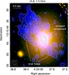 |
Fig. 1. VLA A–configuration image at 1.5 GHz (blue and contours) of the central radio source in A496, overlaid on the optical HST WFPC2 image of the central galaxy (orange). The restoring beam of the radio image is 2″ × 1″, at a position angle (PA) of 17° (boxed white ellipse in the bottom left corner) and the noise level is 1σ = 50 μJy beam−1. Contours are spaced by a factor of 2 starting from +3σ. |
In Fig. 2 we show the VLITE 340 MHz, GMRT 617 MHz, VLA-B 1.4 GHz, and VLA-C 4.7 GHz images of the inner source. The central component and inner lobes are detected on a similar scale of ∼25 kpc in panels (a), (b), and (c). At 4.7 GHz (d), the emission is clearly dominated by the compact component and only part of the NE inner lobe is detected.
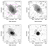 |
Fig. 2. Radio images of the inner source in A496. (a): VLITE 340 MHz image. The beam is 7″ × 4″, in PA −2° and noise is 1σ = 0.66 mJy/beam. (b): GMRT 617 MHz image. The beam is 6″ × 5″, in PA −54° and 1σ = 0.47 mJy/beam. (c): VLA–B configuration combined image at 1.4 GHz. The image has been restored with a 5″ circular beam. The noise is 1σ = 0.1 mJy/beam. (d): VLA–C configuration image at 4.7 GHz. The image has been restored with a 4″ circular beam. The noise is 1σ = 0.03 mJy/beam. In all panels, contours are spaced by a factor of 2 starting from +3σ. Contours at −3σ mJy/beam are shown as dashed lines. The boxed ellipse or circle shows the beam size. The white cross marks the optical peak (Fig. 1). In panel (a), the magenta box is as in Fig. 3. |
4.2. Outer radio lobes
Figure 3 presents our low-frequency GMRT images at 150 MHz6 and 330 MHz. The images are shown on the same spatial scale. As a reference, the magenta box marks the area occupied by the inner lobes and compact component (Fig. 2a). A pair of large-scale radio lobes are detected in both images. The lobe axis is close to that of the inner lobes in Fig. 2; however both lobes seem to slightly bend at large distance from the center. The total extent of the source at these low frequencies is ∼100 kpc.
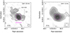 |
Fig. 3. Radio images of the outer radio lobes in A496. (a): GMRT image at 330 MHz (grayscale and contours). The image has been restored with a 12″ circular beam and the noise is 1σ = 0.5 mJy/beam. (b): GMRT combined image at 150 MHz (grayscale and contours). The restoring beam is 24″ × 18″, in PA 0° and 1σ = 10 mJy/beam. In both panels, contours are spaced by a factor of 2 starting from +3σ. No contours at −3σ are present in the portion of the image shown. The boxed ellipse or circle shows the beam size. The magenta box marks the area occupied by the inner double source (see Fig. 2a). The white cross marks the optical peak (Fig. 1). |
5. Radio flux densities and spectral analysis
In this section we measure the total flux densities and radio spectrum of the central source in A496 and of its different components using the images listed in Table 3. We complement our measurements with flux densities from the literature and from radio surveys, including the VLA Low-frequency Sky Survey Redux (VLSSr, Lane et al. 2014) at 74 MHz, the Galactic and Extragalactic All-Sky MWA survey (GLEAM, Hurley-Walker et al. 2017) at 76–227 MHz, the Rapid ASKAP Continuum Survey (RACS, McConnell et al. 2020; Hale et al. 2021) at 888 MHz, and the VLA Sky Survey (VLASS, Lacy et al. 2020) at 3 GHz. For a proper comparison, we have rescaled all the flux density values used in this paper to a common flux density scale. We adopted the Perley & Butler (2017) scale, which is valid between 50 MHz and 50 GHz, and used appropriate scaling factors based on Perley & Butler (2017). Differences between the original and Perley & Butler (2017) scales are estimated to be within 5%.
5.1. Total emission
We measured the total radio emission at the cluster center by integrating our images within a circular region of  in radius (∼60 kpc) centered on the radio peak (RAJ200 = 04h33m38s, DecJ2002 = −13° 15′43″). For the images at 4.8 GHz and 4.9 GHz in B and A configurations, where only the central compact component is detected, the total flux density was measured via a Gaussian fit on the images. Our measurements are summarized in Table 4. Errors were computed including the image rms and flux calibration uncertainty. The table includes complementary flux densities from the 74 MHz VLSSr and 888 MHz RACS images (measured within the same
  region), catalog values from the GLEAM survey, and higher-frequency measurements reported in the literature from the Australia Telescope Compact Array (Hogan et al. 2015a), Effelsberg (Andernach et al. 1988), CARMA, and GISMO (Hogan et al. 2015b). The 3 GHz measurements are from the VLASS quick-look images from Epochs 1.2, 2.1, and 3.1, where only the compact source is detected. The corresponding flux densities were calculated using a Gaussian fit to the source on the quick-look images and corrected for low-flux-density biases of 15% (VLASS 1.2) and 8% (VLASS 2.1 and 3.1), which affect faint sources, as reported in the NRAO Quick-Look Image web page7. A total uncertainty of 10% was assumed for the VLASS values. As mentioned above, all flux density values are on the same Perley & Butler (2017) scale, with the exception of the measurements at 90 GHz (CARMA) and 150 GHz (GISMO).
Total flux density of the radio galaxy in A496.
The spectrum of the whole radio emission is shown in Fig. 4 (left) with data points from our images highlighted in violet. A similar spectrum, but with fewer data points, was presented by Hogan et al. (2015b). The overall shape of the spectrum is complex and clearly inconsistent with a simple power-law behavior. The spectral index is very steep (α ∼ 1.5) at frequencies of lower than 1.4 GHz, it flattens to α ∼ 0.4 between 1.4 GHz and 10.7 GHz, and then steepens again to α ∼ 0.9 between 10.7 GHz and 150 GHz. The flattening and curving of the spectrum above 1.4 GHz suggests the presence of an active component that dominates the emission at high frequencies. The steepening below 1.4 GHz suggests, instead, the presence of an aged, extended component that emerges predominantly at low frequencies. To further investigate these spectral features, we examined the spectrum of the individual components in the system.
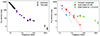 |
Fig. 4. Spectra of the radio source at the center of A496. Left: integrated radio spectrum of the total radio emission at the center of A496. Our flux density measurements are shown as purple filled squares. Catalog and literature values from Table 4 are shown in black. Right: radio spectra of the individual components. The blue dashed line shows the spectral slope of the outer lobes. The dashed pink line and shaded area represent the best fit and associated uncertainty with a CI-off model to the spectrum of the inner lobes. The VLBA 5 GHz flux density from Ubertosi et al. (2024) is plotted with a gold circle. |
5.2. Central compact component
We measured the flux density of the central compact component (Figs. 1 and 2) by fitting the source with a Gaussian model. At 340 MHz and 617 MHz, we used images made using only baselines longer than 20 kλ (sensitive to structures smaller than a few kpc). Our flux densities are summarized in Table 5, which also includes the 3 GHz flux densities from the VLASS 1.2, 2.1, and 3.1 quick-look images (see Sect. 5.1) and higher-frequency measurements from the literature. The spectrum of the central component in the 340 MHz–150 GHz interval is shown in Fig. 4 (right) as green data points. The central source has a steep, high-frequency spectrum (α ∼ 0.7 above 5 GHz) and a flat, possibly inverted spectrum below 5 GHz. This is similar to the spectral behavior of GHz-peaked spectrum (GPS) radio sources (e.g., Stanghellini et al. 1997; O’Dea & Saikia 2021), which are interpreted as an early stage in the evolution of a radio galaxy. The similarity suggests that the central compact source represents the onset of a new phase of activity of the central AGN.
Flux densities of the compact component.
This is consistent with the detection of a radio core in Very Long Baseline Array (VLBA) archival data at 5 GHz (project BE056), as recently shown by Ubertosi et al. (2024). In the VLBA image that we show in Fig. 5, twin jets are seen emanating from the core in the NE-SW direction (position angle of about 140°), and the source has a largest linear size of 15 mas (10 parsecs). The core has a flux density at 5 GHz of 44.3 ± 4.3 mJy, whereas the jets have a combined flux density of 12.6 ± 1.3 mJy. The total of about 57 ± 6 mJy represents ∼100% of the flux density detected at kpc scales from the VLA at around 5 GHz (Fig. 2d, Fig. 4 right, and Table 5). This supports the scenario of the central compact source being a recently renewed radio galaxy.
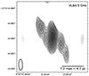 |
Fig. 5. VLBA image at 5 GHz of the compact component in A496 at a resolution of 3.5 × 1.2 mas and with noise of σ = 60 μJy/beam. Contours start at 5σ and increase by a factor of 2. |
5.3. Radio lobes
The flux densities of the inner lobes are summarized in Table 6, along with the associated uncertainties and the observed spectral index measured between the lowest and highest frequencies available. At frequencies of ≥340 MHz, the lobe flux density was estimated by subtracting the contribution of the compact component (Table 5) from the total emission in the area shown in Fig. 2a. At 150 MHz and 330 MHz, the angular resolution of our images does not allow us to separate the compact source from the surrounding extended emission. Therefore, in Table 6, we report the total flux density (inner lobes + compact source) measured within the magenta box in Fig. 3a. Based on its flat spectrum at GHz frequencies (Fig. 4, right), we estimate that the contribution of the compact component is at most ∼10% at 330 MHz, and less than ∼4% at 150 MHz.
Flux densities and spectral index of the lobes.
The outer lobes are clearly detected only in our images at 150 MHz and 330 MHz. We measured their flux density at these frequencies as the difference between the total emission (Table 4) and the inner emission (inner lobes and compact source; Table 6), obtaining 830 ± 115 mJy at 150 MHz and 99 ± 10 mJy at 330 MHz (Table 6).
In Fig. 4 (right), the spectra of the inner and outer lobes are shown in red and blue, respectively. The spectrum of the inner lobes has a steep slope of α = 1.5 ± 0.1 between 150 MHz and 617 MHz and it further steepens to α = 2.3 ± 0.1 at higher frequencies. The outer lobes have an even steeper spectrum with α = 2.7 ± 0.2 in the 150–330 MHz interval. These steep indices suggest that both pairs of lobes are old and possibly associated with former cycle(s) of activity of the central galaxy.
Moreover, the diffuse morphology of the inner lobes and the presence of a renewed outburst on parsec scales indicate that the inner lobes are no longer powered by active jets. Thus, we fitted their spectrum using SYNCHROFIT8 (Quici et al. 2022) with a CI-off model, which assumes an initial phase of electron injection at a constant rate (continuous injection; CI) by the nuclear source, followed by a dying phase during which the radio emission fades (e.g., Murgia et al. 2011). We assume a uniform magnetic field within the source and an isotropic distribution of the pitch angle of the radiating electrons. Prior to fitting, we set the magnetic field to the equipartition value of Beq = 22 μG estimated from the 1.4 GHz map9 of Fig. 2 and using the equations reported in Govoni & Feretti (2004). The resulting best fit for the spectrum of the inner lobes (pink line in Fig. 4) gives a total age of ttot = 26 ± 4 Myr, with an active phase of ton = 20 ± 3 Myr in duration and a passive phase of toff = 6 ± 1 Myr.
Given the limited availability of only two points in the spectrum of the outer lobes, we are unable to derive their synchrotron ages. In any case, their ultrasteep spectrum between 150 and 330 MHz (with α = 2.7 ± 0.2) strongly suggests that they are older than the inner lobes. We can derive an approximate radiative age using the following equation (e.g., Eilek 2014):
![Mathematical equation: $$ \begin{aligned} t_{\text{rad}}[\text{ Myr}] = \frac{1590\sqrt{B}}{\left(B^{2} + B_{\rm CMB}^{2}\right)\sqrt{1+z}}\sqrt{\frac{(\alpha -\Gamma )\text{ ln}\left(\frac{\nu _{2}}{\nu _{1}}\right)}{\nu _{2} - \nu _{1}}} ,\end{aligned} $$](/articles/aa/full_html/2024/11/aa51766-24/aa51766-24-eq4.gif) (1)
(1)
where B and BCMB = 3.25(1 + z)2 are the source and the cosmic microwave background magnetic fields, respectively (μG), and Γ is the injection index (assumed equal to 0.7; e.g., Eilek 2014). For B ∼ 1 − 20 μG, we find trad ∼ 50 − 300 Myr. We caution that this estimate is an approximation, and we can at most argue that the radiative age of the outer lobes is of the order of ∼108 yr.
5.4. Spectral index image
A spectral index image in the low-frequency interval 150–330 MHz is shown in Fig. 6, along with the associated error map. The image was obtained by comparing a pair of primary-beam-corrected images produced with the same cell size, uv range (0.06 − 12.2 kλ), and restoring beam of 24″ × 18″. Only pixels with a signal-to-noise ratio of 3 or larger were considered.
 |
Fig. 6. Color-scale image of the spectral index distribution between 150 MHz and 330 MHz (a) and the associated error map (b), computed from primary-beam-corrected images with the same uv range and beam of 24″ × 18″. The spectral index was calculated in each pixel where the surface brightness is above the 3σ level in both images. Overlaid are the 330 MHz contours, spaced by a factor of 2 from 3σ = 3 mJy/beam. The white box marks the region occupied by the inner double source (Fig. 2a). The white cross marks the optical peak (Fig. 1). |
The image confirms that the spectral index in the outer lobes is very steep (α ∼ 2.5 − 3, with a typical spectral index uncertainty of ∼0.2). The central region that encloses the inner lobes (white box) is characterized by a peak with α ∼ 0.7, surrounded by steeper-spectrum emission with values of up to ∼2.
6. Connection between radio, X–ray, and Hα emission
A496 is known for its four striking concentric cold fronts: three of them located within the central r ∼ 70 kpc region (Dupke & White 2003; Dupke et al. 2007) and the most distant one at ∼160 kpc from the center (Ghizzardi et al. 2014; see also Tanaka et al. 2006). Here, we focus on the details of the X-ray emission within the cooling region (r ∼ 70 kpc) and its relation to the extended radio features associated with the cD galaxy.
In Fig. 7 we show the X-ray emission detected by Chandra at increasing distance from the center. The core structure inside the innermost cold front, shown in panel (a), is characterized by a bright, curved feature –possibly the tip of the sloshing spiral seen at larger scale– and a number of small surface brightness depressions distributed around the position of the cD galaxy (marked by the green cross). At larger scale (b), the most prominent feature is the spiral structure traced by the cold fronts (marked by white lines). A region of X-ray-emission deficit is visible to the NE of the center. Zooming out (c), an additional sharp surface brightness discontinuity is visible near the edge of the whole image. This corresponds to the outermost cold front found with XMM-Newton by Ghizzardi et al. (2014). The location of the 330 MHz radio emission with respect to the X-ray surface brightness distribution of the cool core is shown in panel d. The radio source occupies only a small fraction of the cool core and is mostly coincident with the brightest X-ray emission north of the two innermost cold fronts.
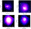 |
Fig. 7. Large-scale Chandra images of A496. (a) Chandra 0.5–4 keV image of the central 60 kpc × 60 kpc region of A496, smoothed with a |

To examine the innermost 70 kpc structures in more detail, we produced an unsharp masked image by smoothing the 0.5–7 keV Chandra images with two Gaussians of σ = 2″ and σ = 10″. The subtraction of the lightly smoothed image from the heavily smoothed one produced the unsharp masked image shown in Fig. 8. The unsharp masked image highlights the large deficit identified in Fig. 7b that is filled by the NE outer lobe. This suggests that the X-ray deficit is an X-ray cavity. Upon inspection, the deficit displays a mushroom-head-shaped morphology, which is also strikingly consistent with the morphology of the radio lobe detected at 330 MHz (red contours in panel b; see also Fig. 3a). Theoretical arguments predict X-ray cavities to assume a torus or mushroom-head shape while buoyantly rising through the cluster potential. As the bubble rises, a trunk of dense gas is entrained in its wake, which penetrates it from below and gives it a mushroom shape (e.g., Gardini 2007). Interestingly, this is consistent with the morphology we observe, as there is a region of enhanced X-ray emission immediately “behind” the cavity that may represent the entrained wake (see Figs. 7b, 8). As visible in Fig. 8b, two additional X-ray depressions are clearly coincident with the inner radio lobes detected at 340 MHz. These features are thus interpreted as real cavities created by displacement of the thermal gas by the inner radio lobes. By comparing the X-ray surface brightness inside and surrounding the cavities (Eqs. (1) and (2) in Ubertosi et al. 2021), we find that the inner depressions represent 15% deficits at a signal-to-noise ratio (S/N) of about 4.9, while the outer bubble represents a 7% deficit at S/N = 3.8. We do not detect an X-ray cavity at the position of the western outer lobe; this could be caused by a combination of projection effects and the influence of the external medium. The western outer lobe is less extended than the eastern one, which suggests it is more strongly projected along the line of sight. The western outer lobe also lies along the brighter part of the X-ray sloshing spiral, pointing to a contribution of bulk motions of the surrounding gas in bending the lobe towards the line of sight. As the contrast of the X-ray cavity decreases with increasing distance from the plane of the sky, projection effects may be hiding any X-ray cavity associated with the western outer lobe.
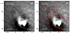 |
Fig. 8. Mushroom-head-shaped X-ray cavity in A496. (a) Chandra unsharp masked image of A496, obtained by subtracting a 10″σ smoothed image from a 2″σ smoothed one. The image has been further smoothed with a 4″σ Gaussian. (b) Same as panel (a), with red contours from the GMRT at 330 MHz at levels of 1.5, 3, 6, and 12 mJy/beam. Green contours are from the VLITE at 340 MHz at levels of 2, 4, 8, 16, 32, 64, and 128 mJy/beam. The dashed white region shows the mushroom-head-shaped cavity. |
In Fig. 9 we show the Hα-line intensity image (panel a) from the MUSE data alongside the Chandra unsharp masked image with Hα and 340 MHz contours (panel b). As previously reported black(McDonald et al. 2010; Hamer et al. 2016; Olivares et al. 2023), there is a nebula of warm gas at 104 K surrounding the cD galaxy of A496; the nebula is composed of a bright central region coincident with the position of the radio core; several filaments of about 10 kpc in length extend toward the east, and a third, thin, and faint filament extends toward the NE. From the X-ray/Hα comparison shown in panel (b), we see a significant spatial overlap between the filaments and the regions of enhanced X-ray emission that likely trace denser (and cooler) gas. This is particularly evident along the X-ray-bright ridge that extends eastward from the radio core. The warm gas is structured around the northern inner cavity blackand the corresponding lobe, with the outermost filament circumventing the X-ray depression and heading further north. Due to the limitations in the blackField of view (FoV) of the MUSE data (coincident with the FoV of Fig. 9a), we are unable to tell if the filaments are even more extended. The average velocity dispersion of the filaments along the ridge is σv = 94 ± 5 km/s, whereas that along the thin outer filament is σv = 65 ± 5 km/s. The decreasing velocity dispersion with increasing distance from the center may be consistent with the jets and possibly the ICM bulk motions being able to inject more kinetic energy into the central region (see Olivares et al. 2019). However, a superposition of several unrelated structures with different velocities at the center of the nebula may also explain the higher central velocity dispersion.
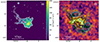 |
Fig. 9. Interaction between the warm gas, the ICM, and the radio source in A496. (a) MUSE image of the Hα line intensity, with overlaid white contours. (b) Chandra unsharp masked image of A496, obtained by subtracting a 10″σ smoothed image from a 2″σ smoothed one. Green contours are from the VLITE at 340 MHz at levels of 2, 4, 8, 16, 32, 64, and 128 mJy/beam, while black contours are from panel (a). Dashed cyan ellipses show the positions of the cavities excavated by the inner lobes (see Sect. 6). |
7. Discussion
7.1. Cycling of the central AGN
Over the three visible outbursts in A496 (compact component, inner lobes, outer lobes), the NE-SW direction of propagation of the jets has remained nearly unchanged. At frequencies of ≳1 GHz, the central radio source contains a bright core, with a possibly inverted spectrum, and two-sided jets extending for about 4 pc in the NE-SW direction (as shown by Ubertosi et al. 2024). On kpc scales, radio lobes are visible to the NE and SW of the core, with a steep radio spectrum and a total synchrotron age of about 26 Myr (see Sect. 5.3). These lobes are associated with X-ray cavities (Fig. 9), indicating that the jets have pushed aside the gas during their propagation. Two larger-scale fossil radio lobes emerge at lower frequency, located approximately along the same axis as the inner lobes, and their shape appears to slightly bend in the same direction. Our analysis indicates that the outer lobes possess an ultrasteep radio spectrum, as typical of fading radio lobes produced in an earlier phase of activity. Chandra images show a large surface-brightness depression at the location of the NE outer lobe (Fig. 8b), suggesting that this region has likely been emptied of its X-ray gas by the expanding radio bubble (see Sect. 6).
As noted in Sect. 5.3, we are only able to approximate the synchrotron ages of the outer lobes, finding a timescale of ∼50 − 300 Myr. An alternative method to estimate the age of the oldest outburst consists in deriving the age of the cavity associated with the NE outer lobe from the X-ray data. Given the diffuse, detached, and clearly buoyant morphology of the outer cavity, we derive its age using the buoyancy timescale (e.g., Bîrzan et al. 2004):
 (2)
(2)
where Dcav, V, and S are the distance from the center, the volume, and the surface area of the cavity, respectively, while g is the gravitational acceleration at the cavity position. To describe the geometry of the cavity (Fig. 8), we considered a sphere with a radius of 13 kpc at 33 kpc from the center (the bubble), from which we subtract another sphere with a radius of 6 kpc at 26 kpc from the center (the wake). While this is a relatively simple approximation of the complex mushroom-wake morphology, we estimate that the impact on the final result (driven by  in Eq. (2)) is limited to ≤20%, which we assume as our uncertainty. We measured the gravitational acceleration at the cavity position from the mass profile determined in Pulido et al. (2018), which accounts for the potential of the dark matter and of the cD galaxy, finding g = 4.9 × 10⁻⁸ cm s−2.
Using Eq. (2), we find that the buoyant rise time of the cavity associated with the NE outer lobe is tb = 45 ± 9 Myr. This is longer than the total synchrotron age of the inner lobes (26 ± 4 Myr), supporting the idea that the outer lobes are the oldest. Furthermore, projection effects may bias the tb estimated above towards shorter timescales than the real ones.
7.2. Cooling of the ICM
Below the mushroom-shaped bubble, an elongated trail of X-ray-bright gas is visible. Two scenarios can explain the formation of this trail in the X-ray map. Based on Fig. 7b, the X-ray-bright gas extends from the cold front south of the central galaxy toward the northeast. Thus, it is possible that the trail is an extension of this cold front, consisting of ICM that is oscillating in the potential of the cluster. Closer to the center, the ridge connecting the trail feature to the central galaxy may represent a stem of cool gas that is experiencing ram pressure from the hotter gas (see, for comparison, Fig. 7 in Ascasibar & Markevitch 2006). Similarly, the structure of the Hα filaments (Fig. 10b) may have been generated by the same sloshing-induced motions. Alternatively, the X-ray trail and the corresponding Hα filaments may be related to the rising mushroom-head cavity. Simulations of the uprising of X-ray cavities show that compression of the ICM entrained by the bubbles in their wake increases the cooling rate, thus generating colder material black(Gardini 2007; Brighenti et al. 2015; Zhang et al. 2022). With time, the lower part of the trunk falls back to the cluster center, while the upper part remains at large radii. The shape of the X-ray wake in A496 is consistent with this picture, and the MUSE data provide further support. As visible in Fig. 10, the warm-gas filaments encompass the north inner bubble, and stretch toward the mushroom-shaped cavity. Thus, it is possible that at least part of the warm gas may be the end product of ICM cooling in the wake of the buoyant bubble.
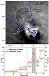 |
Fig. 10. ICM cooling in the wake of the mushroom-head-shaped cavity of A496. Top: Chandra unsharp masked image of A496, as shown in Fig. 8. Black contours show the morphology and extent of the warm gas nebula. The position of the wake of entrained gas is highlighted by arrows. The blue lines represent the sector used to extract the radial profiles of cooling instabilities shown in the bottom panel, and the blue arc shows the maximum extent of Hα filaments. The dashed white region shows the mushroom-head-shaped cavity. Bottom: radial profiles of tcool/tff (in green) and tcool/teddy (in orange) across the blue sector shown in the top panel. The blue vertical line marks the maximum extent of the detected Hα filaments, while the gray-shaded area represents the radial extent of the outer X-ray cavity. We note that the profiles in the bottom panel are plotted further out than the extent of the blue sector in the top panel. |
Different observational strategies have been proposed to verify if the cooling of the hot gas is efficient enough to stimulate the condensation into warm gas filaments. A ratio of ≤20 − 30 between the cooling time tcool and the free-fall time tff (e.g., Voit & Donahue 2015) has been proposed as a sensitive predictor of the radial range over which cooling is expected to occur. Alternatively, Gaspari et al. (2018) proposed that cooling instabilities are expected to develop when the ratio between the cooling time and the eddy turnover time, teddy (i.e., the time at which a turbulent vortex gyrates and produces density fluctuations), is ⪅1. We tested these ratios in A496 by deriving the radial profiles of the above quantities (tcool, tff, teddy) in a narrow wedge (50° wide) centered on the radio core and encompassing the X-ray-bright wake (see Fig. 10). The radial bins were chosen to collect at least 4000 net counts in the 0.5–7 keV band per bin. We derived the following:
-
The cooling time profile. By fitting a projct*tbabs*apec model using XSPEC to the spectra of the radial bins, we derived the deprojected temperature kT and electron density ne of the ICM. We then measured the cooling time as:
 (3)
(3)where γ = 5/3 is the adiabatic index, μ ≈ 0.6 is the mean molecular weight, X ≈ 0.7 is the hydrogen mass fraction, and Λ(T,Z) is the cooling function (from Sutherland & Dopita 1993). We find that the cooling time has its minimum of tcool = 370 ± 23 Myr in the innermost bin (r ≤ 8 kpc).
-
Free-fall time profile. The free fall time is defined as:
 (4)
(4)where g(r) is the gravitational acceleration at a distance of r. We measured g(r) from the mass profile determined in Pulido et al. (2018).
-
Eddy turnover time profile. The eddy turnover time is defined as:
 (5)
(5)where L is the injection scale of turbulence (usually assumed to be described by the extent of the warm gas filaments), and σv,3D is the 3D velocity dispersion of the gas (Gaspari et al. 2018). We measured the teddy profile in the concentric wedges assuming L = 20 kpc (the length of the Hα-filaments; see Fig. 9), and using
 km/s measured from MUSE data.
Figure 10 (bottom) shows the resulting radial profiles of tcool/tff and tcool/teddy. Both cooling thresholds are met up to the maximum extent of the filaments, as similarly found in studies of larger samples of clusters and groups (e.g., Olivares et al. 2019). The profiles steeply rise outwards, indicating that cooling becomes less efficient with increasing radius. However, we note that the fourth radial bin, at 20 ≤ r ≤ 33 kpc, shows tcool/tff = 29 and tcool/teddy = 2, which are close to the cooling thresholds. Thus, warm gas might be trailing the mushroom-head-shaped cavity along the full length of the wake.
Only future optical IFU observations with a larger FoV (e.g., with SITELLE, Grandmont et al. 2012) or with an offset pointing (e.g., with MUSE) will be able to reveal any faint warm gas filament extending all the way to the tip of the wake behind the mushroom-head-shaped cavity. This kind of configuration has only so far been revealed in the case of the Perseus cluster. In that case, the warm gas filaments behind the NW buoyant bubble have a clear horseshoe morphology, since the filaments bend in opposite directions either side of the center of the bubble. The horseshoe filaments may be tracing the toroidal flow pattern induced by the NW bubble of Perseus in its wake (e.g., Fabian et al. 2003; Hatch et al. 2006; Vigneron et al. 2024). Collecting similar morphological and kinematical information for A496 will provide further constraints on cooling instabilities, and will reveal whether the cooling of the ICM into warm gas was stimulated by the uprising of the mushroom-head cavity or by the sloshing motion.
7.3. Nondetection of a mini-halo in A496
In several cool core galaxy clusters, it is possible to observe diffuse radio sources referred to as mini-halos. These extend over the whole cool core region. Radio mini-halos are faint, diffuse, and often associated with sloshing clusters (e.g., ZuHone et al. 2013; Gitti et al. 2018; Giacintucci et al. 2019; Biava et al. 2024). Moreover, the boundary of mini-halos seem to align with cold fronts in the ICM, suggesting that the turbulence generated by the sloshing might energize the relativistic particles traced by their synchrotron emission. Despite ongoing vigorous gas sloshing, and the presence of a favorable source of seed electrons (the central radio galaxy), current radio observations fail to detect a mini-halo in A496. It is likely that the sensitivity and uv coverage of the available images are inadequate to detect very faint diffuse radio emission.
Giacintucci et al. (2019) provided a relation between the 1.4 GHz luminosity of mini-halos and the X-ray luminosity of the ICM within the central 70 kpc. Based on this relation, we can estimate the expected level of diffuse radio emission if A496 were to contain a mini-halo. From the Chandra data, we measure an X-ray bolometric luminosity of 1.2 × 1044 erg s−1 for the inner 70 kpc of A496. From the best-fit relations of Giacintucci et al. (2019), we estimate a 1.4 GHz radio power of about 2 × 10²² − 4 × 10²² W Hz−1, which translates into a flux density of ∼10 − 20 mJy. For comparison, using the relation of Richard-Laferrière et al. (2020) between the 1.4 GHz mini-halo power and the X-ray luminosity within 600 kpc, we would expect a radio power of about 1023 W Hz−1. Thus, the relation of Giacintucci et al. (2019) provides the most stringent limit. If the above putative flux of ∼10 − 20 mJy were uniformly spread over the innermost 70 kpc (which is also the distance of the northern cold front from the center), we would expect an average surface brightness of ∼0.3 − 0.6 μJy/arcsec2 at 1.4 GHz, of ∼0.7 − 1.4 μJy/arcsec2 at 617 MHz, and of ∼1.3 − 2.6 μJy/arcsec2 at 330 MHz (assuming a spectral index α = 1). These estimates demonstrate the current nondetectability of a mini-halo, since such faint emission is well below the sensitivity of the available radio images (4 μJy/arcsec2 at 330 MHz, 12 μJy/arcsec2 at 617 MHz).
8. Summary
In this work, we presented deep, multifrequency radio images of the cool core cluster A496, which allowed us to detect three distinct jet episodes. On subkpc scales, there is evidence of an ongoing SMBH activity with a possibly inverted radio spectrum (α ∼ 0.7 above 5 GHz and α ∼ 0 below). On scales of ∼20 kpc, an blackolder SMBH activity inflated radio lobes with a steep spectral index (α = 2.0 ± 0.1). Our modeling of their synchrotron spectrum indicates that the jet activity lasted for ∼20 Myr before switching off about 6 Myr ago. On larger scales (∼50 − 100 kpc), the GMRT images reveal an blackeven older episode of activity with an ultrasteep spectrum (α = 2.7 ± 0.2).
The archival Chandra data reveal X-ray cavities corresponding to the lobes of the older activity, and to the northeastern lobe of the oldest activity. The outer cavity has the shape of a mushroom head, which is typical of late-time buoyant motions of bubbles. Based on the buoyancy timescale, we estimate a travel time of ∼45 Myr. Furthermore, there is an X-ray-bright feature trailing the fossil lobe or cavity, along which the hot gas has efficiently cooled. Indeed, warm gas filaments traced by their Hα emission are seen stretching toward the northeastern outer bubble. Condensation of the ICM may have been stimulated by the rising cavity in its wake, or by uplift due to sloshing motions. The first scenario will be supported if future optical IFU observations with an offset pointing or with a larger FoV reveal that warm filaments extend to the tip of the wake.
Despite the vigorous sloshing occurring in A496, our radio images fail to detect a radio mini-halo within the cool core. Based on scaling relations between the radio power of mini-halos and the X-ray luminosity of the host cool core, we estimate that a sensitivity of between ∼0.3 and 3 μJy/arcsec2 (depending on frequency) – which is well below that of the radio images presented in this work – would be required to detect the faint, diffuse emission. Future observations with the upgraded GMRT, the JVLA, or the Square Kilometer Array precursors ASKAP and MeerKAT may provide the sensitivity and uv coverage needed to unveil an extremely faint mini-halo in this sloshing cool core, further supporting the connection between sloshing and mini-halo formation, and extending it down to smaller host-cluster masses.
An image at 150 MHz from the same data sets as those analyzed here is available from the TIFR GMRT Sky Survey Alternative Data Release (TGSS-ADR, Intema et al. 2017), where the radio source is detected with a similar morphology and flux density as measured in our image.
We assumed a filling factor of 1 and zero protons (k = 0).
Acknowledgments
We thank the anonymous reviewer for their useful comments to our manuscript. Basic research in radio astronomy at the Naval Research Laboratory is supported by 6.1 Base funding. Construction and installation of VLITE was supported by the NRL Sustainment Restoration and Maintenance fund. The National Radio Astronomy Observatory is a facility of the National Science Foundation operated under cooperative agreement by Associated Universities, Inc. The scientific results reported in this article are based on data obtained from the GMRT Data Archive. We thank the staff of the GMRT that made the observations possible. GMRT is run by the National Centre for Astrophysics of the Tata Institute of Fundamental Research. This scientific work makes use of the data from the Murchison Radio-astronomy Observatory and Australian SKA Pathfinder, managed by CSIRO. Support for the operation of the MWA and ASKAP is provided by the Australian Government (NCRIS). ASKAP and MWA use the resources of the Pawsey Supercomputing Centre. Establishment of ASKAP, MWA and the Pawsey Supercomputing Centre are initiatives of the Australian Government, with support from the Government of Western Australia and the Science and Industry Endowment Fund. We acknowledge the Wajarri Yamatji people as the traditional owners of the observatory sites. This paper employs a list of Chandra datasets, obtained by the Chandra X-ray Observatory, contained in the Chandra Data Collection (CDC) https://doi.org/10.25574/cdc.241. This research has made use of software provided by the Chandra X-ray Center (CXC) in the application packages CIAO. The results are based on observations collected at the European Southern Observatory under ESO programme 094.B-059.
References
- Andernach, H., Han, T., Sievers, A., et al. 1988, A&AS, 2, 265 [NASA ADS] [Google Scholar]
- Ascasibar, Y., & Markevitch, M. 2006, ApJ, 650, 102 [Google Scholar]
- Asplund, M., Grevesse, N., Sauval, A. J., et al. 2009, ARA&A, 47, 481 [Google Scholar]
- Biava, N., Bonafede, A., Gastaldello, F., et al. 2024, A&A, 686, A82 [NASA ADS] [CrossRef] [EDP Sciences] [Google Scholar]
- Bîrzan, L., Rafferty, D. A., McNamara, B. R., et al. 2004, ApJ, 607, 800 [CrossRef] [Google Scholar]
- Bourne, M. A., & Yang, H.-Y. K. 2023, Galaxies, 11, 73 [NASA ADS] [CrossRef] [Google Scholar]
- Briggs, D. S. 1995, Ph.D. Thesis, New Mexico Institute of Mining and Technology, USA [Google Scholar]
- Brighenti, F., Mathews, W. G., & Temi, P. 2015, ApJ, 802, 118 [NASA ADS] [CrossRef] [Google Scholar]
- Brinchmann, J., Charlot, S., White, S. D. M., et al. 2004, MNRAS, 351, 1151 [Google Scholar]
- CASA Team (Bean, B., et al.) 2022, PASP, 134, 114501 [NASA ADS] [CrossRef] [Google Scholar]
- Chandra, P., Ray, A., & Bhatnagar, S. 2004, ApJ, 612, 974 [Google Scholar]
- Churazov, E., Brüggen, M., Kaiser, C. R., et al. 2001, ApJ, 554, 261 [NASA ADS] [CrossRef] [Google Scholar]
- Clarke, T. E., Perley, R. A., Kassim, N. E., et al. 2011, Gen. Assem. Sci. Symp., E5 [Google Scholar]
- Clarke, T. E., Kassim, N. E., Brisken, W., et al. 2016, Proc. SPIE, 9906, 99065B [NASA ADS] [CrossRef] [Google Scholar]
- Cotton, W. D. 2008, PASP, 120, 439 [Google Scholar]
- Deller, A. T., Tingay, S. J., Bailes, M., et al. 2007, PASP, 119, 318 [NASA ADS] [CrossRef] [Google Scholar]
- Dupke, R., & White, R. E. 2003, ApJ, 583, L13 [NASA ADS] [CrossRef] [Google Scholar]
- Dupke, R., White, R. E., & Bregman, J. N. 2007, ApJ, 671, 181 [NASA ADS] [CrossRef] [Google Scholar]
- Eilek, J. A. 2014, New J. Phys., 16, 045001 [NASA ADS] [CrossRef] [Google Scholar]
- Fabian, A. C., Sanders, J. S., Crawford, C. S., et al. 2003, MNRAS, 344, L48 [NASA ADS] [CrossRef] [Google Scholar]
- Fruscione, A., McDowell, J. C., Allen, G. E., et al. 2006, Proc. SPIE, 6270, 62701V [Google Scholar]
- Gardini, A. 2007, A&A, 464, 143 [NASA ADS] [CrossRef] [EDP Sciences] [Google Scholar]
- Gaspari, M., McDonald, M., Hamer, S. L., et al. 2018, ApJ, 854, 167 [Google Scholar]
- Ghizzardi, S., De Grandi, S., & Molendi, S. 2014, A&A, 570, A117 [NASA ADS] [CrossRef] [EDP Sciences] [Google Scholar]
- Giacintucci, S., Markevitch, M., Cassano, R., et al. 2019, ApJ, 880, 70 [Google Scholar]
- Gitti, M., Brunetti, G., Cassano, R., et al. 2018, A&A, 617, A11 [NASA ADS] [CrossRef] [EDP Sciences] [Google Scholar]
- Govoni, F., & Feretti, L. 2004, Int. J. Mod. Phys. D, 13, 1549 [Google Scholar]
- Grandmont, F., Drissen, L., Mandar, J., et al. 2012, Proc. SPIE, 8446, 84460U [NASA ADS] [CrossRef] [Google Scholar]
- Greisen, E. W. 2003, Inf. Handling Astron. - Historical Vistas, 285, 109 [NASA ADS] [CrossRef] [Google Scholar]
- Hale, C. L., McConnell, D., Thomson, A. J. M., et al. 2021, PASA, 38, e058 [NASA ADS] [CrossRef] [Google Scholar]
- Hamer, S. L., Edge, A. C., Swinbank, A. M., et al. 2016, MNRAS, 460, 1758 [Google Scholar]
- Hardcastle, M. J., & Croston, J. H. 2020, New A Rev., 88, 101539 [NASA ADS] [CrossRef] [Google Scholar]
- Hatch, N. A., Crawford, C. S., Johnstone, R. M., et al. 2006, MNRAS, 367, 433 [CrossRef] [Google Scholar]
- HI4PI Collaboration (Ben Bekhti, N., et al.) 2016, A&A, 594, A116 [NASA ADS] [CrossRef] [EDP Sciences] [Google Scholar]
- Hogan, M. T., Edge, A. C., Hlavacek-Larrondo, J., et al. 2015a, MNRAS, 453, 1201 [NASA ADS] [CrossRef] [Google Scholar]
- Hogan, M. T., Edge, A. C., Geach, J. E., et al. 2015b, MNRAS, 453, 1223 [NASA ADS] [CrossRef] [Google Scholar]
- Hurley-Walker, N., Callingham, J. R., Hancock, P. J., et al. 2017, MNRAS, 464, 1146 [Google Scholar]
- Intema, H. T., van der Tol, S., Cotton, W. D., et al. 2009, A&A, 501, 1185 [NASA ADS] [CrossRef] [EDP Sciences] [Google Scholar]
- Intema, H. T., Jagannathan, P., Mooley, K. P., et al. 2017, A&A, 598, A78 [NASA ADS] [CrossRef] [EDP Sciences] [Google Scholar]
- Kaiser, C. R., Pavlovski, G., Pope, E. C. D., et al. 2005, MNRAS, 359, 493 [NASA ADS] [CrossRef] [Google Scholar]
- Lacy, M., Baum, S. A., Chandler, C. J., et al. 2020, PASP, 132, 035001 [Google Scholar]
- Lane, W. M., Cotton, W. D., van Velzen, S., et al. 2014, MNRAS, 440, 327 [Google Scholar]
- McConnell, D., Hale, C. L., Lenc, E., et al. 2020, PASA, 37, e048 [Google Scholar]
- McDonald, M., Veilleux, S., Rupke, D. S. N., et al. 2010, ApJ, 721, 1262 [NASA ADS] [CrossRef] [Google Scholar]
- McNamara, B. R., & Nulsen, P. E. J. 2007, ARA&A, 45, 117 [NASA ADS] [CrossRef] [Google Scholar]
- McNamara, B. R., & Nulsen, P. E. J. 2012, New J. Phys., 14, 055023 [NASA ADS] [CrossRef] [Google Scholar]
- Murgia, M., Parma, P., Mack, K.-H., et al. 2011, A&A, 526, A148 [NASA ADS] [CrossRef] [EDP Sciences] [Google Scholar]
- Noordam, J. E. 2004, Proc. SPIE, 5489, 817 [NASA ADS] [CrossRef] [Google Scholar]
- O’Dea, C. P., & Saikia, D. J. 2021, A&ARv, 29, 3 [Google Scholar]
- Offringa, A. R., & Smirnov, O. 2017, MNRAS, 471, 301 [Google Scholar]
- Offringa, A. R., McKinley, B., Hurley-Walker, N., et al. 2014, MNRAS, 444, 606 [Google Scholar]
- Olivares, V., Salome, P., Combes, F., et al. 2019, A&A, 631, A22 [NASA ADS] [CrossRef] [EDP Sciences] [Google Scholar]
- Olivares, V., Su, Y., Forman, W., et al. 2023, ApJ, 954, 56 [NASA ADS] [CrossRef] [Google Scholar]
- Perley, R. A., & Butler, B. J. 2017, ApJS, 230, 7 [NASA ADS] [CrossRef] [Google Scholar]
- Planck Collaboration XXIX. 2014, A&A, 571, A29 [NASA ADS] [CrossRef] [EDP Sciences] [Google Scholar]
- Polisensky, E., Lane, W. M., Hyman, S. D., et al. 2016, ApJ, 832, 60 [NASA ADS] [CrossRef] [Google Scholar]
- Pulido, F. A., McNamara, B. R., Edge, A. C., et al. 2018, ApJ, 853, 177 [NASA ADS] [CrossRef] [Google Scholar]
- Quici, B., Turner, R. J., Seymour, N., et al. 2022, MNRAS, 514, 3466 [NASA ADS] [CrossRef] [Google Scholar]
- Reynolds, C. S., McKernan, B., Fabian, A. C., et al. 2005, MNRAS, 357, 242 [NASA ADS] [CrossRef] [Google Scholar]
- Richard-Laferrière, A., Hlavacek-Larrondo, J., Nemmen, R. S., et al. 2020, MNRAS, 499, 2934 [Google Scholar]
- Roediger, E., Lovisari, L., Dupke, R., et al. 2012, MNRAS, 420, 3632 [CrossRef] [Google Scholar]
- Roediger, E., Kraft, R. P., Nulsen, P., et al. 2013, MNRAS, 436, 1721 [Google Scholar]
- Scaife, A. M. M., & Heald, G. H. 2012, MNRAS, 423, L30 [Google Scholar]
- Sijacki, D., & Springel, V. 2006, MNRAS, 371, 1025 [NASA ADS] [CrossRef] [Google Scholar]
- Stanghellini, C., O’Dea, C. P., Baum, S. A., et al. 1997, A&A, 325, 943 [Google Scholar]
- Sutherland, R. S., & Dopita, M. A. 1993, ApJS, 88, 253 [Google Scholar]
- Tanaka, T., Kunieda, H., Hudaverdi, M., et al. 2006, PASJ, 58, 703 [NASA ADS] [CrossRef] [Google Scholar]
- Tremonti, C. A., Heckman, T. M., Kauffmann, G., et al. 2004, ApJ, 613, 898 [Google Scholar]
- Ubertosi, F., Gitti, M., Brighenti, F., et al. 2021, ApJ, 923, L25 [NASA ADS] [CrossRef] [Google Scholar]
- Ubertosi, F., Schellenberger, G., O’Sullivan, E., et al. 2024, ApJ, 961, 134 [CrossRef] [Google Scholar]
- Vigneron, B., Hlavacek-Larrondo, J., Rhea, C. L., et al. 2024, ApJ, 962, 96 [NASA ADS] [CrossRef] [Google Scholar]
- Voit, G. M., & Donahue, M. 2015, ApJ, 799, L1 [NASA ADS] [CrossRef] [Google Scholar]
- Wang, Q. H. S., Markevitch, M., & Giacintucci, S. 2016, ApJ, 833, 99 [NASA ADS] [CrossRef] [Google Scholar]
- Weilbacher, P. M., Streicher, O., Urrutia, T., et al. 2014, ASP Conf. Ser., 485, 451 [NASA ADS] [Google Scholar]
- Zhang, C., Zhuravleva, I., Gendron-Marsolais, M.-L., et al. 2022, MNRAS, 517, 616 [CrossRef] [Google Scholar]
- ZuHone, J. A., Markevitch, M., Brunetti, G., et al. 2013, ApJ, 762, 78 [NASA ADS] [CrossRef] [Google Scholar]
All Tables
All Figures
|
Fig. 1. VLA A–configuration image at 1.5 GHz (blue and contours) of the central radio source in A496, overlaid on the optical HST WFPC2 image of the central galaxy (orange). The restoring beam of the radio image is 2″ × 1″, at a position angle (PA) of 17° (boxed white ellipse in the bottom left corner) and the noise level is 1σ = 50 μJy beam−1. Contours are spaced by a factor of 2 starting from +3σ. |
| In the text | |
|
Fig. 2. Radio images of the inner source in A496. (a): VLITE 340 MHz image. The beam is 7″ × 4″, in PA −2° and noise is 1σ = 0.66 mJy/beam. (b): GMRT 617 MHz image. The beam is 6″ × 5″, in PA −54° and 1σ = 0.47 mJy/beam. (c): VLA–B configuration combined image at 1.4 GHz. The image has been restored with a 5″ circular beam. The noise is 1σ = 0.1 mJy/beam. (d): VLA–C configuration image at 4.7 GHz. The image has been restored with a 4″ circular beam. The noise is 1σ = 0.03 mJy/beam. In all panels, contours are spaced by a factor of 2 starting from +3σ. Contours at −3σ mJy/beam are shown as dashed lines. The boxed ellipse or circle shows the beam size. The white cross marks the optical peak (Fig. 1). In panel (a), the magenta box is as in Fig. 3. |
| In the text | |
|
Fig. 3. Radio images of the outer radio lobes in A496. (a): GMRT image at 330 MHz (grayscale and contours). The image has been restored with a 12″ circular beam and the noise is 1σ = 0.5 mJy/beam. (b): GMRT combined image at 150 MHz (grayscale and contours). The restoring beam is 24″ × 18″, in PA 0° and 1σ = 10 mJy/beam. In both panels, contours are spaced by a factor of 2 starting from +3σ. No contours at −3σ are present in the portion of the image shown. The boxed ellipse or circle shows the beam size. The magenta box marks the area occupied by the inner double source (see Fig. 2a). The white cross marks the optical peak (Fig. 1). |
| In the text | |
|
Fig. 4. Spectra of the radio source at the center of A496. Left: integrated radio spectrum of the total radio emission at the center of A496. Our flux density measurements are shown as purple filled squares. Catalog and literature values from Table 4 are shown in black. Right: radio spectra of the individual components. The blue dashed line shows the spectral slope of the outer lobes. The dashed pink line and shaded area represent the best fit and associated uncertainty with a CI-off model to the spectrum of the inner lobes. The VLBA 5 GHz flux density from Ubertosi et al. (2024) is plotted with a gold circle. |
| In the text | |
|
Fig. 5. VLBA image at 5 GHz of the compact component in A496 at a resolution of 3.5 × 1.2 mas and with noise of σ = 60 μJy/beam. Contours start at 5σ and increase by a factor of 2. |
| In the text | |
|
Fig. 6. Color-scale image of the spectral index distribution between 150 MHz and 330 MHz (a) and the associated error map (b), computed from primary-beam-corrected images with the same uv range and beam of 24″ × 18″. The spectral index was calculated in each pixel where the surface brightness is above the 3σ level in both images. Overlaid are the 330 MHz contours, spaced by a factor of 2 from 3σ = 3 mJy/beam. The white box marks the region occupied by the inner double source (Fig. 2a). The white cross marks the optical peak (Fig. 1). |
| In the text | |
|
Fig. 7. Large-scale Chandra images of A496. (a) Chandra 0.5–4 keV image of the central 60 kpc × 60 kpc region of A496, smoothed with a |
| In the text | |
|
Fig. 8. Mushroom-head-shaped X-ray cavity in A496. (a) Chandra unsharp masked image of A496, obtained by subtracting a 10″σ smoothed image from a 2″σ smoothed one. The image has been further smoothed with a 4″σ Gaussian. (b) Same as panel (a), with red contours from the GMRT at 330 MHz at levels of 1.5, 3, 6, and 12 mJy/beam. Green contours are from the VLITE at 340 MHz at levels of 2, 4, 8, 16, 32, 64, and 128 mJy/beam. The dashed white region shows the mushroom-head-shaped cavity. |
| In the text | |
|
Fig. 9. Interaction between the warm gas, the ICM, and the radio source in A496. (a) MUSE image of the Hα line intensity, with overlaid white contours. (b) Chandra unsharp masked image of A496, obtained by subtracting a 10″σ smoothed image from a 2″σ smoothed one. Green contours are from the VLITE at 340 MHz at levels of 2, 4, 8, 16, 32, 64, and 128 mJy/beam, while black contours are from panel (a). Dashed cyan ellipses show the positions of the cavities excavated by the inner lobes (see Sect. 6). |
| In the text | |
|
Fig. 10. ICM cooling in the wake of the mushroom-head-shaped cavity of A496. Top: Chandra unsharp masked image of A496, as shown in Fig. 8. Black contours show the morphology and extent of the warm gas nebula. The position of the wake of entrained gas is highlighted by arrows. The blue lines represent the sector used to extract the radial profiles of cooling instabilities shown in the bottom panel, and the blue arc shows the maximum extent of Hα filaments. The dashed white region shows the mushroom-head-shaped cavity. Bottom: radial profiles of tcool/tff (in green) and tcool/teddy (in orange) across the blue sector shown in the top panel. The blue vertical line marks the maximum extent of the detected Hα filaments, while the gray-shaded area represents the radial extent of the outer X-ray cavity. We note that the profiles in the bottom panel are plotted further out than the extent of the blue sector in the top panel. |
| In the text | |
Current usage metrics show cumulative count of Article Views (full-text article views including HTML views, PDF and ePub downloads, according to the available data) and Abstracts Views on Vision4Press platform.
Data correspond to usage on the plateform after 2015. The current usage metrics is available 48-96 hours after online publication and is updated daily on week days.
Initial download of the metrics may take a while.