| Issue |
A&A
Volume 691, November 2024
Solar Orbiter First Results (Nominal Mission Phase)
|
|
|---|---|---|
| Article Number | A77 | |
| Number of page(s) | 17 | |
| Section | The Sun and the Heliosphere | |
| DOI | https://doi.org/10.1051/0004-6361/202451272 | |
| Published online | 29 October 2024 | |
Testing the flux tube expansion factor - solar wind speed relation with Solar Orbiter data
1
LESIA, Observatoire de Paris, Université PSL, CNRS, Sorbonne Université, Université de Paris, 5 place Jules Janssen, 92195 Meudon, France
2
IRAP, Observatoire Midi-Pyrénées, Université Toulouse III – Paul Sabatier, CNRS, 9 avenue du Colonel Roche, 31400 Toulouse, France
3
Laboratoire Cogitamus, 75005 Paris, France
⋆ Corresponding author; This email address is being protected from spambots. You need JavaScript enabled to view it.
Received:
26
June 2024
Accepted:
8
August 2024
Abstract
Context. The properties of the solar wind measured in situ in the heliosphere are largely controlled by energy deposition in the solar corona, which is in turn closely related to the properties of the coronal magnetic field. Previous studies have shown that long-duration and large-scale magnetic structures show an inverse relation between the solar wind velocity measured in situ near 1 au and the expansion factor of the magnetic flux tubes in the solar atmosphere.
Aims. The advent of the Solar Orbiter mission offers a new opportunity to analyse the relation between solar wind properties measured in situ in the inner heliosphere and the coronal magnetic field. We exploit this new data in conjunction with models of the coronal magnetic field and the solar wind to evaluate the flux expansion factor and speed relation.
Methods. We use a Parker-like solar wind model, the “isopoly” model presented in previous works, to describe the motion of the solar wind plasma in the radial direction and model the tangential plasma motion due to solar rotation with the Weber and Davis equations. Both radial and tangential velocities are used to compute the plasma trajectory and streamline from Solar Orbiter location sunward to the solar ‘source surface’ at rss. We then employed a potential field source surface (PFSS) model to reconstruct the coronal magnetic field below rss to connect wind parcels mapped back to the photosphere.
Results. We found a statistically weak anti-correlation between the in situ bulk velocity and the coronal expansion factor, for about 1.5 years of solar data. Classification of the data by source latitude reveals different levels of anticorrelation, which is typically higher when Solar Orbiter magnetically connects to high latitude structures than when it connects to low latitude structures. We show the existence of a fast solar wind that originates in strong magnetic field regions at low latitudes and undergoes large expansion factor. We provide evidence that such winds become supersonic during the super-radial expansion (below rss) and are theoretically governed by a positive v–f correlation. We find that faster winds exhibit, on average, a flux tube expansion at a larger radius than slower winds.
Conclusions. An anticorrelation between solar wind speed and expansion factor is present for solar winds originating in high latitude structures in solar minimum activity, typically associated with coronal hole-like structures, but this cannot be generalized to lower latitude sources. We have found extended time intervals of fast solar wind associated with both large expansion factors and strong photospheric magnetic fields. Therefore, the value of the expansion factor alone cannot be used to predict the solar wind speed. Other parameters, such as the height at which the expansion gradient is the strongest, must also be taken into account.
Key words: Sun: atmosphere / Sun: corona / Sun: magnetic fields / solar wind
Publisher note: The article title was corrected on 8 November 2024.
© The Authors 2024
 Open Access article, published by EDP Sciences, under the terms of the Creative Commons Attribution License (https://creativecommons.org/licenses/by/4.0), which permits unrestricted use, distribution, and reproduction in any medium, provided the original work is properly cited.
This article is published in open access under the Subscribe to Open model. This email address is being protected from spambots. You need JavaScript enabled to view it. to support open access publication.
1. Introduction
Decades of heliospheric exploration have attempted to understand the relation between solar wind properties measured in situ and its source in the solar corona (Wang & Sheeley 1990; Neugebauer et al. 1998; Abbo et al. 2016; Bemporad 2017). These properties are defined during the formation of the wind and can evolve greatly during propagation in the interplanetary medium. Measurements taken closer to the wind sources with Solar Orbiter (SolO) and Parker Solar Probe (PSP) allow us to alleviate some of the propagation effects and improve our comparative studies of wind properties with coronal structures.
A large fraction of the open magnetic field lines along which the solar wind originates are rooted in coronal holes clearly visible in ultraviolet solar imaging. These holes only occupy a fraction of the solar photosphere. At solar minimum, coronal holes persist at high latitudes near the poles and cover about 15−20% of the total solar surface area (Bohlin 1977). These polar holes can extend down to a latitude of 60° in each hemisphere (Wang et al. 1996, 2010). As solar activity increases, the area of polar holes shrinks to less than 5% of the total surface area near solar maximum. In contrast to the rather persistent polar holes, these low-latitude holes tend to evolve rapidly in response to solar activity (see, e.g., Broussard et al. 1978; Insley et al. 1995; Dorotovič 1996). This cyclic evolution induces strong topological changes in the magnetic fields and on the solar wind properties as a result.
Since open field lines only occupy a small fraction of the total solar surface, magnetic equilibrium will force solar wind flux tubes to expand faster than predicted by a simple spherical expansion (Zirker 1977). This super-radial expansion is described by the expansion factor, f(r), typically defined as
 (1)
(1)
where Br(r) is the magnetic field radial component at the radial position, r, and r⊙ is the Sun’s radius. Using a magnetic model of the solar corona and an empirical extrapolation of the 1 au velocity v from the f(rss) value computed at the source surface radius rss, Wang & Sheeley (1990) noticed an anticorrelation pattern between the 1 au solar wind velocity v and f(rss) for observations on large spatial and temporal scales. Their analysis used a magnetostatic reconstruction of the solar atmosphere called the potential field source surface (PFSS) model, where the magnetic field is supposed to be potential within r⊙ < r < rss and radial for r > rss. Using a similar approach, Arge & Pizzo (2000) found a better anti-correlation by also considering the distance of the wind source to the closest coronal hole boundary. Other magnetic connectivity studies and magnetohydrodynamic (MHD) simulation studies have looked at different solar sources and their correlation with in situ properties, but these either considered short time intervals or a specific type of magnetic structure (Riley & Luhmann 2012; Pinto et al. 2016; Réville & Brun 2017; Wallace et al. 2020; Badman et al. 2023; Yardley et al. 2024). In addition, the MHD simulation study of Pinto et al. (2016) highlights that discrepancies of the global v–f anticorrelation can exist, supporting that the global scaling law of Arge & Pizzo (2000) requires adjustments. Thus, we cannot say to what extent the v–f anti-correlation can be generalized to all observed solar wind time periods.
Magnetic connectivity mapping is a central step in these studies. The tracing of a spacecraft magnetic connectivity to the photosphere has typically been divided in two spatial domains. Starting from the spacecraft, a magnetic field line is first traced through the interplanetary medium to the upper corona by usually following the nominal “Parker spiral”. In a second step, a model of the complex coronal magnetic field is usually considered to trace magnetic field lines from the upper corona down to the photosphere.
For the first step, a recent study by Dakeyo et al. (2024) compared the different existing mapping methods. While the ballistic backmapping approach (constant wind speed) is the most commonly used, they showed that the best practice remains to consider wind acceleration and corotation effects, especially when studying different wind speed streams. For the second step, past research comparing different coronal models with the PFSS reconstructions conclude that PFSS provides good results, particularly near solar minimum when the large-scale currents are negligible and the source surface can be considered to be nearly spherical (Riley et al. 2006; Arden et al. 2014). The PFSS model uses as input the radial component of the photospheric magnetic field Br(r⊙), provided in the form of photospheric magnetograms. The distribution of Br(r⊙) control the topology of the coronal magnetic field and determine the trajectory followed by magnetic field lines of interest, so the path of the young solar wind as the plasma is frozen in the magnetic field.
Complementary observational constraints can be obtained with in situ measurements. The radial evolution of the thermodynamic properties of the solar wind has been studied by many authors (Schwartz & Marsch 1983; Hellinger et al. 2011, 2013; Štverák et al. 2015; Sanchez-Diaz et al. 2016, 2019; Maksimovic et al. 2020) using the large coverage of heliocentric distances provided by the Helios missions (Porsche 1981). In particular, the study of Maksimovic et al. (2020) has revealed that the slow wind pursues its acceleration at large radial distances (0.3 to 1 au), outside of the main wind acceleration region (≲20 r⊙). Other studies using more recent data from the PSP mission (Fox et al. 2016) have presented similar trends in their conclusions (Halekas et al. 2022; Dakeyo et al. 2022).
Thus, the radial evolution of the velocity beyond the main acceleration region should be accounted for in the solar wind models and should have some influence on our estimates of magnetic field connectivity. In most connectivity studies, the velocity used to model the streamline spiral is assumed to be purely radial and constant with radial distance (e.g., Neugebauer & Snyder 1966; Krieger et al. 1973; Burkholder et al. 2019; Rouillard et al. 2020; Badman et al. 2020; Griton et al. 2021). However, in practice, this is not the case with respect to studies of the radial evolution of the observed wind speed (Maksimovic et al. 2020; Halekas et al. 2022; Dakeyo et al. 2022).
To model the radial evolution of the solar wind speed for different wind types, we have recently developed a simple “isopoly” fluid model (Dakeyo et al. 2022). Derived from a two-fluid Parker-type solar wind model, this approach assumes two different thermal regimes with radial distance: an isothermal corona, representing the region where coronal heating is effective, and a polytropic expansion in the solar wind. This simple model allows for some significant wind acceleration near the Sun (below 15 r⊙), while matching in situ measurements of the radial velocity, temperature and density profiles recorded beyond the solar corona. However, this modeling does not take into account the near-Solar magnetic topology associated with the super-radial expansion.
With all the above concerns in mind, we would like to explore the extent to which the v–f relation could be generalized to different types of solar wind. The context of the Solar Orbiter mission is particularly interesting for a deeper analysis of solar wind properties with radial distance and to improve on current connectivity models (Müller et al. 2020).
In Sect. 2 we aim to perform a statistical study using magnetic connectivity and solar wind modeling. Then, we infer the source location of a large set of in situ measurements made by Solar Orbiter. Given the limitations of existing techniques and models, we have chosen to perform a fast calculation of the near-Sun magnetic topology based on PFSS extrapolation, a refined streamline calculation based on the Parker spiral including isopoly description (radial acceleration) and Weber & Davis (1967) tangential flow (corotational effects). In Sect. 3, we present the magnetic connectivity results on the global v–f induced relation and compare them to the previous results. In Sect. 4, we provide theoretical justification to explain the results. Finally, in Sect. 5, we summarize the main results of our study and discuss their implications on the relation between source and in situ, and global solar wind modeling.
2. Connectivity method and modeling
The magnetic connectivity of a wind streamline was computed as a two-step process, including interplanetary magnetic field modeling and near-Sun magnetic field modeling. We included acceleration and corotational effects in the wind description. Indeed, both can modify the final mapped longitude in the solar corona.
2.1. Radial evolution: IsoPoly equations
Our aim is to model the solar wind evolution with heliocentric distance using in situ measurements from SolO as the upper boundary conditions. Since the model should be run on every available data point of the statistical study, one requirement of our model is to run fast. The “isopoly” fluid model proposed by Dakeyo et al. (2022) fulfills these requirements with short computational time. Moreover, it has already provided a successful description of the solar wind observations of Helios and PSP between 0.1 au and 1 au. The conservation of momentum is:
 (2)
(2)
with n as the density, Ps the plasma pressure, mp the proton mass, and M the Sun’s mass, where the sum over the species, s, is taken over protons (p) and electrons (e). The temperature is
 (3)
(3)
where riso|s is the distance below which the expansion is isothermal, and γs is the polytropic index. The density can be expressed using mass flux conservation, where n u r2 = C, and C is a constant determined from observations. For further information on isopoly equations, we refer to Dakeyo et al. (2022) and Shi et al. (2022).
2.2. Tangential evolution: Weber-Davis equations
In the solar corona, the solar wind initially corotates with the Sun in the inertial frame. Beyond a certain distance, the plasma moves mostly radially at supersonic speeds. The relative rotation between the released plasma and its source creates the Parker spiral pattern (Parker 1958), which is an idealised representation of the magnetic field lines in the interplanetary medium. It corresponds to the velocity streamlines based on the magnetic field lines viewed in the corotating frame (also called the Carrington frame). Throughout this manuscript, the trajectories of the plasma parcels viewed in the solar corotating frame are referred to as streamlines.
In most connectivity studies, the velocity used to model the streamline spiral is assumed to be purely radial and constant with radial distance (e.g., Neugebauer & Snyder 1966; Krieger et al. 1973; Sanchez-Diaz et al. 2016; Rouillard et al. 2020; Badman et al. 2020; Griton et al. 2021). However, in practice, this is not the case as shown in a number of recent studies (Maksimovic et al. 2020; Dakeyo et al. 2022; Halekas et al. 2022). Moreover, even a partial corotation of a solar wind parcel with its source induces a tangential flow, uφ, tightening the streamline and changing the calculated field line trajectory.
Weber & Davis (1967) carried out a study showing for an MHD solar wind outflow that the plasma is almost in quasi-rigid rotation with the Sun very low in the corona (uφ = ΩSun r). The corotation becomes weaker with the radial distance r, especially above the Alfvén critical point, rA, and then tends asymptotically to a non-corotating flow far from the Sun (uφ = 0). This modeling is supported by other recent studies (Macneil et al. 2022; Koukras et al. 2022). Based on a given radial speed profile ur(r), Weber & Davis (1967) derived the following expression for the tangential speed, uφ(r):
 (4)
(4)
where  is the Alfvén speed profile, ρ(r) the total mass density, and MA = ur(r)/uA(r) the Alfvén mach number.
To compute ur(r) we use the five radial isopoly speed profiles of Dakeyo et al. (2022) which are interpolated in order to match the Solar Orbiter in situ bulk speed measurements. From these interpolated profiles, we can compute the associated Alfvén speed uA(r) if we also know the radial evolution of Br provided by Solar Orbiter (detailed later in Sect. 2.3). Using these values and the isopoly density profiles, we can compute the Alfvén speed uA(r). Then, uφ(r) is computed with Eq. (4).
Incorporating uφ in the calculation of the local streamline longitude ϕ based on the expression of the Parker spiral, is achieved by subtracting the relative angular speed of the plasma to ΩSun (Macneil et al. 2022):
 (5)
(5)
where ϕss is the longitude location at rss, and r the distance from which is computed the backmapping. For more details about the tangential speed profiles associated with the isopoly radial solutions, please refer to Dakeyo et al. (2024).
2.3. Solar Orbiter data set and treatment
The three instruments that make up the Solar Wind Analyzer (SWA) suite (Owen et al. 2020) are: Proton-Alpha particle Sensor (PAS), Electron Analyzer System (EAS), and Heavy Ion Sensor (HIS). For the magnetic field data, the magnetometer (MAG) provides 3D measurements of the interplanetary magnetic field (Horbury et al. 2020). Based on the currently available data, we restrict our dataset to the instruments PAS, HIS, and MAG. The Solar Orbiter observations we use for the study cover the period from August 1, 2020 to March 17, 2022. This includes data up to the end of the solar minimum activity period. Since we are not studying short timescales here, we calculated the average values of the observations over 30 minutes to smooth the fast variations and optimize the connectivity process (computation time).
Time intervals for which all the instruments do not provide simultaneous data were not considered and we also removed ICMEs from our Solar Orbiter dataset using the criteria of Elliott et al. (2012). We discarded the measurements for which at least one of the two following criteria on the plasma, β, and the proton temperature, Tp, is satisfied: (i) β < 0.1, (ii) Tp/Tex < 0.5, where Tex is a temperature predicted by the scaling law Tex = 486.5 × u − 1.2476 × 10⁵ K established by Lopez & Freeman (1986), for which Tp is rescaled with solar distance by the solar wind predicted temperature, Tex. We also considered that ICMEs have a duration of at least 6 hours. In addition to these criteria, we removed the 24 h before and 15 h after each detected ICME. Furthermore, we considered wind measurements faster than 800 km/s as potential ICMEs and, thus, we also removed them.
The synchronized and filtered data from Solar Orbiter are shown in Fig. 1. There is a significant data gap between November 2020 and April 2021 because no synchronized data was available for PAS and MAG. This reduces the real observable time to an equivalent of one year of continuous data. However, the wind speed sampling is good enough to assume that the observation depicts a global picture of the solar wind characteristics (apart from an under sampling of the faster winds due to the minimal solar activity).
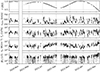 |
Fig. 1. Time series of Solar Orbiter measurements from 1/08/2020 to 17/03/2022 in the period of minimal solar activity. The top panel shows the radial position of SolO. The bulk speed, vwind, proton temperature, Tp, and proton density, np, are provided by the instrument PAS, and the absolute value of the magnetic field radial component, Br, by the instrument MAG. The time intervals for which both instruments do not provide simultaneous data and the observations that are not associated with a complete backmapping process are not displayed. Each data point is a 30 minute average. |
2.4. The PFSS model and magnetograms
The most widely used coronal model is the PFSS, mainly because of its ease of use and short computation time. Above an assumed source surface rss typically placed between 1.5 and 5 r⊙ (most commonly 2.5 r⊙), all field lines are assumed to be open to the interplanetary medium. To determine the trajectory of a given plasma parcel below rss, it is necessary to compute the coronal magnetic equilibrium to determine the open and closed field lines, as well as the complex connectivity. The reconstruction is quite accurate for studying the solar corona near solar minimum, but it neglects the electric current and assumes the magnetic field to be fully potential and is therefore less accurate during active solar periods (Riley et al. 2006). Moreover, the PFSS model forces the source surface to be fixed at the same height for all magnetic structures and while the estimation of rss = 2.5 r⊙ is typically considered as the best one (Arden et al. 2014), coronographic observations have shown that all magnetic structures have not the same typical opening height (Sheeley et al. 1997; Wang et al. 1998). Algorithms were recently developed to determine the optimal source-surface height through a direct comparison of PFSS calculations with white-light imaging (Poirier et al. 2021). Considering that our study focuses on a relatively quiet solar period (minimal solar activity), PFSS can still be considered as an appropriate modeling method.
Regarding the second-order limitation of the PFSS, a study from Rouillard et al. (2016) suggested that PFSS tends to overestimate the value of fss near the HCS compared to MHD modeling. Indeed, although closed field lines reconstructed near the HCS embed large magnetic gradients for both modeling methods, the PFSS magnetic reconstruction compute strongly diverging Br field lines near the HCS. This leads to a strong Br decrease with very large fss values when PFSS and MHD are compared at the same height. Moreover, the region around the HCS mentioned above with large fss could be extended up to four times larger by PFSS than by MHD (Rouillard et al. 2016). This could lead to an overestimation of the fss value of the magnetic field lines surrounding the HCS. These discrepancies have not been more deeply quantified in the literature; however, Riley et al. (2006) and Rouillard et al. (2016), both comparing MHD with PFSS, agree on a global coherence between the two methods in minimum solar activity in terms of global magnetic topology.
Our input to the PFSS model take the form of ADAPT-GONG magnetograms (Arge et al. 2013)1. These magnetograms are produced by continually assimilating new observations and by also applying a flux-transport model to simulate the poleward migration of magnetic elements during the solar cycle. There are 12 different ADAPT magnetogram realizations produced every two hours. Considering the complexity of the full mapping process over such an important dataset, and the relative similarity of all 12 realizations of PFSS calculations (Li et al. 2021), we only considered the last realization of the ADAPT maps. This is because they are the only ones remaining available on the ADAPT GONG website for the studied time period.
Our PFSS algorithm uses a spherical harmonic decomposition of the magnetogram (Schatten et al. 1969). The order of spherical harmonics l is set to l = 20. This constitutes an intermediate resolution compared with the resolution of the magnetogram, allowing us to capture the complexity of the corona on small and large scales, while limiting artificial artifacts due to the decomposition itself (Poduval & Zhao 2004; Tóth et al. 2011). Higher l values could be considered to refine the mapping accuracy, but for the purpose of the present statistical study, we have aimed to keep a reasonable computational time and focus on global tendencies.
3. Statistical results on v–f correlation
We use the mapping technique, described in Sect. 2, to study the relation between the solar wind speed vwind measured in situ at Solar Orbiter and the expansion factor fss = f(rss) found at the source surface. The results are shown in Fig. 2. Panel a presents the solar wind speed as a function of the expansion factor, namely, the v–f relation, for all data points. The color code is defined in terms of the intensity of the radial magnetic field component at the photospheric footpoint. Squaring the plot in small and large values of fss and v, the smaller and larger fss values (≲6 and ≳300) are mainly restricted respectively to moderately fast and slow solar wind. This is what could be expected from the inverse relation reported by Wang & Sheeley (1990) and Arge & Pizzo (2000). We notice however that the anti-correlation is unclear for a large fraction of the measured wind. In fact, the overall v–f distribution has Pearson and Spearman rank correlation coefficients of −0.27 and −0.29 respectively, which is not high enough to suggest a global v–f anticorrelation.
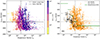 |
Fig. 2. Relationship between the measured velocity, vwind, and the final expansion factor value, fss, computed with PFSS from the back-mapping applied to the data in Fig. 1. Panel a: The wind speed, vwind, measured by Solar Orbiter as a function of the expansion factor, fss, calculated using PFSS at the source surface (located at rss). The mapping results cover from 1/08/2020 to 17/03/2022. The photospheric magnetic field is displayed with the color coding shown in the color bar, and with partial transparency to limit the masking effect. The distribution has a Pearson correlation coefficient of −0.27. Panel b: Same as panel a but colored in black for low unsigned latitudes (< 45°) and in orange for high latitude footpoints (> 45°) for each mapped observation. The typical range of values from Wang & Sheeley (1990) study, mapping observation at 1 au, are displayed by the horizontal green bars. The high and low latitudes distributions have a Pearson correlation coefficient of −0.51 and −0.24, respectively. |
Moreover, period of fast wind streams (> 500 km/s) measured by Solar Orbiter that map back to high values of fss and |Br(r⊙)| are of particular interest to the present study (top right square area). These are puzzling as they are not the common results found in the known sources of high-speed streams such as coronal holes.
Regarding magnetic field and expansion factor relation, we see that magnetic flux tubes with high fss values have strong photospheric field strengths |Br(r⊙)| (Fig. 2, panel a). This result was also reported in Wang et al. (2009) and is coherent with the fact that, during increasing solar activity, magnetic field lines with strong expansion factors tend to be rooted at low latitudes in the active region belt.
Next, we notice that the lowest |Br(r⊙)| values are only associated with vwind > 400 km/s). More globally, fss is related to |Br(r⊙)| (we checked that this is not due to the plotting point ordering, so a masking effect of earlier plotted points, by plotting |Br(r⊙)| in function of fss).
To disentangle the differences on the v–f relation between our study and the previous ones, we classified the data points according to their estimated source latitudes and split the data between high (> 45°) and low (< 45°) unsigned latitude of the source regions. The classification results are shown in panel b of Fig. 2. The plasma originating from high latitudes (black dots) follow an anti-correlation qualitatively similar as the one presented by Wang & Sheeley (1990); whereas low latitude sources do not present a specific correlation (orange dots). These classification results are supported quantitatively by the fact that the Pearson and Spearman rank correlation coefficients of the v–f distribution are −0.51 and −0.59, respectively, for the high latitude sources; only values of −0.24 and −0.26, respectively, were obtained for the low-latitude sources. This suggests that winds observed originating at low latitudes present an expansion factor value that is not intrinsically related to solar wind asymptotic speed in solar minimal activity and that other factors could come into play.
For comparison, the v–f relation obtained by Wang & Sheeley (1990) is shown as green horizontal solid bars. Some of the mapped high-latitude structures are qualitatively consistent with this v–f relation, but we must note that the two studies differ considerably in terms of the connectivity process. In fact, the relation found by Wang & Sheeley (1990) is based on daily measurements near-1 au, averaged over a three-month sliding window. The sliding average window acts as a temporal filter, removing short-duration structures. The connectivity operated by Wang & Sheeley (1990) is a direct projection of the Earth’s Carrington coordinates onto the Sun, using a default Sun-Earth transit time of 5 days. No consideration was given to magnetic field lines tracing, wind speed, or variation of the travel time. In addition, the magnetogram’s low resolution involves a spatial filtering; thus, only large-scale magnetic structures end up remaining. All these settings imply that the method of Wang & Sheeley (1990) is highlighting large-scale structures with long time duration, which match with large coronal holes characteristics. Considering a minimal solar activity, such source characteristics are typically found at high latitude.
Figure 3 is similar to panel a of Fig. 2, but colored with the measured density corrected by the radial distance r2. We observe that slow winds (< 450 km/s) are generally denser than fast winds (> 450 km/s), which is in agreement with previous solar wind studies (Schwartz & Marsch 1983; Maksimovic et al. 2020; Dakeyo et al. 2022). We also notice that fast winds with fss ≈ 100 are less dense than fast winds originating from low expansion regions. These weaker solar wind densities show that the significant magnetic field expansion is not compensated by enhancements in plasma escape from the subsonic corona.
The streamline tracing from the probe to the Sun is subject to deviation from several effects such as corotating interaction regions (CIRs) and uncertainties on the bulk speed estimation (as well as a more precise account of corotational effects). However, these effects are difficult to include in a statistical way into the mapping process. To account for their influence, we have recomputed the results of Fig. 2, applying a perturbation on ϕ(r) of ±5° and ±10° at rss. The results are presented in the Appendix A. We observe in Fig. A.2 that the overall shape presented in Fig. 2 is similar for the ±5° and ±10° panels. This indicates low variability in global trends. Consequently, this supports the existence of all the different mapped wind populations, and the reliability of the statistical mapping process itself. We refer to Appendix A for further details.
4. Expansion factor and asymptotic wind speed
The results of the back-mapping study highlight the fact that, although fast solar wind streams originating from large fss ≳ 50 regions are unexpected, as they represent a non-negligible fraction of the wind measured in the interplanetary medium.
4.1. Solar wind equations with super-expansion
We therefore considered what the physical implications of fast wind with large fss might be and how such a wind could be explained theoretically. The fast solar wind acceleration processes have been related to the fss value by Wang (1993), who introduced the idea that fss and the efficiency of the heating mechanism are anti-correlated. In fact, these authors showed that wind originating from open magnetic field lines with small fss values experiences sustained heating over a higher range of altitudes, including the region above the sonic point and inducing greater terminal speeds to be reached. In contrast, solar wind forming along field lines undergoing large expansion is heated primarily below the sonic point, thereby increasing plasma density at the expense of efficient plasma acceleration. This point of view is widely supported and used in the literature (Verdini & Velli 2007; Wang et al. 2009; Chandran et al. 2011; Pinto & Rouillard 2017; Shi et al. 2023). However, at first glance, we note that this theory does not explain how a large fss region would end up hosting high-speed streams.
Flows in a diverging flux tube can be described by the Hugoniot equation, which is more commonly used in fluid mechanics in the de Laval nozzle (Seifert et al. 1947). Extending this modeling to the solar wind leads us to the equations developed by Kopp & Holzer (1976). In their momentum expression in Eq. (6), the Mach number gradient dM/dr multiplied by the factor (M2 − 1) and the flux tube area gradient dA/dr are of same sign in the case of a subsonic flow regime (M < 1) and of opposite signs for a supersonic flow regime (M > 1). This implies that if the plasma speed of the wind is large enough low in the solar corona, a super-radial expansion can lead to an increase in the flow speed. Figure 4 of Kopp & Holzer (1976) illustrates the transition between the two types of flow regime which happens for a critical value of maximal expansion factor value fm (depending on the other model parameters). Below this limit, the flow is completely subsonic up to several r⊙ (r ≈ 4.5 r⊙ in their example); above the limit, the sonic point location jumps much closer to the Sun (r ≈ 1.3 r⊙), giving supersonic flow and large speeds in the high corona. Moreover, the larger the fm value, the more the wind is accelerated. Since the fm critical value depends on the modeled coronal condition (temperature profiles, polytropic index value), a single value representative of all the wind cases given in Fig. 2 cannot be determined.
Following the development of Kopp & Holzer (1976) applied to the isopoly hypotheses, we complete the isopoly equations including the super-radial expansion with an expansion factor profile f(r). The conservation of mass flux is re-written as follows:
 (6)
(6)
where C a constant determined from observations. The resolution of Eq. (2) including f(r) follows the same development as in Dakeyo et al. (2022), with an additional term in the derivative of the density:
![Mathematical equation: $$ \begin{aligned} \frac{d \tilde{n}_{\rm s}}{d r} = - \frac{1}{n(r_{\mathrm{iso} |\mathrm{s}})} \frac{C}{f r^2} \bigg [ \frac{2}{ur} + \frac{1}{u^2} \frac{du}{dr} + \frac{1}{uf} \frac{df}{dr} \bigg ]\cdot \end{aligned} $$](/articles/aa/full_html/2024/11/aa51272-24/aa51272-24-eq8.gif) (7)
(7)
Here,  . Its inclusion in the momentum Eq. (2) leads to:
![Mathematical equation: $$ \begin{aligned} \frac{du}{dr} \underbrace{\bigg [1-\frac{c^2}{u^2} \bigg ]}_{a(r,u)} = \underbrace{\frac{1}{u r} \bigg [c^2\bigg (1 + \frac{r}{2} \frac{d \log f}{dr} \bigg )-\frac{G M}{r}\bigg ]}_{b(r,u)}, \end{aligned} $$](/articles/aa/full_html/2024/11/aa51272-24/aa51272-24-eq10.gif) (8)
(8)
where c2 = ∑s = {p, e}cs2xs,  , and from Eq. (3) the distance, riso|s, below which the expansion is isothermal. Equation (8) is similar to the isopoly Equation (B.8) presented in Dakeyo et al. (2022), with an extra term related to f(r) expressing the effect of the super-radial expansion on the change in velocity. This extra term is positive for a flux tube monotonously expanding outward.
The starting point of the resolution is fixed at the critical radius, rc, where both a(r, u) = 0 and b(r, u) = 0. The first condition implies that this always occurs for u = c independently of the expansion profile f(r). The second condition, b(r, u) = 0, defines rc. In Dakeyo et al. (2022), rc was found to be present always in the isothermal region of the model. From Eq (8) a larger tube expansion should imply a lower rc, then rc stays in the isothermal region, and we remind xs = 1 for γs = 1. Finally, the transonic solution crosses the sonic point at rc with the condition du/dr ≠ 0. In contrast to the resolution of Eq. (2) (equivalent to the case f(r) = 1) where the sonic point is unique, solving Eq. (8) with f(r) presents possibly two distinct sonic points with only one related to a solar wind solution. The determination of the appropriate rc value is given numerically by first integrating the equation from the largest rc possible value (satisfying b(r, u) = 0), with positive u(r) derivative, in the sunward direction. If the computed solution preserves u(r < rc) < uc, it is kept. Otherwise, we redo the calculation with the other possible rc value (the smallest one), with positive u(r) derivative at rc.
4.2. Fast wind with large fss values
An example of the resolution of Eq. (8) is presented in Fig. 4, using as f(r) the widely used profile of Kopp & Holzer (1976):
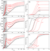 |
Fig. 4. Isopoly models with super-radial expansion described by Eq. (9). The solutions embedding subsonic and supersonic regimes below 2.5 r⊙ are displayed in black solid line and red solid lines, respectively. The left panels show isopoly solutions for the same initial parameters (Tp0 = 1.63 MK, Te0 = 0.71 MK, riso|p = 13.6 r⊙, riso|e = 10.3 r⊙, γp = 1.52, γe = 1.23), with varying expansion factor parameters (fm, re, σe), and the right panels show the associated f(r) profiles; Panel a: Different values of fm (maximum expansion factor obtained for large r); Panel b: Different values of re (radius at which the super-expansion almost stops); Panel c: Different values of σe (broadness of the expansion region). The f(r) profiles associated with panels a–c are displayed in panels d–f respectively. For all the f(r) parameters not displayed in the panel are set with (fm = 20, re = 1.9 r⊙, σe = 0.08 r⊙). While PFSS is not used here, we still mark the region located below the source surface with the gray area as a guide for comparison. |
 (9)
(9)
where the parameter f1 is selected to set fK(r⊙) = 1 as follows:
 (10)
(10)
The expansion profile, fK(r), represents a monotonously increasing super-radial expansion with r, with the main extra expansion concentrated just below r = re with a broadness σe. The expansion at large distance (r ≫ re + σe) is defined by fm.
Figure 4 extends the parametric study of the velocity profile dependence presented by Kopp & Holzer (1976) to the isopoly model, adding the influence of the other free parameters of Eq. (9). The left panels of Figure 4 shows the variation for only one of the three expansion factor parameters; fm for panel a, re for panel b and σe for panel c. Each right panel shows the expansion factor profiles associated with the curves in the corresponding left panel. This example is computed with the intermediate wind speed, for the population C (population referred from A to E for slow to fast wind respectively) of Dakeyo et al. (2022), using the same input parameters (Ts, γs, riso|s) for all curves. The input values can be found in Table 1 of Dakeyo et al. (2022) and are summarized in the caption of Fig. 4.
The value of fm sets the amplitude of the super-radial expansion as shown in panel a of Fig. 4. Its effect is similar to that of a multiplicative factor (although not directly proportional to f(r) in Eq. (9)). Since the interplanetary magnetic field is almost uniform, one can directly relate fm to the magnetic intensity Br, 0 at the base of the flux tube. The parameter re, shown in panel b, sets the radius at which the super-expansion almost stops. Considering that the super-radial expansion depends on the global magnetic equilibrium and the typical height of closed surrounding magnetic structures, re is directly related to the height of the magnetic structure being considered next to the flux tube path.
The parameter σe, displayed in panel c, sets the typical distance over which the super-radial expansion occurs, namely, the expansion region length. The super-expansion occurs typically on a distance of the order of ∼5 σe. Nevertheless, as seen in the different curves for decreasing σe values, modifying only σe, while keeping the other parameters constant, also changes the effective expansion radius. Consequently its effect is dual on the f(r) profile.
In our study, we refer to subsonic solutions below rss as “f-subsonic” and to the supersonic ones as “f-supersonic” solutions. The f-subsonic and f-supersonic solutions are shown as black and red solid lines, respectively, throughout this work.
Figure 4a shows similar results to Kopp & Holzer (1976) for isopoly solutions with a limit value of fm at which there is a change from f-subsonic to f-supersonic solutions. Increasing the super-expansion until fm = 320 allows us to gain ∼150 km/s of speed, obtaining a 550 km/s wind at 1 au. Referring to the initial 5 isopoly populations (Dakeyo et al. 2022), this leads at large distances (r ≥ 10 r⊙) to a fast solar wind similar to D population (while the thermal plasma parameters are from C population).
Varying the parameter re, Fig. 4b shows the same change of solution from f-subsonic to f-supersonic for larger re values. This indicates that the further the super-expansion occurs, the more efficient it is to accelerate the wind. While Eq. (9) sets no limit on re, in practice, it is unrealistic to set re to values larger than rss ≈ 2.5 r⊙. Since PFSS results limit the flux-tube expansion below rss (Sect. 2.4), we limit re to 2.3 r⊙. With this limit and a moderate expansion (fm = 20), Fig. 4b indicates a possible extra speed at 1 au of ∼80 km/s.
A similar transition of solution is found for the last parameter σe. Figure 4c shows that f-supersonic solutions are modeled for low σe values. As discussed above in the same section, a change in σe value modifies both the expansion length and the expansion radius; thus, we cannot determine to what extent the effective expansion length plays an important role in the f-subsonic and f-supersonic modeling in this case. Nevertheless, in practice, lower values of σe could lead to a faster wind modeled by an f-supersonic solution. The gain in velocity is comparable to the results presented for fm and re.
Combining the effects of the three parameter variations presented in Fig. 4, the case where the f-supersonic solutions provides the most acceleration is for a large global expansion (fm large), set at a large expansion radius (re large) and on a narrow radial range (small σe). This parametric study points out that for the same input parameters (Tp0, Te0, riso|p, riso|e, γp, γe), the f-supersonic solution would be able to model a faster wind speed on the order of 100 km/s larger.
Moreover, the f-subsonic and f-supersonic solutions embed different radial evolution of the speed. Indeed, the mapping results presented in Sect. 3 are based on f-subsonic solutions for all the mapped data. The f-supersonic solutions might imply alterations of the back-mapping result since the velocity profile is modified (thus, the transit time as well as the streamline local angle ϕ(r)). Based on the parametric study results (Fig. 4), the use of f-supersonic models, instead of the f-subsonic used initially, could tighten the streamline (higher velocity reached closer to the Sun), shorten the travel time, and modify the isopoly estimated coronal parameters depending on the associated f(r) profiles obtained from PFSS.
The change of the estimated isopoly coronal temperature is discussed next in Sect. 4.4. Regarding the streamline and travel time modification due to the use of f-supersonic solution, we have estimated to what extent the longitude computation at rss and the travel time are affected by comparing f-subsonic to f-supersonic backmapping computation. The details of the results are available in Appendix A.3. Finally, we estimated that the streamline deviations are small enough in comparison to the backmapping process uncertainties presented in Appendix A.2. Moreover, the travel time discrepancies do not significantly influence the magnetogram chosen to compute the magnetic topology at the wind time departure overall. Thus, accounting for f-supersonic modeling in the mapping process should not significantly affect the overall results of the study.
4.3. Solar wind f-subsonic and f-supersonic expansion deduced from magnetograms
We have shown in Sect. 4.2 that other parameters, such as the super-expansion gradient and expansion radius, influence the final wind speed (without changing the coronal temperatures). This knowledge of modeling super-expansion flow regimes can be subsequently included in the isopoly modeling used for mapping. In fact, keeping the same input parameters (Tp0, Te0, riso|p, riso|e, γp, γe) and considering the f(r) profiles obtained with PFSS, it is possible to determine whether the resolution of the isopoly leads to a f-supersonic model instead of the standard f-subsonic initially used. We might then question whether the observations related to f-supersonic isopoly solutions could contain peculiarities associated with their f(r) profile compared to f-subsonic models.
To compute the isopoly profiles of mapped data with expansion modeling, we used the f(r) profiles from the PFSS calculations for r < rss and we set f(r) = f(rss) for r > rss (the fss value depends of the field line). The isopoly parameters (Tp0, Te0, riso|p, riso|e, γp, γe) from Dakeyo et al. (2022) are interpolated using measured bulk velocity with those of the five isopoly populations. Solutions are computed with Eq. (8). The computation of either a f-subsonic or a f-supersonic solution is not an arbitrary preset and it is fully constrained by both the input parameters and f(r), respecting the solving conditions mentioned at the end of Sect. 4.1. Thus, depending on the f(r) profile, the same given input parameters may lead to two possible rc values. For these values, the f-subsonic solution is associated with the farthest critical radius, while the f-supersonic solution is associated with the closest one (as explained in Sect. 4.1).
Panel a of Fig. 5 is similar to panel a of Fig. 2, showing the v–f relationship of the mapped data, but with the data classified by the type of solutions: f-subsonic (in black) or f-supersonic (in red). The f-subsonic solutions are present for less than half of the mapped observations. Moreover, the fast solar wind is only modeled by f-supersonic solutions. This implies that the role of super-radial expansion in wind acceleration is of primary importance in modeling the asymptotic wind speed.
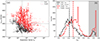 |
Fig. 5. Wind speed and typical expansion properties of the f-subsonic and f-supersonic solutions. Panel a: Same as panel a of Fig. 2 but colored (black or red) by the type of identified solutions (f-subsonic or f-supersonic, respectively) after computing isopoly models including f(r) from PFSS. The isopoly parameters are interpolated from the five populations’ isopoly parameters, from Dakeyo et al. (2022). The modeled observations include 42% and 58% of f-subsonic and f-supersonic solutions, respectively. Panel b: Typical expansion radius from Eq. (11) of the data presented in panel a classified by solution type. The f-subsonic and f-supersonic solutions are represented in black and red, respectively. |
We may now question the differences in expansion factor profiles between f-subsonic and f-supersonic solutions. To investigate this, we divided the mapped data into several fss bins and examined the shape of f(r). Considering the typical fss values related to the different existing magnetic structures, we split the data with the boundary bin values of fss = [7, 20, 50, 100, 250]. Figure B.1 presents the classified f(r) profiles. The color code is the same as panel a of Fig. 5. The median profiles are plotted in cyan solid lines and dotted lines for f-subsonic and f-supersonic, respectively. The main result is that for all the fss studied values, the f(r) profiles associated with f-supersonic isopoly solutions embed a later expansion radius than those associated with f-subsonic solutions. There is no significant difference in the expansion gradient of the f(r) median profiles between the f-subsonic and f-supersonic solutions.
To quantify the difference in expansion radius between the two types of solution, we computed a generalized typical expansion radius, rexp, similar to re, but computed for a general f(r) profile. The expansion radius is defined as the radius at which occurs the main inflection point of f(r) for an expansion increasing outward (i.e., the location of the zero of the second order derivative, while the first derivative is positive) as follows:
 (11)
(11)
In the case that f″(r) = 0 is not verified at any radius for a given profile, we assume the inflection point has not been reached yet and then we set rexp = rss.
The expansion radius distributions are shown in panel b of Fig. 5 with the same color code as in panel a. The rexp distribution of the f-supersonic solutions is shifted to a higher altitude compared to the f-subsonic one, supporting the expansion radius results of Fig. B.1. Considering that the expansion radius is related to the maximum altitude of the surrounding closed magnetic structures, the f-supersonic solutions originate from magnetic regions surrounded (on average) by higher (i.e., typically horizontally more extended) magnetic structures.
We notice that some values of rexp are identified close to rss = 2.5 r⊙ (rexp > 2.2 r⊙) and they form a small secondary distribution. This could be due to PFSS limitations implying two artifacts. First, the inflection point could be not reached below 2.5 r⊙. Second, when the associated field lines are close to the heliospheric current sheet (HCS), the source surface imposes a local divergent f(r) variation. More precisely, an artificial divergence of the field lines is implied by the source surface at the top of the closed magnetic field. This indicates that the source surface height could be too low (at best) or (more generally) that the PFSS modeling is not sufficient for these regions near the HCS. In summary, the rexp values above 2.2 r⊙ are an artifact due one of the two above limitations of PFSS modeling. However, they do not change the overall interpretation since they are relatively marginal cases. Moreover, the median values computed while excluding rexp > 2.2 r⊙ (dotted vertical lines in Fig. 5) show similar rexp separation, with an offset of ∼0.15 r⊙ between the f-subsonic and f-supersonic rexp distributions.
4.4. Updated isopoly profiles and parameters
The influence of the expansion factor on the wind models (presented in Sect. 4) reveals that if the wind populations are modeled by f-supersonic solutions, the isopoly models presented in Dakeyo et al. (2022) may embed a modification of their speed and density profile, as well as of their coronal temperature values (Tp0, Te0). Indeed, accounting for f-supersonic modeling could both decrease the required isopoly coronal temperatures and change the velocity profile in the near-Sun region (r ≤ 10 r⊙).
Moreover, it should be noted the presence of some non monotonic f(r) profiles below rss, as shown in Fig. B.1 and analyzed in Appendix B. For such profiles, f(r) first decreases, then f(r) increases with distance, which could favor wind acceleration by both subsonic and supersonic flow regimes. Indeed, a subsonic wind in the low corona in a converging flux tube receives an additional acceleration according to the de Laval nozzle effect. Next, if this wind accelerates enough to overcome the local sound speed, the wind could undergo further acceleration from the diverging part of the flux tube. The flow acceleration is then twofold, thus providing a way to model fast winds with f-supersonic solutions and a strong influence of f(r), even if f(rss) is not large.
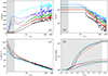 |
Fig. 6. Updated isopoly models from Eq. (8) associated with expansion factor profiles computed from PFSS, fitted to the data set used by Dakeyo et al. (2022). The f-subsonic and the f-supersonic solutions are plotted in solid and dashed lines respectively. Five isopoly models are computed for the two bins fss < 7 and 100 < fss < 250. Panel a: Updated velocity profiles; Panel b: Updated proton temperature profiles; Panel c: Updated density profiles; Panel d: Corresponding median f(r) profiles calculated from the f(r) profile obtained by the PFSS reconstruction. The data used for fitting are added in panels a–c as dots linked with straight segments. The region of super-radial expansion (up to rss = 2.5 r⊙) is delineated by the gray shaded area. The number of expansion profiles used to compute the median profiles of the [A, B, C, D, E] wind populations in panel d are [14, 16, 123, 235, 4] and [89, 360, 326, 148, 103], for fss < 7 and 100 < fss < 250, respectively. |
To take into account the above concerns, we update the isopoly speed profiles and their input parameters from Dakeyo et al. (2022) in accordance with the influence of f(r). We used the f(r) profiles computed from the PFSS algorithm presented in Fig. B.1. Since f-supersonic solutions are mostly associated with intermediate and fast winds, as seen in panel a of Fig. 5, and that these wind populations are mainly driven by protons (Dakeyo et al. 2022), we only updated the proton coronal temperatures Tp0 and left Te0 unchanged.
Given the variety of f(r) profile shapes obtained from PFSS, here we illustrate only the isopoly models for small and large super-radial expansion. To do so, we used the profiles classified by fss bins presented in Fig. B.1, and we kept the profiles in the first bin, fss < 7, and in the second to last bin, 100 < fss < 250. For each of these two fss bins, the profiles are further classified according to their measured speed, that is, we assigned each mapped observation to one of the five isopoly wind populations. This results in a total of 10 subgroups of f(r) profiles. We keep the median profiles of each subset. Consequently, for each fss bin, all isopoly populations have a unique median f(r) profile that best matches the observed speed to which they correspond. We must note that the f(r) median profiles are sensitive to the statistics used to compute each of them, so the updated isopoly profiles represent an estimate of what the speed profiles and their isopoly input parameters could be based on PFSS modeling, not a unique representation of the wind population behavior.
Figure 6 shows all the updated isopoly profiles, with the velocity in panel a, the proton temperature in panel b, the density in panel c, and the associated f(r) medians profiles in panel d. The updated isopoly parameters are presented in the Table 1, where the left value corresponds to the bin fss < 7, the right value to the bin 100 < fss < 250, and in case the parameter is unchanged it remains a single value.
The wind population A (in black) is exclusively modeled by f-subsonic solutions, and present a deceleration region between 1.5 r⊙ and 2.5 r⊙ (panel a of Fig. 6). The wind populations B and C (red and green, respectively) are associated with both f-subsonic and f-supersonic models depending on the f(r) profile selected. The f-supersonic solutions show a deceleration region above 2.5 r⊙ until ∼5 − 7 r⊙. Regarding the fast wind populations D and E (dark and light blue, respectively), they are exclusively modeled by f-supersonic solutions.
Panel b of Fig. 6 presents updated isopoly temperature profiles that are similar to the ones computed in Dakeyo et al. (2022). However, as seen in Table 1, a main difference is that Tp0 values are lower, especially for the faster winds.
Next, panel c shows that updated density profiles are significantly affected by super-radial expansion below rss in the case of f-supersonic modeling. Indeed, for the same wind asymptotic speed (red and green curves), the coronal densities are smaller with f-supersonic modeling compared to the f-subsonic one in a broad region around rss; while the effect is inverse in the low coronal region. For fast winds (blue colors), the coronal density of the f-supersonic solutions also exhibits the same behavior, with a sharp decrease between ∼1.5 and 2 r⊙. This sharp decrease induces a strong outward pressure gradient which is at the origin of the sharp wind acceleration of f-supersonic solutions. In summary, the main effect of f(r) is to modify the plasma density via the mass flux conservation. This implies enhanced pressure gradients in both the larger and more localized flux tube expansions. This implies a stronger acceleration of the wind (Figs. 4a, c and 6a). The acceleration is also stronger if the flux tube expansion is present at larger distance because the enhanced pressure gradient overcomes more easily the weaker gravity (Fig. 4c).
Finally, panel d of Fig. 6 shows that the median f(r) profiles are not as smooth as the one determined in Fig. B. They are computed on a smaller subset (of ∼5 − 350 profiles depending on the subset), which explains such weakly fluctuating shapes. However they still constitute a reliable representation of each v–f bin’s typical expansion since no strong discrepancies between them have been observed.
4.5. Implications of the updated isopoly profiles
The measurements from the interplanetary medium are closely modeled by the updated isopoly models, as shown in Fig. 6. Nevertheless, some of these updated models show relatively high-speed regions (> 250−500 km/s) below ∼7 r⊙, and a local decrease in wind speed. Thus, we may wonder how this could be consistent with remote-sensing observations of the solar corona.
In fact, several authors have observed a deceleration region in the wind radial evolution at distances below ∼7 r⊙ (Imamura et al. 2014; Bemporad 2017; Casti et al. 2023). These observations tend to support our modeling, in particular since they all focus on periods of rising solar activity, as does the present study. Moreover, they used different wind speed determination techniques. For instance Imamura et al. (2014) used radio scintillation technique, while Bemporad (2017) and Casti et al. (2023) applied the Doppler dimming technique. This observed deceleration region on such a radial interval (≲7 r⊙) could illustrate both f-subsonic and f-supersonic deceleration regions, below rss, and between rss and 7 r⊙, respectively.
The inclusion of the flux tube expansion f(r) has modified the deduced coronal temperatures as summarized in Table 1. Slow winds (A and B populations) do not see their respective proton coronal temperature Tp0 vary significantly. However, Tp0 significantly decreases for intermediate and fast winds (populations from C to E). More precisely, recalling that Tp0 = [0.65, 1.10, 1.63, 2.51, 5.61] MK with f(r) = 1 for the five wind populations studied in Dakeyo et al. (2022), the faster the wind, the more Tp0 is reduced. The temperature decrease has a maximum of 3.4 MK for the wind E, leading to an isopoly fast wind with Tp0 = 2.31 MK. The latter temperature is more in accordance to the observed one in coronal holes. This supports the assumption that the coronal temperature may decrease from the f-subsonic to the f-supersonic solution, as presented for the parametric study in Sect. 4.2.
For the simplicity of computation, the present study has only investigated modified proton parameters, while keeping electron parameters unchanged. We also recall that the isopoly parameters are not considering coronal constraints (Dakeyo et al. 2022). Consequently, to compare more realistically to coronal temperatures inferred from in situ measurements of the heavy ion charge-state ratios, our coronal isopoly temperatures should be considered an equivalent mean temperature, T0, at the base of the corona, considering T0 = (Tp0 + Te0)/2. The five isopoly mean temperatures T0 are shown on the third line of the Table 1. In particular, T0 of the fast wind (population E) can be as low as 1.6 MK, while a velocity of 620 km/s is achieved at 1 au. As a future improvement, constraining the isopoly parameters by the coronal temperature derived from remote observations and charge state measurements could be an important step to reinforce the reliability of the isopoly model and may lead to robustly constrained solar wind models.
5. Discussion and conclusions
This paper presents a statistical analysis of the speed – expansion factor relation (v–f relation), using Solar Orbiter observations and ADAPT magnetograms during minimum solar activity. For this purpose, we have established the magnetic connectivity from 01/08/2020 to 17/03/2022 when possible, using interplanetary streamline tracing and PFSS reconstruction. We assigned a solar source origin to each 30-minute average measurement. To more realistically reproduce the wind streamline trajectories from the observations, we used isopoly modeling from Dakeyo et al. (2022) to describe the radial evolution of wind properties and Weber & Davis (1967) equations to model the tangential evolution.
We find out that mixing all types of wind sources, there is only a weak global anti-correlation between the bulk speed and the expansion factor estimated at the source surface (rss = 2.5 r⊙). Consequently, studies on v–f correlation conducted on coronal holes cannot be generalized to all types of wind sources. The expansion factor on the source surface (fss) should not be the main proxy parameter for inferring the asymptotic wind speed and the radial wind acceleration profile.
We have shown the existence of a fast solar wind population originating in high magnetic field regions mainly located at low latitudes, embedding a large expansion factor and lower densities than fast winds with low fss. We explain the existence of such a wind with the generation of supersonic flows already in the low corona (below 2.5 r⊙). The coronal super-radial expansion provides an important additional source of acceleration which drives supersonic wind below 2.5 r⊙, resulting in a larger asymptotic velocity. The super-radial expansion in the supersonic regime can efficiently convert the thermal energy of the wind into kinetic energy. These type of solutions have been described as “f-supersonic” solutions, in contrast to “f-subsonic” that refers to being fully subsonic below 2.5 r⊙.
We performed a parametric study based on the expansion profile described in Kopp & Holzer (1976). We showed that the bulk speed at 1 au is monotonically increasing with larger maximum expansion value, fm, a shorter extension, σe, of the expansion region, and a larger radius, re (marking almost the end of super-expansion region). We conclude that the f-supersonic solutions require a lower coronal temperature to reach the same asymptotic speed than the f-subsonic solutions.
Next, we found the solar source associated with Solar Orbiter in situ observations. We derived the f(r) profiles from PFSS computations of the coronal magnetic field. Then, we incorporated these f(r) profiles in the isopoly modeling. We found that fast wind is almost exclusively associated with f-supersonic solutions. We computed the expansion radius rexp defined as the radius where the expansion f(r) increases the most. We observed that f-supersonic solutions have (on average) a higher rexp than f-subsonic ones, synonymous with the fact that f-supersonic wind types originate (on average) from sources surrounded by closed magnetic structures of higher altitude. This supports the importance of the expansion radius raised by our parametric study. Therefore, f-supersonic modeling and super-radial typical expansion radius, rexp, constitute viable tracks for studying the acceleration processes in the fast solar wind. The analysis of the uncertainties in the backmapping process (presented in Appendix A) confirms our conclusions, presented above.
As another outcome, we found increasingly large values for the initial bulk velocity, u0, for faster solar wind (Table 1). For faster wind, these values are in the range of 40−100 km/s. Such high velocities are coherent with the scenario of magnetic interchange reconnection at the base of the wind, as suggested by Gannouni et al. (2023), Bale et al. (2023). This is an interesting perspective for further investigation, especially with respect to quantifying the extent to which f-supersonic modeling and interchange reconnection mechanisms could work as complementary ingredients to provide an important acceleration low down in the corona. This could then help explain why the fast wind nearly reaches its terminal speed so close to the Sun.
Finally, for the slow solar wind, it is also important to take into account the f(r) profile, derived from coronal field models, since part of the slow wind comes from narrow open-field corridor located at the border of active regions (Baker et al. 2023, and references therein). In these regions, the presence of a strong closed magnetic field shapes the f(r) profile to get a strong expansion low down in the corona. Moreover, remote sensing velocity, temperature, and density measurements are available to constrain the low coronal part of the models Cranmer et al. (1999), Cranmer (2002), Imamura et al. (2014), Bemporad (2017), Casti et al. (2023). Finally, we anticipate significant future progress in modeling both slow and fast winds with the isopoly model, while taking into account the relevant coronal observational constraints.
https://gong.nso.edu/adapt/maps/gong/
Acknowledgments
This research was funded by the European Research Council ERC SLOW_SOURCE (DLV-819189) project. This research was supported by the International Space Science Institute (ISSI) in Bern, through ISSI International Team project #463 (Exploring The Solar Wind In Regions Closer Than Ever Observed Before) led by L. Harra. This work was supported by CNRS Occitanie Ouest and LESIA. D.V. is supported by STFC Consolidated Grant ST/W001004/1. This work made use of the Magnetic Connectivity Tool provided and maintained by the Solar-Terrestrial Observations and Modelling Service (STORMS). This work utilizes data produced collaboratively between AFRL/ADAPT and NSO/NISP. We recognize the collaborative and open nature of knowledge creation and dissemination, under the control of the academic community as expressed by Camille Noûs at http://www.cogitamus.fr/indexen.html. We thank the instrumental Solar Wind Analyser team (SWA) for valuable discussions. We acknowledge very valuable discussion with Miho Janvier, who has opened the problematic leading to this study.
References
- Abbo, L., Ofman, L., Antiochos, S. K., et al. 2016, Space Sci. Rev., 201, 55 [NASA ADS] [CrossRef] [Google Scholar]
- Arden, W. M., Norton, A. A., & Sun, X. 2014, J. Geophys. Res.: Space Phys., 119, 1476 [NASA ADS] [CrossRef] [Google Scholar]
- Arge, C. N., & Pizzo, V. J. 2000, J. Geophys. Res., 105, 10465 [Google Scholar]
- Arge, C. N., Henney, C. J., Hernandez, I. G., et al. 2013, AIP Conf. Ser., 1539, 11 [NASA ADS] [Google Scholar]
- Badman, S. T., Bale, S. D., Martínez Oliveros, J. C., et al. 2020, ApJS, 246, 23 [Google Scholar]
- Badman, S. T., Riley, P., Jones, S. I., et al. 2023, J. Geophys. Res.: Space Phys., 128, e2023JA031359 [NASA ADS] [CrossRef] [Google Scholar]
- Baker, D., Démoulin, P., Yardley, S. L., et al. 2023, ApJ, 950, 65 [CrossRef] [Google Scholar]
- Bale, S. D., Drake, J. F., McManus, M. D., et al. 2023, Nature, 618, 252 [NASA ADS] [CrossRef] [Google Scholar]
- Bemporad, A. 2017, ApJ, 846, 86 [Google Scholar]
- Bohlin, J. D. 1977, Sol. Phys., 51, 377 [NASA ADS] [CrossRef] [Google Scholar]
- Broussard, R. M., Sheeley, N. R., Tousey, R., & Underwood, J. H. 1978, Sol. Phys., 56, 161 [NASA ADS] [CrossRef] [Google Scholar]
- Burkholder, B. L., Otto, A., Delamere, P. A., & Borovsky, J. E. 2019, J. Geophys. Res.: Space Phys., 124, 32 [NASA ADS] [CrossRef] [Google Scholar]
- Casti, M., Arge, C. N., Bemporad, A., Pinto, R. F., & Henney, C. J. 2023, ApJ, 949, 42 [NASA ADS] [CrossRef] [Google Scholar]
- Chandran, B. D. G., Dennis, T. J., Quataert, E., & Bale, S. D. 2011, ApJ, 743, 197 [Google Scholar]
- Cranmer, S. R. 2002, Space Sci. Rev., 101, 229 [Google Scholar]
- Cranmer, S. R., Field, G. B., & Kohl, J. L. 1999, ApJ, 518, 937 [Google Scholar]
- Dakeyo, J.-B., Maksimovic, M., Démoulin, P., Halekas, J., & Stevens, M. L. 2022, ApJ, 940, 130 [NASA ADS] [CrossRef] [Google Scholar]
- Dakeyo, J.-B., Badman, S. T., Rouillard, A. P., et~al. 2024, A&A, 686, A12 [NASA ADS] [CrossRef] [EDP Sciences] [Google Scholar]
- Dorotovič, I. 1996, Sol. Phys., 167, 419 [CrossRef] [Google Scholar]
- Elliott, H. A., Henney, C. J., McComas, D. J., Smith, C. W., & Vasquez, B. J. 2012, J. Geophys. Res.: Space Phys., 117, A09102 [NASA ADS] [Google Scholar]
- Fox, N. J., Velli, M. C., Bale, S. D., et al. 2016, Space Sci. Rev., 204, 7 [Google Scholar]
- Gannouni, B., Réville, V., & Rouillard, A. P. 2023, ApJ, 958, 110 [NASA ADS] [CrossRef] [Google Scholar]
- Griton, L., Rouillard, A. P., Poirier, N., et al. 2021, ApJ, 910, 63 [CrossRef] [Google Scholar]
- Halekas, J. S., Whittlesey, P., Larson, D. E., et al. 2022, ApJ, 936, 53 [CrossRef] [Google Scholar]
- Hellinger, P., Matteini, L., Štverák, Š., Trávníček, P. M., & Marsch, E. 2011, J. Geophys. Res.: Space Phys., 116, A09105 [Google Scholar]
- Hellinger, P., Trávníček, P. M., Štverák, Š., Matteini, L., & Velli, M. 2013, J. Geophys. Res.: Space Phys., 118, 1351 [Google Scholar]
- Horbury, T. S., O’Brien, H., Carrasco Blazquez, I., et al. 2020, A&A, 642, A9 [NASA ADS] [CrossRef] [EDP Sciences] [Google Scholar]
- Imamura, T., Tokumaru, M., Isobe, H., et al. 2014, ApJ, 788, 117 [NASA ADS] [CrossRef] [Google Scholar]
- Insley, J. E., Moore, V., & Harrison, R. A. 1995, Sol. Phys., 160, 1 [NASA ADS] [CrossRef] [Google Scholar]
- Kopp, R. A., & Holzer, T. E. 1976, Sol. Phys., 49, 43 [NASA ADS] [CrossRef] [Google Scholar]
- Koukras, A., Dolla, L., & Keppens, R. 2022, SHINE 2022 Workshop, 68 [Google Scholar]
- Krieger, A. S., Timothy, A. F., & Roelof, E. C. 1973, Sol. Phys., 29, 505 [NASA ADS] [CrossRef] [Google Scholar]
- Li, H., Feng, X., & Wei, F. 2021, J. Geophys. Res.: Space Phys., 126, e28870 [NASA ADS] [Google Scholar]
- Lopez, R. E., & Freeman, J. W. 1986, J. Geophys. Res., 91, 1701 [Google Scholar]
- Macneil, A. R., Owens, M. J., Finley, A. J., & Matt, S. P. 2022, MNRAS, 509, 2390 [NASA ADS] [Google Scholar]
- Maksimovic, M., Bale, S. D., Berčič, L., et al. 2020, ApJS, 246, 62 [Google Scholar]
- Müller, D., St. Cyr, O. C., Zouganelis, I., et al. 2020, A&A, 642, A1 [Google Scholar]
- Neugebauer, M., & Snyder, C. W. 1966, J. Geophys. Res., 71, 4469 [NASA ADS] [CrossRef] [Google Scholar]
- Neugebauer, M., Forsyth, R. J., Galvin, A. B., et al. 1998, J. Geophys. Res., 103, 14587 [NASA ADS] [CrossRef] [Google Scholar]
- Nolte, J. T., & Roelof, E. C. 1973, Sol. Phys., 33, 241 [NASA ADS] [CrossRef] [Google Scholar]
- Owen, C. J., Bruno, R., Livi, S., et al. 2020, A&A, 642, A16 [EDP Sciences] [Google Scholar]
- Parker, E. N. 1958, ApJ, 128, 664 [Google Scholar]
- Pinto, R. F., & Rouillard, A. P. 2017, ApJ, 838, 89 [NASA ADS] [CrossRef] [Google Scholar]
- Pinto, R. F., Brun, A. S., & Rouillard, A. P. 2016, A&A, 592, A65 [NASA ADS] [CrossRef] [EDP Sciences] [Google Scholar]
- Poduval, B., & Zhao, X. P. 2004, J. Geophys. Res.: Space Phys., 109, A08102 [NASA ADS] [CrossRef] [Google Scholar]
- Poirier, N., Rouillard, A. P., Kouloumvakos, A., et al. 2021, Front. Astron. Space Sci., 8, 84 [NASA ADS] [CrossRef] [Google Scholar]
- Porsche, H. 1981, ESA Spec. Publ., 164, 43 [NASA ADS] [Google Scholar]
- Réville, V., & Brun, A. S. 2017, ApJ, 850, 45 [Google Scholar]
- Riley, P., & Luhmann, J. G. 2012, Sol. Phys., 277, 355 [NASA ADS] [CrossRef] [Google Scholar]
- Riley, P., Linker, J. A., Mikić, Z., et al. 2006, ApJ, 653, 1510 [Google Scholar]
- Rouillard, A. P., Plotnikov, I., Pinto, R. F., et al. 2016, ApJ, 833, 45 [NASA ADS] [CrossRef] [Google Scholar]
- Rouillard, A. P., Kouloumvakos, A., Vourlidas, A., et al. 2020, ApJS, 246, 37 [Google Scholar]
- Sanchez-Diaz, E., Rouillard, A. P., Lavraud, B., et al. 2016, J. Geophys. Res.: Space Phys., 121, 2830 [NASA ADS] [CrossRef] [Google Scholar]
- Sanchez-Diaz, E., Rouillard, A. P., Lavraud, B., Kilpua, E., & Davies, J. A. 2019, ApJ, 882, 51 [Google Scholar]
- Schatten, K. H., Wilcox, J. M., & Ness, N. F. 1969, Sol. Phys., 6, 442 [Google Scholar]
- Schwartz, S. J., & Marsch, E. 1983, J. Geophys. Res., 88, 9919 [NASA ADS] [CrossRef] [Google Scholar]
- Seifert, H. S., Mills, M. W., & Summerfield, M. 1947, Am. J. Phys., 15, 255 [NASA ADS] [CrossRef] [Google Scholar]
- Sheeley, N. R., Wang, Y. M., Hawley, S. H., et al. 1997, ApJ, 484, 472 [Google Scholar]
- Shi, C., Velli, M., Bale, S. D., et al. 2022, Phys. Plasmas, 29, 122901 [Google Scholar]
- Shi, C., Velli, M., Lionello, R., et al. 2023, ApJ, 944, 82 [NASA ADS] [CrossRef] [Google Scholar]
- Štverák, Å. T., Trávníček, P. M., & Hellinger, P. 2015, J. Geophys. Res.: Space Phys., 120, 8177 [NASA ADS] [CrossRef] [Google Scholar]
- Tóth, G., van der Holst, B., & Huang, Z. 2011, ApJ, 732, 102 [CrossRef] [Google Scholar]
- Verdini, A., & Velli, M. 2007, ApJ, 662, 669 [Google Scholar]
- Wallace, S., Arge, C. N., Viall, N., & Pihlström, Y. 2020, ApJ, 898, 78 [NASA ADS] [CrossRef] [Google Scholar]
- Wang, Y. M. 1993, ApJ, 410, L123 [CrossRef] [Google Scholar]
- Wang, Y. M., & Sheeley, N. R. 1990, ApJ, 355, 726 [NASA ADS] [CrossRef] [Google Scholar]
- Wang, Y.-M., Hawley, S. H., & Sheeley, N. R. 1996, Science, 271, 464 [NASA ADS] [CrossRef] [Google Scholar]
- Wang, Y. M., Sheeley, N. R., Walters, J. H., et al. 1998, ApJ, 498, L165 [NASA ADS] [CrossRef] [Google Scholar]
- Wang, Y. M., Ko, Y. K., & Grappin, R. 2009, ApJ, 691, 760 [NASA ADS] [CrossRef] [Google Scholar]
- Wang, Y. M., Robbrecht, E., Rouillard, A. P., Sheeley, N. R., & Thernisien, A. F. R. 2010, ApJ, 715, 39 [CrossRef] [Google Scholar]
- Weber, E. J., & Davis, L. 1967, ApJ, 148, 217 [Google Scholar]
- Yardley, S. L., Brooks, D. H., D’Amicis, R., et al. 2024, Nat. Astron., 8, 953 [NASA ADS] [CrossRef] [Google Scholar]
- Zirker, J. B. 1977, Rev. Geophys. Space Phys., 15, 257 [CrossRef] [Google Scholar]
Appendix A: Backmapping uncertainties
The magnetic backmapping process is known to be sensitive to a number of effects that affect the propagation of the wind and can alter its speed, density and temperature radial evolution (Nolte & Roelof 1973; Weber & Davis 1967; Sanchez-Diaz et al. 2016; Macneil et al. 2022; Dakeyo et al. 2024). This results in a potential deviation of the mapped longitude in streamline computation. We have taken into account the influence of acceleration and corotational effects as detailed in Sects. 2.1 and 2.2. However, other effects such as stream-stream and ICME-stream interaction are more difficult to quantify in a statistical study. The uncertainties are also dependent on the speed of the modeled stream. With all these considerations, it may not be relevant to estimate a single global uncertainty value over the entire process of the statistical study, from the location of the probe until r⊙. In order to provides uncertainties estimate related to our study, we present below different methods to estimate the reliability of the entire mapping process.
A.1. Mapping coordinates’ angular spread and source identification
The result of the magnetic connectivity process is sensitive to a coordinates displacement of a given field line at the source surface height. Indeed, a coordinates displacement at rss may results in a significant difference in footpoints location at r⊙. For this purpose, we aim to study the footpoints location variability at r⊙ depending the fieldline coordinates displacement at rss. To do this, we regroup the data points that are associated with the same source, and we study the spread of the source coordinates. This source extension is based on an angular step threshold applied on the coordinates.
The source classification method is computed as follows. The statistical backmapping study technique provides information on the time evolution of the mapped coordinates (θ⊙, ϕ⊙) at the Sun’s surface. The mapped coordinates displacement (δθ⊙, δϕ⊙) are expected to evolve approximately as the angle scanned by the probe at rss. Then, with continuous observations at a constant time cadence δt, (δθ⊙, δϕ⊙) are expected to evolve smoothly with time. However, when connectivity changes from one source to another, we expect to see a jump of the footpoints coordinates, resulting in much larger values of (δθ⊙, δϕ⊙) over the same time interval δt. This jump in angular displacement marks the source boundaries in our source identification method.
Since a source can be angularly extended both in latitude and longitude, we define the angular distance:
 (A.1)
(A.1)
equivalent to a norm of the angular displacement in both directions. We set as a threshold δθ, φ(r⊙)> 10° as source change criteria. The data that are not associated with a source observed at least during 0.5 days, are not used in the following statistics. We assume that below this duration, the source is not enough broad to infer realistic source angular extension.
The total angular spread, αs, at r⊙ is defined as the maximal angular distance covered for this given source:
 (A.2)
(A.2)
The total angular spread αss is similarly defined at rss. To analyze the change of the angular spread between r⊙ and rss, we defined the angular spreading ratio:
 (A.3)
(A.3)
For a given source, the quantity Qss is partly related to the mean expansion factor value since Qss is obtained by scanning the source extension, at both r⊙ and rss. Then, statistically, the field line centroid shift is expected to be greater (resp. smaller) for large (resp. small) fss values. Qss > 1 (resp. < 1) for a source which is more (resp. less) extended at the source surface than at the photosphere (linking the two regions by field lines).
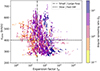 |
Fig. A.1. Relationship between the measured velocity and the expansion factor, as in Fig. 2, but colored by the angular spreading ratio Qss between r⊙ and rss as defined by Eq. (A.3). |
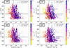 |
Fig. A.2. Effect of a systematic bias on the mapping at the source surface. The same data as in panel (a) of Fig. 2 are used but with an artificial systematic deviation of ±5° and ±10° at rss on the field line tracing. |
The results are shown in Fig. A.1. The same data points from Fig. 2 are shown except that ∼13% of the mapped data are filtered out with since they are not belonging to a source having a duration of more than 0.5 day. As expected, Qss is correlated with fss.
Moreover, considering a 1 degree angular extension at r⊙, the value of Qss is a direct measure of the angular extension at rss in degrees of the source coordinates. Consequently, the larger Qss, the less mapped coordinates (θ⊙, ϕ⊙) are sensitive to uncertainties of the mapping process, since there is a focusing effect of the field line mapping from the source surface to the photosphere. Then, sources with large Qss are localized with greater accuracy throughout the entire backmapping process (from the spacecraft to r⊙).
A.2. Unquantified streamline deviations
We estimate below to what extent streamline deviation from unquantified effects would affect our final results. Consequently we have re-computed the backmapping study and results from Sect. 3 with an artificial deviation of the longitude ϕ(rss) of ±5° and ±10°. They represent an hypothetical systematic bias. All the other parts of the magnetic connectivity process are the same as presented in Sect. 2. We observe in Fig. A.2 that the global shape presented in Fig. 2 is similar for the ±5° and ±10° panels. Some variability is mostly present for large fss values. However, this does not concern the bulk of the mapped data. We also notice that the low vwind and low fss region is less filled in the +5° and +10° maps, while it is more filled in the −5° and −10° ones.
The large vwind and large fss region is still present for all four cases with similar Br(r⊙) and fss values. Consequently, when considering relatively large variability in the mapping process, the fast wind associated with large fss regions is still observed. This statement is also supported by the fact that they typically have a large Qss (defined by Eq. (A.3)), as shown in Fig. A.1, so that the variability in streamline tracing, from the spacecraft to rss, poorly affect the location of the corresponding footpoint at r⊙.
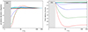 |
Fig. A.3. Streamline and travel time discrepancies between the 5 isopoly wind profiles used in the computation of the backmapping process (Dakeyo et al. 2022), and the updated 5 isopoly profiles accounting for super-radial expansion presented in Fig. 6. Panel (a): Streamline angle deviation from 1 au to rss; Panel (b): Travel time latency. The f-subsonic and the f-supersonic solutions are plotted in solid and dashed lines respectively. The wind populations, from the slowest to the fastest are shown with black, red, green, dark blue and light blue. |
A.3. Backmapping uncertainties: f-supersonic and f-subsonic deviations
The change of speed profile from f-subsonic to f-supersonic affects both the streamline calculation and the travel time, and so the mapping results. To estimate the resulting longitude deviation and time latency between f-subsonic and f-supersonic solutions, we compute the streamlines of the updated isopoly profiles presented in Fig. 6, and the travel time latency between the two types of solutions. We compare the updated streamlines and travel times with the initial ones of the isopoly profiles, used for the connectivity calculation of Dakeyo et al. (2022). This provides a post-mapping estimate of a possible supplementary error.
In order to compare the updated isopoly profiles with those of Dakeyo et al. (2022), since the asymptotic speed of each profile of the same wind population is very close to, but not exactly similar to, that of Dakeyo et al. (2022), we normalize each updated profile by the 1 au speed of its reference profile of Dakeyo et al. (2022). Regarding that the normalization coefficients are very close to 1 (≤1.08 i.e. small readjustment), we assume that it does not significantly affect the shape of the normalized profiles, which remain consistent with the non-normalized wind population speed evolution. This allows each wind population to have the same 1 au speed and set a longitude deviation from the same reference.
Panel (a) of Fig. A.3 presents the longitude deviation and panel (b) shows the time latency. These values are computed as the difference of results between the updated isopoly models and the ones computed by Dakeyo et al. (2022). The colors code is the same as in Fig. 6.
The slowest and fastest wind, populations A and E respectively, present deviations much lower than 1°. These lasts are lower than the 1° resolution of the used magnetograms, then such deviations are imperceptible in the mapping results. Next, we find a streamline deviation of about 3-4°, at rss for the wind populations B and C. Indeed, in Fig. 6, populations B and C have the largest difference of the velocity profile between f-sub and f-supersonic solutions. However, the uncertainties study presented in Appendix A.2 shows that a systematic deviation lower than 5° is not changing the overall v-f relation results.
Panel (b) of Fig. A.3 indicates that all updated f-subsonic solutions including f(r) modeling do not present any travel time latency with reference the isopoly model of Dakeyo et al. (2022). However, the f-supersonic profiles shows small to intermediate time latency, from ∼ 2 hours for fast wind and up to 5 to 8 hours for intermediate and slow solar wind. This implies that a different magnetogram should a priori be used to compute the coronal magnetic field. However, the consecutive magnetograms taken every 6 hours, do not present in general strong changes, in particular during low solar activity, as analyzed here. Moreover, this 5 to 8 hours time latency only concerns a relatively small part of the observed wind (f-supersonic solutions of winds B and C). Thus, it is expected to result in a small shift of part of the f-supersonic solutions for the B and C wind populations, but with almost no effect for other wind populations. This would introduce only small and localized changes on the v-f relation presented in Figs. 2 and 3.
Next, we notice that for the f-subsonic solutions, the modification of the speed profile exclusively takes place below rss. Then, including f(r) profile in the wind model affects neither the spiral nor the travel time. Finally, we conclude that the mapping deviation due to a change from f-subsonic to f-supersonic modeling is negligible on the statistical results presented in this article.
Appendix B: PFSS expansion factor profile
The f(r) profiles, computed with the PFSS extrapolation of magnetograms, have a broad variety of shapes. Since the results with the analytical profile of Kopp & Holzer (1976) in Sect. 4.2 show that the maximum expansion parameter is one of the key parameter, but not the only one, we divide the results into several fss bins, to study the effects of the other expansion parameters. We split the data with the fss values 7, 20, 50, 100, and 250. Figure B.1 shows all f(r) profiles separated in 6 categories. As mentioned in Sect. 4.2, for each f(r) profile an isopoly model is computed (as many models as profiles) and then assigned to f-subsonic and f-supersonic solutions. The f(r) profiles associated with f-subsonic and f-supersonic solution are plotted in black and red solid lines, respectively (as in panel (a) of Fig. 5).
A wide variety of profiles are present, although they are only partially visible due to the superposition of many cases. Then, we computed the median profiles, calculating the median value at each radial distance, of a given fss bin, between either all the f-subsonic or all the f-supersonic f(r) profiles. This allows us to derive the most typical expansion profiles, given a fss bin, and a type of isopoly solution. They are plotted in cyan solid and dotted lines for f-subsonic and f-supersonic, respectively. All these median profiles have a similar shape with a monotonous behavior. They all are nearly flat for small r values (r < 1.3 r⊙), then f(r) increases rapidly with r, to increases more steadily with r at larger r values up to rss. Then, all these monotonous profiles are mostly characterized by f(rss) and by the radius rexp with the largest slope (defined by Eq. (11)). The main difference is a larger rexp for f-supersonic solutions by about 0.2 r⊙ compared to f-subsonic ones.
Analyzing the individual profiles, some of the f(r) reconstructed from PFSS have non-monotonic profiles, with initially diverging then reconverging flux tube (visible in all panels), and the opposite case with a converging then diverging flux tube (mostly panels (a) and (b)). For example, the complexity of f(r) across a corridor of open flux is shown in Fig. 4 of Baker et al. (2023). The presence of closed fields of different magnetic flux and spatial extension around an open field region implies a differential expansion of the open flux. Some profiles have a more complex shape with possible multiple bumps of f(r) profiles. These non-monotonic profiles could be associated with closed magnetic structures surrounding the open field line, exerting a magnetic pressure that could pinch the flux tube. Several magnetic structures surrounding the same open magnetic field line may create several bumps on the flux tube expansion, and so, on the f(r) profile as well.
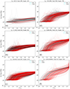 |
Fig. B.1. Expansion factor profiles, f(r), and their median profiles, based on f-subsonic and f-supersonic classification from panel (a) of Fig. 5. The f(r) profiles associated with f-subsonic and f-supersonic solutions are displayed in black and red, and their respective median f(r) profiles are plotted in cyan solid line and cyan dashed line, respectively. The number of profiles used to compute the median profiles is displayed on the top of each panel. Panels (a) to (f) correspond to fss interval with fss bins limits [7, 20, 50, 100, 250] respectively, setting six fss intervals. The larger boundary of panel (f) is set to a considerably larger value to represent infinity. |
All Tables
All Figures
|
Fig. 1. Time series of Solar Orbiter measurements from 1/08/2020 to 17/03/2022 in the period of minimal solar activity. The top panel shows the radial position of SolO. The bulk speed, vwind, proton temperature, Tp, and proton density, np, are provided by the instrument PAS, and the absolute value of the magnetic field radial component, Br, by the instrument MAG. The time intervals for which both instruments do not provide simultaneous data and the observations that are not associated with a complete backmapping process are not displayed. Each data point is a 30 minute average. |
| In the text | |
|
Fig. 2. Relationship between the measured velocity, vwind, and the final expansion factor value, fss, computed with PFSS from the back-mapping applied to the data in Fig. 1. Panel a: The wind speed, vwind, measured by Solar Orbiter as a function of the expansion factor, fss, calculated using PFSS at the source surface (located at rss). The mapping results cover from 1/08/2020 to 17/03/2022. The photospheric magnetic field is displayed with the color coding shown in the color bar, and with partial transparency to limit the masking effect. The distribution has a Pearson correlation coefficient of −0.27. Panel b: Same as panel a but colored in black for low unsigned latitudes (< 45°) and in orange for high latitude footpoints (> 45°) for each mapped observation. The typical range of values from Wang & Sheeley (1990) study, mapping observation at 1 au, are displayed by the horizontal green bars. The high and low latitudes distributions have a Pearson correlation coefficient of −0.51 and −0.24, respectively. |
| In the text | |
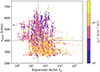 |
Fig. 3. Same as Fig. 2, but colored by measured in situ density corrected by r2. |
| In the text | |
|
Fig. 4. Isopoly models with super-radial expansion described by Eq. (9). The solutions embedding subsonic and supersonic regimes below 2.5 r⊙ are displayed in black solid line and red solid lines, respectively. The left panels show isopoly solutions for the same initial parameters (Tp0 = 1.63 MK, Te0 = 0.71 MK, riso|p = 13.6 r⊙, riso|e = 10.3 r⊙, γp = 1.52, γe = 1.23), with varying expansion factor parameters (fm, re, σe), and the right panels show the associated f(r) profiles; Panel a: Different values of fm (maximum expansion factor obtained for large r); Panel b: Different values of re (radius at which the super-expansion almost stops); Panel c: Different values of σe (broadness of the expansion region). The f(r) profiles associated with panels a–c are displayed in panels d–f respectively. For all the f(r) parameters not displayed in the panel are set with (fm = 20, re = 1.9 r⊙, σe = 0.08 r⊙). While PFSS is not used here, we still mark the region located below the source surface with the gray area as a guide for comparison. |
| In the text | |
|
Fig. 5. Wind speed and typical expansion properties of the f-subsonic and f-supersonic solutions. Panel a: Same as panel a of Fig. 2 but colored (black or red) by the type of identified solutions (f-subsonic or f-supersonic, respectively) after computing isopoly models including f(r) from PFSS. The isopoly parameters are interpolated from the five populations’ isopoly parameters, from Dakeyo et al. (2022). The modeled observations include 42% and 58% of f-subsonic and f-supersonic solutions, respectively. Panel b: Typical expansion radius from Eq. (11) of the data presented in panel a classified by solution type. The f-subsonic and f-supersonic solutions are represented in black and red, respectively. |
| In the text | |
|
Fig. 6. Updated isopoly models from Eq. (8) associated with expansion factor profiles computed from PFSS, fitted to the data set used by Dakeyo et al. (2022). The f-subsonic and the f-supersonic solutions are plotted in solid and dashed lines respectively. Five isopoly models are computed for the two bins fss < 7 and 100 < fss < 250. Panel a: Updated velocity profiles; Panel b: Updated proton temperature profiles; Panel c: Updated density profiles; Panel d: Corresponding median f(r) profiles calculated from the f(r) profile obtained by the PFSS reconstruction. The data used for fitting are added in panels a–c as dots linked with straight segments. The region of super-radial expansion (up to rss = 2.5 r⊙) is delineated by the gray shaded area. The number of expansion profiles used to compute the median profiles of the [A, B, C, D, E] wind populations in panel d are [14, 16, 123, 235, 4] and [89, 360, 326, 148, 103], for fss < 7 and 100 < fss < 250, respectively. |
| In the text | |
|
Fig. A.1. Relationship between the measured velocity and the expansion factor, as in Fig. 2, but colored by the angular spreading ratio Qss between r⊙ and rss as defined by Eq. (A.3). |
| In the text | |
|
Fig. A.2. Effect of a systematic bias on the mapping at the source surface. The same data as in panel (a) of Fig. 2 are used but with an artificial systematic deviation of ±5° and ±10° at rss on the field line tracing. |
| In the text | |
|
Fig. A.3. Streamline and travel time discrepancies between the 5 isopoly wind profiles used in the computation of the backmapping process (Dakeyo et al. 2022), and the updated 5 isopoly profiles accounting for super-radial expansion presented in Fig. 6. Panel (a): Streamline angle deviation from 1 au to rss; Panel (b): Travel time latency. The f-subsonic and the f-supersonic solutions are plotted in solid and dashed lines respectively. The wind populations, from the slowest to the fastest are shown with black, red, green, dark blue and light blue. |
| In the text | |
|
Fig. B.1. Expansion factor profiles, f(r), and their median profiles, based on f-subsonic and f-supersonic classification from panel (a) of Fig. 5. The f(r) profiles associated with f-subsonic and f-supersonic solutions are displayed in black and red, and their respective median f(r) profiles are plotted in cyan solid line and cyan dashed line, respectively. The number of profiles used to compute the median profiles is displayed on the top of each panel. Panels (a) to (f) correspond to fss interval with fss bins limits [7, 20, 50, 100, 250] respectively, setting six fss intervals. The larger boundary of panel (f) is set to a considerably larger value to represent infinity. |
| In the text | |
Current usage metrics show cumulative count of Article Views (full-text article views including HTML views, PDF and ePub downloads, according to the available data) and Abstracts Views on Vision4Press platform.
Data correspond to usage on the plateform after 2015. The current usage metrics is available 48-96 hours after online publication and is updated daily on week days.
Initial download of the metrics may take a while.