| Issue |
A&A
Volume 686, June 2024
|
|
|---|---|---|
| Article Number | A12 | |
| Number of page(s) | 8 | |
| Section | The Sun and the Heliosphere | |
| DOI | https://doi.org/10.1051/0004-6361/202348892 | |
| Published online | 24 May 2024 | |
Radial evolution of the accuracy of ballistic solar wind backmapping
1
LESIA, Observatoire de Paris, Université PSL, CNRS, Sorbonne Université, Université de Paris, 5 Place Jules Janssen, 92195 Meudon, France
2
IRAP, Observatoire Midi-Pyrénées, Université Toulouse III – Paul Sabatier, CNRS, 9 Avenue du Colonel Roche, 31400 Toulouse, France
e-mail: This email address is being protected from spambots. You need JavaScript enabled to view it.
3
Harvard-Smithsonian Center for Astrophysics, 60 Garden Street, Cambridge, MA 02138, USA
4
Mullard Space Science Laboratory, University College London, Holmbury House, Dorking RH5 6NT, UK
5
Laboratoire Cogitamus, rue Descartes, 75005 Paris, France
Received:
9
December
2023
Accepted:
1
February
2024
Abstract
Context. Solar wind backmapping is a technique employed to connect in situ measurements of heliospheric plasma structures to their origin near the Sun. The most widely used method is ballistic mapping, which neglects the effects of solar wind acceleration and corotation and instead models the solar wind as a constant radial outflow whose speed is determined by measurements in the heliosphere. This results in plasma parcel streamlines that form an Archimedean spiral (the Parker spiral) when viewed in the solar corotating frame. This simplified approach assumes that the effects of solar wind acceleration and corotation compensate for each other in the deviation of the source longitude. Most backmapping techniques so far considered magnetic connectivity from a heliocentric distance of 1 au to the Sun.
Aims. We quantify the angular deviation between different backmapping methods that depends on the location of the radial probe and on the variation in the solar wind speed with radial distance. We assess these differences depending on source longitude and solar wind propagation time.
Methods. We estimated backmapping source longitudes and travel times using (1) the ballistic approximation (constant speed), (2) a physically justified method using the empirically constrained acceleration profile Iso-poly, derived from Parker solar wind equations and also a model of solar wind tangential flows that accounts for corotational effects. We compared the differences across mapped heliocentric distances and for different asymptotic solar wind speeds.
Results. The ballistic method results in a Carrington longitude of the source with a maximum deviation of 4″ below 3 au compared to the physics-based mapping method taken as reference. However, the travel time especially for the slow solar wind could be underestimated by 1.5 days at 1 au compared to non-constant speed profile. This time latency may lead to an association of incorrect solar source regions with given in situ measurements. Neglecting corotational effects and accounting for acceleration alone causes a large systematic shift in the backmapped source longitude.
Conclusions. Incorporating both acceleration and corotational effects leads to a more physics-based representation of the plasma trajectories through the heliosphere compared to the ballistic assumption. This approach accurately assesses the travel time and provides a more realistic estimate of the longitudinal separation between a plasma parcel measured in situ and its source region. Nonetheless, it requires knowledge of the radial density and Alfvén speed profiles to compute the tangential flow. Therefore, we propose a compromise for computing the source longitude that employs the commonly used ballistic approach and the travel times computed from the derived radial acceleration speed profile. Moreover, we conclude that this approach remains valid at all radial distances we studied and is not limited to data obtained at 1 au.
Key words: Sun: evolution / Sun: heliosphere / Sun: magnetic fields / solar wind
© The Authors 2024
 Open Access article, published by EDP Sciences, under the terms of the Creative Commons Attribution License (https://creativecommons.org/licenses/by/4.0), which permits unrestricted use, distribution, and reproduction in any medium, provided the original work is properly cited.
This article is published in open access under the Subscribe to Open model. This email address is being protected from spambots. You need JavaScript enabled to view it. to support open access publication.
1. Introduction
Solar wind backmapping is a method that traces the trajectory of a solar wind plasma parcel measured in situ in the heliosphere back to its origin on the Sun (e.g., Neugebauer & Snyder 1966; Krieger et al. 1973; Burkholder et al. 2019; Rouillard et al. 2020a; Badman et al. 2020; Griton et al. 2021). Establishing this linkage is the basis of the so-called connectivity science. The solar wind connectivity typically is a two-step procedure comprising the tracing of complex magnetic field lines provided by a coronal model and a simpler treatment of the plasma trajectory above a few solar radii where the coronal field is primarily topologically open. We focus on the second part of this procedure.
In the corona, the solar wind that is emitted from its source region corotates with the Sun, and beyond a certain distance, it mostly flows in the radial direction in the inertial frame. The rotation of these sources creates a spiral pattern of wind streams from the different source regions viewed in the solar corotating frame. These trajectories can be described by the Parker spiral (Parker 1958). A given stream of plasma is frozen in to its source field line (rooted at the Sun), that is, the field line passively reflects the velocity streamlines when viewed in the corotating frame (also called the Carrington frame). Throughout this paper, plasma parcel trajectories viewed in the solar corotating frame are referred to as streamlines.
The ballistic mapping approximation estimates the streamlines of the solar wind assuming a constant radial speed measured at the location of the probe (ur(r) = uref), and zero tangential velocity (uϕ(r) = 0) everywhere. In the corotating frame, this leads to a wind streamline that follows an exact Archimedean spiral, whose azimuthal angle evolves with radius as tanϕballistic(r, uref) = r Ω⊙/uref, where Ω⊙ is the angular rotation velocity of the Sun (Snodgrass 1983). Hence, the wind stream and resulting streamline (i.e., the associated Parker spiral) becomes inclined with increasing heliocentric distance. The winding angle of the spiral is inversely proportional to the wind speed. Given an arrival time and location in the heliosphere (t, r, ϕ), the stream origin for these spiral lines at rss is easily expressed as tss = t − (r − rss)/uref and 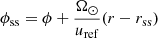 . The objective of this work is to compare (tss, ϕss) from this simple ballistic backmapping model with values derived from a more physics-based wind model that depends on the observed radial distance (r) and the solar wind speed (uref).
In more realistic models of the solar wind such as those used by Weber & Davis (1967), Nolte & Roelof (1973), Macneil et al. (2022) and Koukras et al. (2022), the plasma has a nonzero tangential speed profile. These models account for the nearly rigid corotation of the plasma near the Sun. The tangential velocity reaches a peak below the Alfvén point and subsequently decays with heliocentric distance. Recent empirical studies have identified the Alfvén point at distances between 10 and 15 R⊙, where it varies with time and different wind streams (Kasper et al. 2021; Chhiber et al. 2022; Liu et al. 2023; Badman et al. 2023). The introduction of nonzero tangential velocities leads to a straightening of the plasma streamline close to the Sun relative to the ballistic spiral and to a shift of the backmapped plasma origin to a lower longitude. However, it does not significantly affect the travel-time estimate.
The ballistic approximation can also be improved by accounting for the acceleration of the solar wind in the inner heliosphere. This aspect was accounted for by Parker (1958), and it was recently measured directly as close to the Sun as 13.3 R⊙ (Maksimovic et al. 2020; Dakeyo et al. 2022; Halekas et al. 2022). The specific acceleration profile strongly depends on the asymptotic wind speed. The acceleration of the slowest solar wind (∼350 km s−1 at 1 au) is non-negligible and extends over large heliocentric distances (by ∼100 km s−1 from 0.1 au to 1 au) (Dakeyo et al. 2022). The solar wind speed is reduced by a factor up to two-thirds at 0.1 au compared to its value at 1 au. The effects on the spiral clock angle are expected to be significant. In the absence of tangential flows, the acceleration causes the spiral to become less tightly wound closer to the Sun than in the ballistic approximation. The use of an acceleration profile affects the expected travel time because the plasma parcel spends a substantial portion of time traveling at slower speeds than its given speed uref.
With these limitations in mind, the ballistic approach is not a physically well-justified representation of the solar wind streamline. Nevertheless, Nolte & Roelof (1973) have shown that the effects of acceleration and the corotation act on the wind at 1au to a similar extent, but in the opposite sense (i.e., they displace ϕ0 in opposite directions). These two effects mainly compensate for each other, which provides support to the simpler ballistic backmapping. Ballistic backmapping therefore works better than expected and has long been known to be useful. As a result, it is widely used to estimate the origins of solar wind in situ plasma (Sanchez-Diaz et al. 2016; Rouillard & Sheeley 2011; Liu et al. 2020; de Pablos et al. 2021; Kruse et al. 2021; Badman et al. 2023). The limitation effects on ballistic backmapping from 1 au have been quantitatively estimated by Nolte & Roelof (1973), who reported a deviation in ϕss of ∼10 < SPSDOUBLEDOLLAR > °. In more recent work, these effects were supported statistically (Macneil et al. 2022), and the deviation was reported to be even lower for the fast wind stream (Koukras et al. 2022). However, these previous studies focused on backmapping from 1 au inward, whereas the weight of each effect is determined by the full radial profiles of ur and uϕ. This weighting suggests that the accuracy of the backmapping depends on the initial radial distance and the local solar wind speed that is used to initiate the mapping. The recent launches of the Parker Solar Probe (PSP) and Solar Orbiter (SolO) (Fox et al. 2016; Müller 2020) to orbits much closer than 1 au have made it even more important to account for the backmapping radial accuracy, as highlighted in the review on tools supporting ‘connectivity science’ by Rouillard et al. (2020b).
The radial evolution of the solar wind has been studied extensively since the late 1950s (Parker 1958). Numerous models have been proposed to describe the solar wind acceleration with distance. The radial evolution of the wind can be described by several analytical approaches. One of the most common approaches is the hydrodynamic fluid approach proposed by Parker (1958), which assumes that the wind is constituted of particles that evolve as a fluid. Another example are exospheric models in which the electron thermal pressure gradient is linked with an ambipolar electric potential that accelerates the solar wind (Lemaire & Scherer 1973; Maksimovic et al. 1997; Zouganelis et al. 2004). It has been shown that this description has an equivalent hydrodynamic expression according to Parker (2010). Other approaches include full magnetohydrodynamic (MHD) modeling of the solar wind, accounting for the Lorentz force, instabilities, and non-Maxwellian particle distributions (e.g., Sachdeva et al. 2019; Réville et al. 2020).
For the purpose of our work, one of the most important aspects is to model the radial evolution of the solar wind properties well. Applying radial evolution constraints has recently become easier due to the direct measurements near and inside the solar wind acceleration region made by the PSP.
Dakeyo et al. (2022) recently developed the iso-poly fluid model. He fit model profiles to statistical wind observations at heliocentric distances between 0.1 and 1 au. Derived from Parker’s equations, the iso-poly model assumes two different thermal regimes depending on radial distance (isothermal close to the Sun, representing the region where coronal heating is effective, and polytropic in the solar wind, following the empirically determined thermal behavior). This simple assumption provides significant acceleration close to the Sun (below 15 R⊙) and fits in situ spacecraft observations of the radial profiles of speed, temperature, and density beyond. This approach has the advantage of being physics driven, and it is therefore more accurate outside the range of empirical constraints than simpler analytical profiles that could be fit to the same velocity profiles (e.g., ur(r) = a × log(r)+b).
We compute uncertainty profiles of the ballistic backmapping method as a function of initial distance by comparing the ballistic source longitudes and travel times with those predicted by incorporating acceleration and corotation. In Sect. 2 we detail the modeling methods and the results of these comparisons. To model the acceleration of the wind, we use the iso-poly profiles of Dakeyo et al. (2022) defined for five wind populations from the slow to the fast solar wind (Maksimovic et al. 2020, Sect. 2.1). For the tangential flow profile, we use the iso-poly radial speed and empirically determined Alfvén speed profiles as an input in the Weber–Davis model (Weber & Davis 1967, Sect. 2.2). In Sect. 3 we analyze these results and propose a best practice for backmapping in which ballistic mapping remains the best approach for efficiently estimating source longitude, although it is essential to consider the acceleration profiles to accurately account for travel time.
2. Comparison of backmapping methods
To estimate the uncertainties of ballistic backmapping, we compared the ballistic estimation of the footpoint location and travel time for three different cases: (a) ur = uref with a constant radial speed, (b) with an accelerating solar wind speed profile, but without corotational effects ur = ur(r), uϕ = 0, and (c) with both acceleration and corotational effects: ur = ur(r), uϕ = uϕ(r). We note that the actual backmapping cannot be observed or determined, that is, none of the backmapping methods in the literature have been fully validated by observations. However, method (c) is one of the most accurate methods known to date, and we considered it as a reference in this study.
2.1. Accelerating solar wind: Parker model
We used the iso-poly fluid model from Dakeyo et al. (2022). The first-order conservation of momentum is
 (1)
(1)
where n is the density, and Ps is the pressure, and where the sum over the species s is taken over protons (p) and electrons (e). The temperature is
 (2)
(2)
where riso|s is the distance below which the expansion is isothermal, and γs is the polytropic index. For more details about the iso-poly equations and the numerical resolution, we refer to Dakeyo et al. (2022) and Shi et al. (2022).
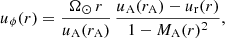
Maksimovic et al. (2020) defined five wind populations based on speed in a statistical study of Helios data. Based on these five populations, Dakeyo et al. (2022) fit the associated iso-poly modeling results. The iso-poly model solutions are presented in the left panel of Fig. 1 as solid lines. We emphasize that these models were fit to statistical datasets and therefore provide a well-constrained representation of the average speed profiles of the solar wind in the observed radial range (reaching down to 0.1 au).
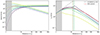 |
Fig. 1. Velocity profiles used for the comparison of the mapping methods. Left panel: radial speed profiles from the iso-poly model are shown as continuous lines (Dakeyo et al. 2022), and empirical Alfvén speed profiles are shown as dashed lines. Right panel: tangential speed profiles that account for corotation near the Sun (Macneil et al. 2022; Koukras et al. 2022). The dashed gray line represents a fully corotational solution (limit case). The pink curve represent an MHD simulation (Réville et al. 2020). The shaded gray region represents the coronal region limited upward by the source surface set at 2.5 R⊙. The dashed vertical colored lines represent the associated Alfvén radii. |
In terms of acceleration between 0.1 and 1 au, the iso-poly curves present an increase in the speed of 53%, 28%, 23%, 20%, and 17% from the slow to the fast wind. This means that the local streamline angle ϕ extrapolated at 0.1 au can involve a deviation of the same extent as the mentioned speed increase. As we show in Sect. 2.3, considering corotation without acceleration results in a substantial deviation of the mapped longitude compared to the ballistic estimate.
2.2. Corotating solar wind: Weber–Davis model
Tangential flow in the solar wind is known to be important for the purposes of ballistic mapping (Nolte & Roelof 1973; Macneil et al. 2022; Koukras et al. 2022). Based on a given radial speed profile ur(r), Weber & Davis (1967) proposed an expression for the tangential speed uϕ(r),
 (3)
(3)
where 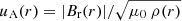 is the Alfvén speed profile, ρ(r) is the total mass density, and MA = ur(r)/uA(r) is the Alfvén Mach number.
To compute the uϕ(r) profiles, we used the five radial iso-poly speed profiles discussed in the previous section and Alfvén speed profiles uA(r). This last quantity requires a representation or model of the radial evolution of the magnetic field. Based on observations of Helios 1 and Helios 2, we estimated Br at 1 au. We used the same data set as was used by Dakeyo et al. (2022) for the magnetic field. However, due to the bimodal nature of the Br distribution (one mode per magnetic sector), it would not be representative of the typical values encountered in the solar wind to compute the average value of |B| (Badman et al. 2021). Following Badman et al. (2021), we computed an absolute average value of Br using a bi-Gaussian fit. For more details about the Br determination, we refer to Appendix A. The absolute bimodal averages are shown in Table 1, and the Br distributions are displayed in Fig. A.1. With these values and the iso-poly density profiles, we computed the associated Alfvén speed uA(r), which is plotted as dashed lines in the left panel of Fig. 1. The crossings of the dashed and solid colored curves define the associated Alfvén critical points rA. These values are annotated as dashed vertical bars in the right panel of Fig. 1.
Average magnitude of the radial magnetic field at 1 au for each of the five wind populations depending on the wind speed.
The tangential speed curves are plotted in the right panel of Fig. 1, and the rigid-rotation limit case is shown as the dotted gray line. Only the uϕ profiles in slow wind closely follow the rigid rotation limit until ∼3 R⊙ (≲350 km s−1), while the fast wind (≳550 km s−1) has already slipped to an essentially radial velocity vector at 2.5 R⊙. The tangential speed uϕ is comparable to ur in order of magnitude for the slow wind below 4 R⊙, which indicates that the corotational effect is strong for these winds. The tangential flows peak around 7–10 km s−1 between ∼10 and 17 R⊙ for slow winds and at about 2 km s−1 at 3 R⊙ for the fastest wind population (below the respective Alfvén point). The tangential speed profiles decrease asymptotically beyond this point.
In addition to the iso-poly models, we used ur(r) given by a fully isothermal 1D MHD solution of the wind (see Weber & Davis 1970; Réville et al. 2020) to calculate uϕ(r) with Eq. (3). The result is shown in Fig. 1 as the dashed red line. We applied the same initial condition as for the second-slowest iso-poly population (wind B) from Dakeyo et al. (2022). The evolution is similar for the MHD result and the equivalent iso-poly curve until ∼10 R⊙. At larger distances, the MHD solution gives a slower decrease of the tangential speed due to the greater acceleration at large distances provided by the isothermal expansion. However, the Alfvén speed and Alfvén radius are almost the same in both solutions (a relative difference of 5% and 6%, respectively). This comparison confirms that the modeling of corotational effects under the MHD and iso-poly approaches acts similarly close to the Sun (below 20 R⊙), where the nonballistic effects become stronger.
Incorporating uϕ in the calculation of the local streamline longitude ϕ based on the expression of the Parker spiral is equivalent to adding a variation in the relative angular speed between the source and the plasma (Macneil et al. 2022),
 (4)
(4)
where ϕss is the longitude location at rss, and r1 is the distance from which the backmapping is computed.
2.3. Comparison of mapping methods
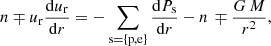
For the comparison, we assumed that a parcel of solar wind leaves the Sun in the solar equatorial plane at longitude ϕss, and we compared the trajectory of this plasma parcel with the three different methods. This was applied for the different iso-poly speed populations. The right panel of Fig. 2 shows the computed streamlines, and the left panel shows the radial evolution of the spiral longitude ϕ. The ranges of the heliocentric distances covered by Parker Solar Probe, Solar Orbiter, and Ulysses (Fox et al. 2016; Müller 2020; Wenzel et al. 1992) are indicated in the left panel. We recall that the mapping methods are referred to: ballistic (a), accelerating solar wind (b) and accelerating and corotating solar wind (c).
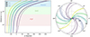 |
Fig. 2. Comparison of the mapping method streamlines. Left panel: streamline angle ϕ in the corotating frame from Eq. (4) of the five iso-poly wind populations presented in Fig. 1. Each iso-poly wind speed population is emitted from a different longitude ϕss = (0°, 30°, 50°, 65°, and 80°) from slow to fast. The streamline angle profiles are computed for the three mapping methods of a ballistic (a), accelerating solar wind (b), accelerating, and corotating solar wind (c). Right panel: Parker spirals (i.e., streamlined spiral) applied to the five iso-poly wind populations until 1 au, with the same line description as in the left panel. |
Figure 2 shows that methods (a) and (c) lead to a very similar evolution for all wind populations at all sampled distances up to 3 au, while method (b) shows an offset with (c) close to the Sun, especially for slow winds.
For method (b), the angle ϕ directly increases at the base of the streamline with r. This behavior is caused by the assumptions of neglecting corotational effects while accounting for the acceleration in the backmapping process (Nolte & Roelof 1973). The two effects no longer compensate for each other, and the slow radial velocity combined with a significant tangential drift (i.e., uϕ = 0 in the corotating frame) leads to a larger local streamline angle. The slower the wind, the larger the local streamline angles.
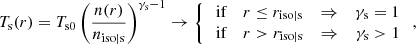
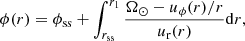
The relative angular deviations of the three methods are presented in the left panel of Fig. 3 and are summarized in Table 2 for the ranges of heliocentric distance covered by Parker Solar Probe, Solar Orbiter, and Ulysses for different latitudes. In the ecliptic plane, fast wind streamlines always show a relative deviation smaller than 1″, regardless of the distance and method. The method with the accelerating wind can deviate from the reference method (accelerating and corotating wind) by ∼6° for an intermediate wind until ∼18° for the slowest wind population over 3 au. The differences between the ballistic and the reference method for slow winds increase with distance until they reach ∼4° at 1 au, then they decrease to ∼1° for the slow wind at 3 au (647 R⊙). For intermediate and fast winds, the deviation is smaller than 2° for all distances. These results suggest that for the typical range of heliocentric distances covered by Parker Solar Probe, Solar Orbiter, and Ulysses, the ballistic mapping method provides a satisfactory estimate of the source longitude compared to reference method for a maximum deviation of 4°. The reference method is physically justified to incorporate radial acceleration wind and the corotational effect. Ballistic mapping therefore does not differ much at all studied heliocentric distances, which justifies its use within and beyond 1 au. Deviations were also computed for the meridional region (30° latitude) and the polar region (60° latitude). The meridional results are very similar to the results in the ecliptic plane, and we therefore do not display them here. The polar results show an increase in the ballistic method compared to the reference method on average.
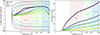 |
Fig. 3. Comparison of the mapping characteristics for all calculated methods. Left panel: relative angular deviation of the streamline from ϕss in the compared mapping methods in the longitudinal Carrington coordinates. We show the ballistic (a), accelerating solar wind (b), and the accelerating and corotating solar wind (c). Right panel: travel-time difference: Δτ profiles from Eq. (5), computed by subtracting the ballistic travel time τbal to the iso-poly travel time τip for the five wind populations. The regions of space measured by PSP, Solar Orbiter and Ulysses are colored in both panels. |
Relative streamline angular deviation Δϕ between methods (a) and (c) and between (b) and (c) for the typical range of heliocentric distances covered by PSP (0.05–0.3 au), SolO (0.3–1 au), and Ulysses (> 1 au) based on the iso-poly ur profiles.
That the corotational effect is compensated for by the acceleration through the radial acceleration profile between the Sun and the measurement point. For the only weak acceleration close to the Sun, corotational effects are not compensated for completely, and the streamline angle is deflected. Therefore, the differences between the ballistic streamline and an accelerating and corotating streamline are stronger when ur and uϕ are of similar magnitude, that is, for the slow solar wind.
We computed the travel time to estimate the plasma departure time at the source tss. This aspect of the backmapping is particularly important because the heliospheric backmapping procedure only provides an accurate location at the outer edge of the corona. To connect the solar wind to its photospheric footpoints requires coronal modeling and therefore a choice of the boundary condition of the magnetogram (Schatten et al. 1969; Levine et al. 1977). Backmapping can provide the time at which this boundary condition must be taken. This information also informs remote observers of the most relevant time to observe a given photospheric source region in order to connect it to in situ measurements (Rouillard et al. 2020a; Badman et al. 2023).
We estimated the difference between the ballistic travel time from the Sun to probe τbal and the iso-poly travel time τip. This relative time latency Δτ is expressed as
 (5)
(5)
The results of Eq. (5) are presented in the right panel of Fig. 3 and are summarized in Table 3 for different heliocentric distances. We took the ballistic speed at the distance r1 as the input for the iso-poly profile at r1. We then calculated the travel times τbal and τip from r1 to rss by integration, that is, tss − t1.
Relative travel-time latency Δτ between methods (a) and (c) for the typical range of heliocentric distances covered by PSP (0.05–0.3 au), SolO (0.3–1 au), and Ulysses(> 1 au) based on the iso-poly ur profiles.
Figure 3 shows that Δτ is ∼2–3 h for fast solar wind (∼650 km s−1 at 1 au). The persistence of source structures for the fast wind such as large coronal holes is typically a few days to weeks, and therefore, Δτ is negligible. However, for slow winds (< 350 km s−1 at 1 au), Δτ reaches 35 h at 1 au and more than 40 h near 3 au (∼1.5 days). This leaves sufficient time for the magnetic structure of the source to evolve, which might lead to a poor representation of the coronal configuration at the time of plasma release. This is emphasized by the typical source location of the slow solar wind assumed near active regions, which evolves on a faster timescale than large coronal holes. In the worst case, in situ observations of the slow wind could be associated with the wrong source.
3. Discussion
We compared the ballistic backmapping method with other methods that include the effects of solar wind acceleration and solar corotation. The backmapping method with an accelerating and corotating wind was taken as the reference method. Intuitively, backmapping models that account for acceleration and corotation are generally expected to be more physical and thus more accurate. We provided further evidence that these effects compete effectively with each other and ultimately lead to a satisfactory performance of ballistic backmapping. It results in a maximum deviation of 4° from the reference method for all explored radial distances and wind speeds. The fastest wind deviates least in the mapping at all distances. We showed that this statement also holds for backmapping that starts closer to the Sun than 1 au. Moreover, ballistic mapping always maps to a slightly larger longitude than the reference model predicts, and therefore, corotation generally has a similar but slightly weaker effect than acceleration. These results are important given the interest in connectivity science using spacecraft such as the Parker Solar Probe and Solar Orbiter in the inner heliosphere.
Backmapping deviations depend on the chosen speed profile. We calculated the profile with iso-poly modeling constrained with observed statistical data (Dakeyo et al. 2022). While other modeling choices might lead to a different detailed evolution of the deviation (Maksimovic et al. 1997; Zouganelis et al. 2004), the theoretical similarities mentioned by Parker (2010), and the one between iso-poly and MHD solution (Fig. 1) suggest that this variation will not affect the overall conclusion strongly.
However, even when an acceptable estimated location of the source in Carrington coordinates is provided (Nolte & Roelof 1973), ballistic backmapping can substantially underestimate the travel time of a given plasma parcel. Consequently, the most appropriate magnetogram for driving a coronal model relevant to backmapping may be more than a day late when it is selected on the basis of the ballistic travel time. Over this period of time, the coronal magnetic field configuration can change significantly, which might lead to potentially incorrect coronal mapping results and incorrect associations of the in situ wind characteristics with sources.
The results of backmapping method (b), which used iso-poly acceleration profiles without considering the effects of corotation, miscalculates the source longitude, but yields a more physically justified travel time. Backmapping of the fast solar wind depends only weakly on the acceleration and tangential flow profiles for the three investigated backmapping methods, and it results in smaller deviations in source longitude and travel time compared to the slow wind. For the backmapping process below 1 au, the smaller the initial radius, the smaller the deviations.
The very slow solar wind population is still accelerated at large heliospheric distances (Maksimovic et al. 2020), but the iso-poly model does not reproduce this trend at distances greater than 100 R⊙ (Dakeyo et al. 2022). This slight disagreement might result in a small deviation in the spiral angle. This effect is particularly strong in the case of the baseline solar wind (Sanchez-Diaz et al. 2016; Maksimovic et al. 2020), from which the slowest observed solar wind speeds are reported. Wind with a strong acceleration above rss deviates more strongly from the ballistic mapping regardless of the asymptotic speed.
Another limitation of our study is that we did not account for stream interactions (Sanchez-Diaz et al. 2016), which could play a role in the field line modification and travel time and might thus propagate additional deviation in the backmapping results. This also holds for the solar wind in the vicinity or behind interplanetary coronal mass ejections. These are smaller-order effects that might affect the reference method we used for the study and so the comparison results.
Based on our study, we conclude by recommending a best practice for solar wind backmapping. It is appropriate to calculate a streamline using a ballistic approximation to estimate the Carrington longitude. On the other hand, to estimate its travel time, it is more relevant to use an accelerating solar wind speed profile. These models are computationally easy, and source code for models like this can be found in Badman et al. (2023)1. Our recommendation avoids the need of full MHD simulations or a detailed knowledge of the true corotation profile for a given stream.
This study focused on the interplanetary magnetic connectivity, but a complementary study must address the field line tracing in the coronal region (i.e., below the source surface). The near Sun region is the main acceleration region for the solar wind, which means that the radial velocity is far lower (only a few dozen km s−1), so that the travel time from the surface (low corona) until rss could reach several hours and be non-negligible in the total time travel estimation.
Acknowledgments
This research was funded by the European Research Council ERC SLOW_SOURCE (DLV-819189) project. This research was supported by the International Space Science Institute (ISSI) in Bern, through ISSI International Team project #463 (Exploring The Solar Wind In Regions Closer Than Ever Observed Before) led by L. Harra. This work was supported by CNRS Occitanie Ouest and LESIA. D.V. is supported by STFC Consolidated Grant ST/W001004/1. This work made use of the Magnetic Connectivity Tool provided and maintained by the Solar-Terrestrial Observations and Modelling Service (STORMS). We recognize the collaborative and open nature of knowledge creation and dissemination, under the control of the academic community as expressed by Camille Noûs at http://www.cogitamus.fr/indexen.html.
References
- Badman, S. T. 2023, https://doi.org/10.5281/zenodo.10257870 [Google Scholar]
- Badman, S. T., Bale, S. D., Martínez Oliveros, J. C., et al. 2020, ApJS, 246, 23 [Google Scholar]
- Badman, S. T., Bale, S. D., Rouillard, A. P., et al. 2021, A&A, 650, A18 [EDP Sciences] [Google Scholar]
- Badman, S. T., Riley, P., Jones, S. I., et al. 2023, J. Geophys. Res. (Space Phys.), 128, e2023JA031359 [NASA ADS] [CrossRef] [Google Scholar]
- Burkholder, B. L., Otto, A., Delamere, P. A., & Borovsky, J. E. 2019, J. Geophys. Res. (Space Phys.), 124, 32 [NASA ADS] [CrossRef] [Google Scholar]
- Chhiber, R., Matthaeus, W. H., Usmanov, A. V., Bandyopadhyay, R., & Goldstein, M. L. 2022, MNRAS, 513, 159 [NASA ADS] [CrossRef] [Google Scholar]
- Dakeyo, J.-B., Maksimovic, M., Démoulin, P., Halekas, J., & Stevens, M. L. 2022, ApJ, 940, 130 [NASA ADS] [CrossRef] [Google Scholar]
- de Pablos, D., Long, D. M., Owen, C. J., et al. 2021, Sol. Phys., 296, 68 [NASA ADS] [CrossRef] [Google Scholar]
- Fox, N. J., Velli, M. C., Bale, S. D., et al. 2016, Space Sci. Rev., 204, 7 [Google Scholar]
- Griton, L., Rouillard, A. P., Poirier, N., et al. 2021, ApJ, 910, 63 [CrossRef] [Google Scholar]
- Halekas, J. S., Whittlesey, P., Larson, D. E., et al. 2022, ApJ, 936, 53 [CrossRef] [Google Scholar]
- Kasper, J. C., Klein, K. G., Lichko, E., et al. 2021, Phys. Rev. Lett., 127, 255101 [NASA ADS] [CrossRef] [Google Scholar]
- Koukras, A., Dolla, L., & Keppens, R. 2022, SHINE 2022 Workshop, 68 [Google Scholar]
- Krieger, A. S., Timothy, A. F., & Roelof, E. C. 1973, Sol. Phys., 29, 505 [NASA ADS] [CrossRef] [Google Scholar]
- Kruse, M., Heidrich-Meisner, V., & Wimmer-Schweingruber, R. F. 2021, A&A, 645, A83 [NASA ADS] [CrossRef] [EDP Sciences] [Google Scholar]
- Lemaire, J., & Scherer, M. 1973, Rev. Geophys. Space Phys., 11, 427 [Google Scholar]
- Levine, R. H., Altschuler, M. D., & Harvey, J. W. 1977, J. Geophys. Res., 82, 1061 [Google Scholar]
- Liu, Y. C. M., Qi, Z., Huang, J., et al. 2020, A&A, 635, A49 [NASA ADS] [CrossRef] [EDP Sciences] [Google Scholar]
- Liu, Y. D., Ran, H., Hu, H., & Bale, S. D. 2023, ApJ, 944, 116 [NASA ADS] [CrossRef] [Google Scholar]
- Macneil, A. R., Owens, M. J., Finley, A. J., & Matt, S. P. 2022, MNRAS, 509, 2390 [NASA ADS] [Google Scholar]
- Maksimovic, M., Pierrard, V., & Lemaire, J. F. 1997, A&A, 324, 725 [NASA ADS] [Google Scholar]
- Maksimovic, M., Bale, S. D., Berčič, L., et al. 2020, ApJS, 246, 62 [Google Scholar]
- Müller, D., St Cyr, O. C., Zouganelis, I., et al. 2020, A&A, 642, A1 [Google Scholar]
- Neugebauer, M., & Snyder, C. W. 1966, J. Geophys. Res., 71, 4469 [NASA ADS] [CrossRef] [Google Scholar]
- Nolte, J. T., & Roelof, E. C. 1973, Sol. Phys., 33, 241 [NASA ADS] [CrossRef] [Google Scholar]
- Parker, E. N. 1958, ApJ, 128, 664 [Google Scholar]
- Parker, E. N. 2010, in Twelfth International Solar Wind Conference, eds. M. Maksimovic, K. Issautier, N. Meyer-Vernet, M. Moncuquet, & F. Pantellini, AIP Conf. Ser., 1216,, 3 [NASA ADS] [Google Scholar]
- Réville, V., Velli, M., Panasenco, O., et al. 2020, ApJS, 246, 24 [Google Scholar]
- Rouillard, A. P., Sheeley, N. R. J., Cooper, T. J., et al. 2011, ApJ, 734, 7 [Google Scholar]
- Rouillard, A. P., Kouloumvakos, A., Vourlidas, A., et al. 2020a, ApJS, 246, 37 [Google Scholar]
- Rouillard, A. P., Pinto, R. F., Vourlidas, A., et al. 2020b, A&A, 642, A2 [NASA ADS] [CrossRef] [EDP Sciences] [Google Scholar]
- Sachdeva, N., van der Holst, B., Manchester, W. B., et al. 2019, ApJ, 887, 83 [NASA ADS] [CrossRef] [Google Scholar]
- Sanchez-Diaz, E., Rouillard, A. P., Lavraud, B., et al. 2016, J. Geophys. Res. (Space Phys.), 121, 2830 [NASA ADS] [CrossRef] [Google Scholar]
- Schatten, K. H., Wilcox, J. M., & Ness, N. F. 1969, Sol. Phys., 6, 442 [Google Scholar]
- Shi, C., Velli, M., Bale, S. D., et al. 2022, Phys. Plasmas, 29, 122901 [Google Scholar]
- Snodgrass, H. B. 1983, ApJ, 270, 288 [NASA ADS] [CrossRef] [Google Scholar]
- Weber, E. J., & Davis, L. Jr. 1970, J. Geophys. Res., 75, 2419 [NASA ADS] [CrossRef] [Google Scholar]
- Weber, E. J., & Davis, L. Jr. 1967, ApJ, 148, 217 [NASA ADS] [CrossRef] [Google Scholar]
- Wenzel, K. P., Marsden, R. G., Page, D. E., & Smith, E. J. 1992, A&AS, 92, 207 [Google Scholar]
- Zouganelis, I., Maksimovic, M., Meyer-Vernet, N., Lamy, H., & Issautier, K. 2004, ApJ, 606, 542 [Google Scholar]
Appendix A: Magnetic observation from Helios
We used the revisited dataset2 from Helios 1 and Helios 2. Observations were taken only in the period of solar activity minimum from 1974 until 1977 between 0.3 to 1 au. For each magnetic sector, we applied a bi-Gaussian fit to determine the average value depending on the magnetic field sign. Under the hypothesis that Br evolves in r−2, we corrected the data from Dakeyo et al. (2022) at all distances by r2/(1au2) for each of the five winds populations for a better statistics. The observations are presented in Figure A.1. The speed population names are the same as in Dakeyo et al. (2022) (from A to E for the slow to fast wind). The Br averaged values by magnetic sector were used to compute the global average of Table 1. Because the Br distribution is asymmetric, the absolute mean between the two sectors is normalised by the respective amplitude of each Gaussian mode in the bimodal fit. The distributions are shown in Figure A.1.
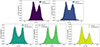 |
Fig. A.1. Distribution of the Br Helios observations at minimum solar activity, corrected by r2/(1au)2. The wind name populations are the same as in Dakeyo et al. (2022) |
All Tables
Average magnitude of the radial magnetic field at 1 au for each of the five wind populations depending on the wind speed.
Relative streamline angular deviation Δϕ between methods (a) and (c) and between (b) and (c) for the typical range of heliocentric distances covered by PSP (0.05–0.3 au), SolO (0.3–1 au), and Ulysses (> 1 au) based on the iso-poly ur profiles.
Relative travel-time latency Δτ between methods (a) and (c) for the typical range of heliocentric distances covered by PSP (0.05–0.3 au), SolO (0.3–1 au), and Ulysses(> 1 au) based on the iso-poly ur profiles.
All Figures
|
Fig. 1. Velocity profiles used for the comparison of the mapping methods. Left panel: radial speed profiles from the iso-poly model are shown as continuous lines (Dakeyo et al. 2022), and empirical Alfvén speed profiles are shown as dashed lines. Right panel: tangential speed profiles that account for corotation near the Sun (Macneil et al. 2022; Koukras et al. 2022). The dashed gray line represents a fully corotational solution (limit case). The pink curve represent an MHD simulation (Réville et al. 2020). The shaded gray region represents the coronal region limited upward by the source surface set at 2.5 R⊙. The dashed vertical colored lines represent the associated Alfvén radii. |
| In the text | |
|
Fig. 2. Comparison of the mapping method streamlines. Left panel: streamline angle ϕ in the corotating frame from Eq. (4) of the five iso-poly wind populations presented in Fig. 1. Each iso-poly wind speed population is emitted from a different longitude ϕss = (0°, 30°, 50°, 65°, and 80°) from slow to fast. The streamline angle profiles are computed for the three mapping methods of a ballistic (a), accelerating solar wind (b), accelerating, and corotating solar wind (c). Right panel: Parker spirals (i.e., streamlined spiral) applied to the five iso-poly wind populations until 1 au, with the same line description as in the left panel. |
| In the text | |
|
Fig. 3. Comparison of the mapping characteristics for all calculated methods. Left panel: relative angular deviation of the streamline from ϕss in the compared mapping methods in the longitudinal Carrington coordinates. We show the ballistic (a), accelerating solar wind (b), and the accelerating and corotating solar wind (c). Right panel: travel-time difference: Δτ profiles from Eq. (5), computed by subtracting the ballistic travel time τbal to the iso-poly travel time τip for the five wind populations. The regions of space measured by PSP, Solar Orbiter and Ulysses are colored in both panels. |
| In the text | |
|
Fig. A.1. Distribution of the Br Helios observations at minimum solar activity, corrected by r2/(1au)2. The wind name populations are the same as in Dakeyo et al. (2022) |
| In the text | |
Current usage metrics show cumulative count of Article Views (full-text article views including HTML views, PDF and ePub downloads, according to the available data) and Abstracts Views on Vision4Press platform.
Data correspond to usage on the plateform after 2015. The current usage metrics is available 48-96 hours after online publication and is updated daily on week days.
Initial download of the metrics may take a while.