| Issue |
A&A
Volume 691, November 2024
|
|
|---|---|---|
| Article Number | A362 | |
| Number of page(s) | 9 | |
| Section | Extragalactic astronomy | |
| DOI | https://doi.org/10.1051/0004-6361/202451220 | |
| Published online | 26 November 2024 | |
Reconciling concentration to virial mass relations
1
Dipartimento di Fisica e Astronomia, Alma Mater Studiorum Università di Bologna, Viale B. Pichat 6/2, 40127 Bologna, Italy
2
Instituto de Astrofísica de Canarias, Calle Vía Láctea s/n, E38205 La Laguna, Tenerife, Spain
3
Department of Physics and Astronomy, University College London, London WC1E 6BT, UK
4
Departamento de Astrofísica, Universidad de La Laguna, E38206 La Laguna, Tenerife, Spain
5
Physik-Institut, University of Zürich, Winterthurerstrasse 190, CH-8057 Zürich, Switzerland
⋆ Corresponding authors; ignacio.ferreras@iac.es, dominik.leier@gmail.com
Received:
22
June
2024
Accepted:
2
October
2024
Context. The concentration-virial mass (c-M) relation is a fundamental scaling relation within the standard cold dark matter (ΛCDM) framework well established in numerical simulations. However, observational constraints of this relation are hampered by the difficulty of characterising the properties of dark matter haloes. Recent comparisons between simulations and observations have suggested a systematic difference of the c-M relation, with higher concentrations in the latter.
Aims. In this work, we undertake detailed comparisons between simulated galaxies and observations of a sample of strong-lensing galaxies.
Methods. We explore several factors of the comparison with strong gravitational lensing constraints, including the choice of the generic dark matter density profile, the effect of radial resolution, the reconstruction limits of observed versus simulated mass profiles, and the role of the initial mass function in the derivation of the dark matter parameters. Furthermore, we show the dependence of the c-M relation on reconstruction and model errors through a detailed comparison of real and simulated gravitational lensing systems.
Results. An effective reconciliation of simulated and observed c-M relations can be achieved if one considers less strict assumptions on the dark matter profile, for example, by changing the slope of a generic NFW profile or focusing on rather extreme combinations of stellar-to-dark matter distributions. A minor effect is inherent to the applied method: fits to the NFW profile on a less well-constrained inner mass profile yield slightly higher concentrations and lower virial masses.
Key words: gravitational lensing: strong / galaxies: formation / galaxies: fundamental parameters / galaxies: halos / galaxies: stellar content
© The Authors 2024
 Open Access article, published by EDP Sciences, under the terms of the Creative Commons Attribution License (https://creativecommons.org/licenses/by/4.0), which permits unrestricted use, distribution, and reproduction in any medium, provided the original work is properly cited.
This article is published in open access under the Subscribe to Open model. Subscribe to A&A to support open access publication.
1. Introduction
The standard paradigm of galaxy formation rests on the presence of two main ingredients: dark matter and baryons. Both are subject to gravitational forces, but only the latter can be detected with photons. In this framework, dark matter represents a fundamental component, as it provides the backbone structure over large scales (cosmic web) and within the scales in which galaxies are found (haloes). The properties of dark matter haloes are thus essential to understanding galaxy formation, but these properties are limited to indirect constraints involving observations of the baryonic matter. Gravitational lensing provides a special method of detection by using the distortions exerted on the photons emitted by a background source as they pass through a gravitating structure. By ‘removing’ the contribution of the baryons from the lensing signal, it is thus possible to study dark matter haloes.
One of the main correlations found in haloes is the concentration versus mass relation (hereafter c-M, Navarro et al. 1997), by which more massive haloes tend to have progressively lower concentrations, albeit with a large scatter. This relation has been readily found in simulations (e.g. Bullock et al. 2001; Macciò et al. 2007; Dutton & Macciò 2014; Diemer & Joyce 2019; Ishiyama et al. 2021), and its scatter could unravel the details concerning the growth of haloes (e.g. Wang et al. 2020). As a first approximation, this trend is a direct consequence of the bottom-up scenario of structure formation, as lower mass haloes formed statistically at earlier cosmic times, when the density in the expanding Universe was higher (see, e.g. Mo et al. 2010). The concentration of dark matter haloes depends on the adopted cosmology (Macciò et al. 2008). However, this result is expected from a simple spherical collapse scenario, whereas a more realistic depiction would involve non-spherical structures and extended mass assembly histories, making the interpretation of concentration more complicated. Virialised haloes, in principle, should have higher concentrations (Neto et al. 2007). If the subsequent growth after the formation of the “first” structure is slow, we can expect a gradual increase of the concentration with total mass, whereas faster growth can keep the concentration unchanged (Correa et al. 2015). Therefore, variations among haloes on the c-M plane depend on their mass assembly history. The large scatter of the c-M relation found in simulations is thus an indicator of the diverse formation histories of structures. While virial mass is a good guess for a first-order parameter, more information is needed to describe the details of individual haloes (e.g. assembly bias; Wechsler et al. 2006). For instance, at a fixed halo mass, one would expect ‘older’ haloes to populate the high concentration envelope of the c-M relation. The dynamical state of a halo – shape, spin, virialisation – also affects its location on the c-M plot.
Observational constraints are harder to come by and mostly rely on the X-ray emission from the hot gas surrounding the most massive structures (e.g. Buote et al. 2007). Gravitational lensing offers a complementary method to determine the properties of dark matter haloes (e.g. Comerford & Natarajan 2007; Mandelbaum et al. 2008; Merten et al. 2015). Moreover, when restricting the lenses to galaxy scales, it is possible to constrain dark matter haloes for masses below ≲1013 M⊙ (e.g. Leier et al. 2011). However, all observational methods are based on an indirect detection of the dark matter via the gravitational potential. Simulations such as EAGLE (Schaye et al. 2015) or Illustris (Vogelsberger et al. 2014) do not suffer from this disadvantage, as the dark matter distribution is directly accessible from the simulation outputs. However, even the simulations rely on the parameterisation of mass and concentration, which require the adoption of a specific density profile function, such as those proposed by Navarro et al. (1997) or Einasto (1965).
The goal of this work is to assess the concentrations derived from strong lensing analysis over galaxy scales, which appear inconsistently high with respect to the predictions from numerical simulations (e.g. Leier et al. 2012). We show how the extracted c-M values (see Table 1) depend on resolution, modelling uncertainties, and assumptions of the underlying analytic functions, such as the dark matter profile and the initial mass function (IMF). We build upon a recent analysis of the c-M relation (Leier et al. 2022) in a sample of strong-lensing galaxies versus simulated galaxies from EAGLE using a Monte-Carlo type combination of pixelised lens models (Saha & Williams 2003) and stellar population synthesis maps, as used in Ferreras et al. (2005). In Sect. 2 we describe the data, and in Sect. 3, the method used in this study is presented.
Overview of the c − Mvir power-law parameters.
Our results in Sect. 4 show how fitted c-M relations change if the reconstructed lens profile is less well resolved in the inner part – in other words how the c-M relation changes as a function of the minimum radius. Furthermore, we demonstrate how a transformation that keeps the total enclosed mass at the Einstein radius constant but changes the steepness of the inner profile affects the c-M relation as well as the goodness-of-fit. In addition, we compare our findings with non-parametric concentrations derived from the inner radial region of lenses and simulated haloes alike. In Sect. 4.4, we show how dark matter distributions based on parametric functions other than the standard NFW profile (named after Navarro et al. 1997), change the c-M relation. Subsequently, in Sect. 4.5, we study how the adoption of different choices of the stellar IMF affects the c-M relation. Finally, in Sect. 5, we discuss whether or not all of these factors can reconcile the observed and simulated c-M relations.
2. Observed and simulated lenses
The lensing data consist of 18 systems selected to have a geometry that allows for the determination of the total mass from one to several effective radii of the lens galaxy. The sample has Hubble Space Telescope (HST) imaging in the optical (WFPC2 and ACS) and NIR (NICMOS)1, which allowed us to produce a projected stellar mass map by combining the photometry with stellar population synthesis models. This map is contrasted with a total mass map obtained from the lensing properties of the systems, adopting PixeLens (Saha & Williams 2003) as the method to solve the lensing equations. We refer the reader to Table 2 and Leier et al. (2016) for full details about the sample. We note that the derivation of stellar mass includes the possibility of a non-standard stellar IMF. We adopt two choices: the so-called bimodal IMF (BM) and a two-segment power law (2PL). More details can be found in Leier et al. (2016).
Lens data overview.
We retrieved the simulation data from EAGLE (Schaye et al. 2015), more specifically the z = 0.1 snapshot of the RefL0100N1504 run. This simulation adopts a comoving box size of 100 Mpc with 10543 dark matter particles and also includes a gas or stellar mass baryon component following standard hydrodynamical (SPH) modelling along with a set of subgrid prescriptions for the evolution of the stellar, gas, and SMBH components (Crain et al. 2015). From this sample, we selected all haloes harbouring galaxies with a stellar mass above log Ms/M⊙ = 10.75, thus representing systems comparable with the observed lenses.
As our aim is to address observed and simulated lenses with the same method, we produced projections of the mass distribution of EAGLE data in the same format as those retrieved from PIXELENS when constraining the real data. Moreover, to account for the expected variance in the haloes due to orientation, shape, and other properties, we drew an ensemble by randomly projecting the EAGLE systems (both stellar and dark matter particles) onto 100 random orientations. We then adopted the same lens geometry as the observed set – randomly assigning the parameters of one of the 18 lenses to the EAGLE data – and took the same spatial binning for full consistency. We note that we neglect the contribution of gas to the mass budget of these galaxies, a choice justified by the (high) stellar mass of the systems we targeted. In fact, the distribution of the gas to total baryon mass fraction within a projected radial distance of 15 kpc has a mean and standard deviation of 0.039 ± 0.022, justifying this approximation.
3. Lensing constraints on the c-M plane
The basic method of comparison is illustrated in Fig. 1 (applying the method to lens J0946 with the adoption of a 2PL IMF). The concentration of a dark matter halo is a manifestly difficult measurement in observations of gravitating structures. To the lowest order, one can assess the mass to light ratio (Υ ≡ M/L) through dynamical or lensing measurements within the extent of the observations. Traditionally, these constraints on Υ represent evidence of dark matter in galaxies and clusters. At the next order of reliability, one can push the data towards regions where the baryon content is negligible (usually well beyond 2.5 reff, according to Leier et al. 2011) and come up with a measurement of the total halo mass. This depends on the assumptions made to determine the extent of the halo and on the accuracy of extrapolating the observational constraints to the adopted limit of the halo. Through the use of generic models for the density profile of dark matter, one can determine a number of parameters. If the measurements extend far enough from the baryonic structure, a reliable estimate of the halo mass can be obtained. A rough approximation of the physical scales for both the luminous and total mass can be inferred from Cols. 2 and 4 of Table 2. This is also the case in simulations, where either tracing the gradient of the density profile or determining the distribution of bound particles allows one to find the limits of the halo. The standard framework of structure formation identifies total halo mass as the fundamental parameter. Indeed authors of work targeting environment-related properties in galaxies (e.g. Rogers et al. 2010; Peng et al. 2012; Pasquali 2015) have chosen halo mass as the driving factor to assess the interplay between galaxy formation and the underlying dark matter (any other dependence on halo parameters is loosely termed assembly bias).
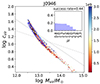 |
Fig. 1. Point cloud of successful combinations of lensing and stellar mass profiles on the c-M plane for lens J0946 representing the success rate. The colour scale indicates the MAE of the fitted models, where lower values correspond to a better goodness-of-fit. The 95% (68%) kernel density estimate contours are shown in blue (black). The solid grey line represents the c-M relation from Leier et al. (2022), while the dashed line is from Buote et al. (2007). The inset displays the frequency distribution of successful realisations as a function of the IMF slope, with very bottom-heavy IMFs leading to dark matter profiles that result in unsuccessful fits. |
The next order regarding the difficulty of derivation is the slope of the density profile. This involves a differentiation process that is much more prone to noise from variations in the distribution. To begin with, one needs to assume a radial structure (spherical, ellipsoidal, etc.), which is not necessarily a good representation in all cases, especially given the collisionless nature of dark matter particles and the long relaxation times of dark matter haloes. From this parameterisation, we derived an estimate of concentration, defined as the ratio between the virial radius (or variations thereof) and the scale radius, given by the position where the logarithmic slope is isothermal (i.e. dlog ρ/dlog r = −2). This is where the observational approach struggles. While a total mass estimate can be made without adopting many assumptions, the derivation of concentration is much more prone to the details.
In the standard methodology based on the NFW profile, the c-M relation can also be considered as a correlation between the scale radius and the virial radius. This paper focuses on how strong gravitational lensing estimates of the c-M relation can be reconciled with the theoretical expectations from numerical simulations of structure formation. In addition to the methodology described in the previous section, we include in this paper the effect of variations in the stellar IMF. The IMF is the distribution of stellar mass at birth in star forming regions. It is often treated as a universal function, based on constraints in the resolved stellar populations of the Milky Way, and usually described by either a power law (Salpeter 1955) or variations that include a tapered low-mass end and differing slopes at the massive end (see, e.g. Kroupa 2001; Chabrier 2003). Over the past decade or so, evidence has shown that the IMF can depart significantly from the canonical one, especially in the dense central regions of early type galaxies (see, e.g. Martín-Navarro et al. 2015; La Barbera et al. 2019).
In our analysis, the effect of a non-universal IMF has to do with the derivation of the stellar mass profile and hence the dark matter halo – produced as the remainder from the lensing mass distribution. In gravitational lensing systems, the IMF has proven controversial (see, e.g., Smith et al. 2015, 2017; Leier et al. 2016), showing results at odds with the alternative constraints based on stellar population analysis (e.g. van Dokkum & Conroy 2010; Ferreras et al. 2013; La Barbera et al. 2019) or dynamics (e.g. Cappellari et al. 2012; Lasker et al. 2013; Lyubenova et al. 2016). In this paper, we only consider the effect that a non-universal IMF might have in a systematic variation on the c-M plane determined for strong lenses.
4. Resolution and non-parametric concentrations
The focus of this paper is to explore in more detail the offset found in Leier et al. (2022) between observed galaxies (via gravitational lensing) and simulated galaxies. While both samples show the characteristic negative correlation between concentration and halo mass, the lensed galaxies suggest higher values at a fixed mass with respect to the simulations. Needless to say, the derivation of halo parameters from the observations is dependent on a number of assumptions, which we study in the following, that could affect the systematic bias in the comparison made on the concentration versus mass relation plane.
4.1. Inner profile
Figure 2 addresses the potential impact of the spatial resolution of the central region of the lens on the c-M relation. The results for the lens J0946 are shown (from top to bottom) when zero to three inner radial points are neglected in the fitting procedure, as labelled. The amount of available radial points is derived from a 31 × 31 grid used in the lens reconstruction method, corresponding to a resolution limit of one-fifteenth of the lens reconstruction radius, as listed in Col. 3 of Table 2. By excluding up to three inner radial points from the fit, we assessed both the influence of assuming an NFW profile on the c-M relation and the robustness of the procedure. We present the results for the two choices of stellar IMF: two power law (left column) and bimodal (right column).
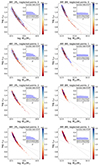 |
Fig. 2. Same as in Fig. 1 but with a lower limit added to the radial profile. The left (right) column shows the data for a two power law (bimodal) IMF. From top to bottom, we show the effect of decreasing resolution of the inner radial region by dropping the inner zero to three supporting points of the reconstructed mass profiles used for the NFW-fit. The colour bar indicates the mean average error of the fits in units of 109 M⊙. |
For all lenses as well as the given example of the lens J0946, the inner part of the mass profile has only a small impact on the cloud of acceptable fits:
-
The goodness-of-fit is improved, meaning that both the root mean square deviation (RMSD) and mean absolute error (MAE) become smaller as a consequence of the reduced number of supporting points.
-
The scatter towards low concentration and high virial mass is slightly reduced, and the distribution of points in the c-M plane becomes more concentrated
-
There are, however, no significant changes in the success rate of the fitting procedure nor any significant overall trends in the c-M distribution.
We note that the goodness-of-fit and the success rate of the fit are distinct metrics. The success rate refers to the fraction of valid stellar and lens mass combinations that satisfy the convergence criteria of the least-squares fitting routine. These criteria are not met, for instance, when a given combination of total mass and stellar mass profile yields an enclosed mass profile that is non-monotonic or decreases with increasing radius, as enclosed mass profiles must be monotonically increasing. In contrast, the goodness-of-fit is quantified by measures such as the MAE or other deviations between the model and observed data. We conclude that a well constrained mass profile extending to small radii ensures a determination of the c-M parameters with small uncertainties. Indeed we find for certain systems (especially J2347, J2303, J1531) – the ones that are less well constrained by lensing – that the concentration increases systematically with the number of neglected points. Others (e.g. J0959, J1525) show a less pronounced tendency and overlapping as well as widespread density distributions, which do not permit one to arrive at an unequivocal conclusion.
Furthermore, in cases with a clear trend between the number of neglected points and their location on the c-M plane, the effect is independent of the assumed IMF. We find that the frequency distribution of the free parameter μ of the two power-law IMFs (inset plots, Fig. 2) changes only marginally with the number of neglected points. The same applies to the free parameter Γ of the bimodal IMFs. There is only a slight tendency for both parameters to change towards higher values with an increased number of neglected points, in the sense that we lose a fraction of the μ = 0.8 points and gain a bit at μ = 1.8 − 2.0.
Hence we conclude that for a few less well-constrained lenses, the adopted mass reconstruction method may introduce a certain bias in the distribution of accepted points on the c-M plane. One way to mitigate or to avoid this issue altogether is by filtering these points with respect to the goodness-of-fit. The reconstruction method may fit the data by putting too much mass at the center of galaxies, hence altering the outcome of the fits. In some cases, however, it seems that removing a possibly biased innermost point leads to even higher concentrations. A plausible explanation for this behaviour is related to the sensitivity of the NFW-fit method to the transition within the dark matter profile from an initial power law of r−3 to the subsequent r−1.
When encountering a reconstructed enclosed mass profile that can be successfully accommodated by a singular power law, the positioning of the scale radius during the fit tends to converge toward small radii (i.e. the outermost reconstruction radius). This yields diminished values for rs and consequently results in elevated concentration values.
As a better understanding of the systematics of lens mass reconstruction and analytic fits is obtained, it seems worthwhile to investigate in detail how the output (i.e. the c-M point cloud) is affected and potentially biased by changes to the steepness of enclosed mass profiles. We focused especially on transformations that keep the enclosed mass constant.
4.2. Enclosed mass profile
Another possible bias in the derivation of the c-M relation is introduced by the radial mass profile. Gravitational lensing data feature a well-known butterfly-shaped pattern in the radial enclosed mass profile, where the uncertainties are smallest at the radial position Rlens of the lensed images (see, e.g., Fig. 1 in Ferreras et al. 2010). To quantify the effect of systematics in the derivation of the cumulative mass profile, we applied a distortion function that alters the steepness of M(< R) inside R < Rlens while preserving M(< Rlens).
For a halo taken from the EAGLE simulation, we introduced variance in the enclosed mass profile to mimic the behaviour of lens reconstruction models being less well constrained. This certainly applies to a radial region inside the lens radius. The process involves differentiating the enclosed mass profiles, namely by calculating the difference between a supporting point n and its inner neighbour n − 1 and applying the factor given by the following equation:

with the logit function defined as
followed by cumulating the profile. The parameter L in Eq. (1) defines the degree of distortion of the non-cumulative profile as shown in Fig. 3 for L = 0.1, where the inner part of the mass profile is modified to start at a value 10% lower than the original mass, and the outer part is defined to end up with a mass 10% higher than the original result. By allowing this amount of variance for EAGLE haloes, we recreated the uncertainty of the ensemble of lens models. As a result, the cloud of c-M values from acceptable NFW-fits changes from a tightly constrained region in the c-M plane to a scattered pattern, elongated along the direction of higher concentration towards lower mass haloes and lower concentration in higher mass haloes. This elongated distribution of c-M values has been found among the observed lenses if the ensemble profiles are less well constrained. They are also found in given simulated EAGLE haloes when the range of projection angles yield very different 2D maps (e.g. due to strong triaxiality). We note that independent of L, the median c and median M values are close to the real (undistorted) quantities and the density contours overlap to some degree.
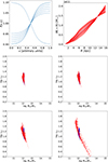 |
Fig. 3. Top left: Distortion function according to Eq. (1). The solid line represents the L = 0.1 case; the dashed lines show the cases of L = 0.09 to L = −0.1. Top right: One hundred realisations of an enclosed DM mass profile (from J1525) modified by random distortion functions with L varying from –0.5 to 0.5. Middle left to bottom right panel: Changing concentration to virial mass relation for 1000 realisation with randomly chosen L-values (0.05, middle left; 0.1 middle right; 0.2, bottom left; 0.5, bottom right) shown in red. The blue point cloud represents the fits to the original DM profiles. |
We conclude from this experiment that despite its uncertainties, the median values of the c-M fits deduced by our method should be reliable estimates of the real quantities, given that no other bias affects our lens sample. In the next section, we investigate fitting systematics affecting the parametric concentration by deriving a non-parametric concentration that is unaffected by the underlying assumption of NFW-distributed dark matter.
4.3. Parametric concentration
Since cvir is defined as the virial radius divided by the NFW scale radius, the definition strongly relies on the profiles at small radii. Therefore, it seems prudent to contrast these results with an alternative, more robust non-parametric concentration defined as R90/R50, where RX is defined as the projected 2D radius within which the mass enclosed is X percent of the enclosed total mass within two effective radii M(< 2reff). For instance, in Leier et al. (2011) it was found that the R90/R50 ratio behaved differently for the lensing and stellar mass distributions, with the stellar component being more concentrated in more massive galaxies. In our case, we wanted to assess whether R90/R50 for the total mass is also found to be different in observed and simulated galaxies. This ratio was measured directly from the lens and EAGLE ensembles and independently of the parametric fits.
In Fig. 4 we show the non-parametric concentrations (R90/R50) of the EAGLE (squares) and lens sample (circles) and compare it to the parametric concentration cvir. We highlight the goodness-of-fit in terms of median residuals of the NFW-fit by colour. The lens sample exhibits negative residuals, as the fits are larger than the data points, especially at small radii. The EAGLE sample provides small positive residuals. Although the point clouds overlap slightly, a two-sample Kolmogorov-Smirnov (KS) test for cvir and R90/R50 for a significance level of α = 0.001 rejects the null hypothesis. The two samples are thus drawn from different distributions, meaning that both the parametric and the non-parametric concentration are distinct when comparing simulated haloes and lenses. The qualitative results are not affected by excluding singular lenses nor by adding random noise. However, the error bars are not taken into account for the KS test. Considering the large uncertainties, this conclusion might be premature (especially in the presence of bias).
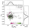 |
Fig. 4. Virial concentration versus non-parametric R90/R50. The colours represent median values of the residuals of the NFW-fits. The lens sample (circles) shows mostly large negative residuals (magenta), whereas the EAGLE sample (squares) shows small positive residuals (green). The X- and Y-axis histograms show two populations: kernel densities for the EAGLE sample (solid black line) and the lens sample (dashed grey line). A two-sample KS test for cvir and R90/R50 for a significance level of α = 0.001 indicated that the two samples are drawn from different populations. |
When we investigated the residuals of the NFW-fits, we found that most lenses exhibit strong negative residuals. In other words, the model fits yield a smaller mass than the original data – which is mostly due to departures from the NFW profile at small radii. The EAGLE haloes in contrast can be well fitted by NFW profiles with only small positive residuals.
As lens and EAGLE concentrations are distinct, according to both their parametric and non-parametric definitions, the NFW-fit itself cannot be the root cause of the c-M discrepancy. The fact that lenses are less well described by NFW profiles may however originate from the models being too concentrated in the inner radial region, as a consequence of the subtraction of baryon mass or possibility due to a known tendency of PixeLens models to oversample highly concentrated models (Lubini & Coles 2012). However, as we used the NFW-fit exactly for the purpose of getting rid of this shortcoming, we conclude that our method produces the expected results and is less affected by the reconstruction bias. After establishing that the NFW profile assumption plays a crucial role in our method (i.e. removing the aforementioned bias), we wanted to study what happens if we choose different analytic descriptions for the dark matter component.
4.4. Beyond NFW profiles
Since c-M studies are mostly based on the NFW scale radius definition of rs and hence cvir, which we are trying to reconcile with our findings, assuming different dark matter profiles may seem to be a futile exercise. However, one way of finding out whether or not an NFW profile is a well-suited representation of the ΔM(< R) = Mlens(< R)−Mstel(< R) is by checking different profile fits, the amount of feasible fits to combinations of Mlens(< R) and Mstel(< R), and their goodness-of-fit.
In this section, we change the description of the underlying analytic function, which in turn changes the significance of the scale radius used in the definition of the concentration rvir/rs. For this, we used the projected cuspy NFW profiles as defined in Keeton (2001). This model is a generalised version of the NFW profile, with a density profile of
The cumulative projected mass profiles for γGNFW = {0, 1, 1.5, 2} are as follows:
![$$ \begin{aligned} \gamma _{\rm GNFW}& = 0: M \sim 2\kappa _s r_s \times \left[ 2 \ln \frac{x}{2} + \frac{x^2 + (2-3x^2) \mathcal{F} (x)}{1-x^2} \right] \end{aligned} $$](/articles/aa/full_html/2024/11/aa51220-24/aa51220-24-eq45.gif)
![$$ \begin{aligned} \gamma _{\rm GNFW}& = 1: M \sim 4\kappa _s r_s \times \left[ \ln \frac{x}{2} + \mathcal{F} (x) \right] \end{aligned} $$](/articles/aa/full_html/2024/11/aa51220-24/aa51220-24-eq46.gif)
![$$ \begin{aligned} \gamma _{\rm GNFW}& = 1.5: M \sim 4\kappa _s r_s x^{3/2} \times \nonumber \\&\qquad \left[ \frac{2}{3} _2F_1[1.5,1.5,2.5,-x] + \right. \nonumber \\&\qquad \left. \int _0^1 dy (y+x)^{3/2} \frac{1 - \sqrt{1-y^2} }{y} \right]\end{aligned} $$](/articles/aa/full_html/2024/11/aa51220-24/aa51220-24-eq47.gif)
![$$ \begin{aligned} \gamma _{\rm GNFW}& = 2: M \sim 4\kappa _s r_s x \times \left[ \frac{\pi }{2} + \frac{1}{x} \ln \frac{x}{2} + \frac{1-x^2}{x} \mathcal{F} (x) \right], \end{aligned} $$](/articles/aa/full_html/2024/11/aa51220-24/aa51220-24-eq48.gif)
where x = r/rs, 2F1 is the hypergeometric function and
We note that we adopted the convention in which the cusp slope has positive values. We proceeded to use the extreme values presented above of γGNFW to study the impact of a non-standard mass profile on the c-M relation. This is despite the fact that only extreme concentrations allow lens systems with slopes of 0.5 that can produce multiple images (see, e.g., Mutka & Mähönen 2006) and that our sample of observed lenses exhibit quad configurations that all have very visible lensed images, which already sets boundaries for the mass distribution. By imposing different slopes in the fit, we essentially changed the impact that data at small radii have on extrapolated quantities, including the virial radius, and we also changed the meaning of the scale radius. To determine the virial radius, we considered the mass enclosed within a sphere of the profiles presented above. For the different values of γGNFW, we obtained the following enclosed masses:
![$$ \begin{aligned} \gamma _{\rm GNFW}&= 1.5: 4 \pi \rho _s r_s^3 \frac{2}{3} x^{3/2} _2F_1[1.5,1.5,2.5,-x] \end{aligned} $$](/articles/aa/full_html/2024/11/aa51220-24/aa51220-24-eq52.gif)

where x = r/rs In Fig. 5, we show the impact on concentration cvir = rs/rvir and virial mass Mvir of changing γGNFW. We restricted the plot to four out of 18 lenses, namely J0037, J0044, J0946, and J2343. The concentrations of the 10 000 random combinations of total and stellar mass (i.e. ΔM = Mtot − Ms) exhibit a trend towards lower concentration with increasing γGNFW (i.e. towards cuspier models). Beyond 0.6% of rvmax , there is a general consensus that haloes are denser than those derived from an NFW profile and that they are well fitted by functions that are steeper and cuspier than NFW at these radii, as with the GNFW profile with γGNFW = 1.2 or the Einasto profile with γ = 0.17 (e.g. Moore & Diemand 2010). While low γGNFW profiles show a turnover, which can also be seen in the lens profiles, high γGNFW profiles lack this additional constraint. Especially profiles with γGNFW = 2, which is a single power law without turnover, the fitted scale radius automatically goes to large values, and cvir consequently drops to almost zero. Profiles with γGNFW = 1.5 seem to bridge the γGNFW = 1 and 2 cases with a large scatter. As concentration and virial mass are inversely related and belong to a one-parameter family (a result from assuming one of the above dark matter functions), an increasing trend of Mvir with γGNFW follows naturally.
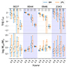 |
Fig. 5. Box plot of concentrations (top panel) and virial masses (bottom panel) plotted against γGNFW for the four lenses J0037, J0044, J0946, and J2343. Mean values and standard errors are shown as black dots with error bars in addition to the box plots showing the interquartile range (25–75%) and whiskers at the 90% confidence interval. The small vertical numbers show how many of the original 10 000 realisations produced viable fits. |
Changing the IMF does not qualitatively alter this result. However, with only a few exceptions, bimodal IMFs produce a smaller variance, as shown in Fig. 5. As can be seen for J0946, the values move gradually from non-physically large concentrations of log c > 1.5 and virial masses of 1012.5 M⊙ for γGNFW = 0 to implausibly small concentrations of log c < −1 and virial masses at around 1013.2 M⊙. The residual mean standard deviation of the fits shifts only marginally to larger values. It should be noted that small virial concentrations with γGNFW = 2 are a result of the scale radius remaining unconstrained by the adopted mass profile. For all other profiles the turnover between two different density slopes are a function of rs. Consequently, the scale radius drifts gradually towards higher values in the fitting process.
Using the scale radii of respective GNFW profiles to compute cvir shows that γGNFW = 0 and 1 profiles produce similar results in terms of goodness-of-fit (RMSD and MAE) while reducing its absolute value. The choice of GNFW also does not exclude certain combinations of Mlens and Mstel, as seen by the number of realisations producing a valid fit at the top of Fig. 5. While a smaller γGNFW produces a larger concentration, a larger γGNFW reduces the concentration. We find, however, no evidence that an NFW is a worse representation of the dark matter profiles that we produced with our method, but we acknowledge the fact that γGNFW < 1.5 profiles produce suitable fits and that by extension a real γGNFW = 0 profile falsely fitted by an NFW profile might bias the c-M results. In the next section we focus on the impact of the IMF choice on concentration and virial mass in more detail.
4.5. Stellar initial mass function
In Fig. 6 we show how the c-M parameters change for an NFW fit to the dark matter component if we assume different slopes ΓBM for the bimodal IMF defined in Vazdekis et al. (2003) and μ2PL for the two-segment power-law IMF of Eq. (13), where 𝒩 is a normalisation factor and μ is a free parameter that controls the fractional contribution in low-mass stars.
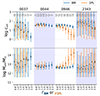 |
Fig. 6. Parameters of c-M as a function of IMF slopes ΓBM for a bimodal IMF (blue) and μ2PL for a two-segment power-law IMF (orange) in case of an NFW γ = 1 fit to the residual enclosed mass profiles. The box plots show the interquartile range plus 90% CI as whiskers. The black dots and error bars show the mean values with standard errors. |
We note that for the bimodal case, Γ > 1.3 represents a more bottom-heavy IMF than Kroupa (2001), whereas for the two-segment power-law function, μ > 1.3 is more bottom-heavy than Salpeter (1955). For the two-segment power law, a substantial drop in concentration and an increase in virial mass can be observed beyond μ = 1.5. Although less pronounced, this trend can be confirmed for the bimodal IMF, too. We note that for J0037 and J0044, the bottom-heavy end of the two-segment power law could be ruled out, as none of the stellar mass maps produced enclosed masses smaller than their respective total mass. The property to constrain the range of the IMF slope was studied in Leier et al. (2011) and can be seen in the inset histogram of Fig. 1.
Through Figs. 7 to 9, we reconfirm the results from the previous section and show the systematic impact of the IMF slope on the c-M relation. Significant differences in the distributions of c and M are visible only if we go to extreme choices for ΓBM and μ2PL, respectively. Only more well-constrained lensing systems, such as J0946, are capable of showing the trend with sufficient significance.
5. Discussion
In this paper, we present a series of findings regarding a number of factors that may influence the conclusions in Leier et al. (2022) concerning the offset on the concentration-mass plane of observed and simulated dark matter haloes. In particular, we show the following:
-
Via strong lensing, we probed the inner radial region up to the scale radius of the targeted DM profiles. The adoption of cuspier profiles that can produce slightly better fits causes the scale radius to increase faster than the extrapolated virial radius, effectively leading to lower estimates of concentration. The case of γ ∼ 2 yields a single power-law distribution without discernible turnover and scale radius, causing the fits to reach extreme values and hence producing unrealistically low concentrations. Nevertheless, we noticed a significant negative (positive) trend between c (M) and γGNFW when going from γGNFW = 0.5 to 1.5. The uncertainties vary strongly among the lenses in our sample. However, changes of ∼0.3 dex in log c with every 0.5 step in γGNFW can be explained.
-
The fact that in some cases GNFW produces better fits suggests a strong impact of the inner radial region, which should be considered as well when interpreting the results of the NFW fits. Moreover, this suggests that the substructure – which also introduces a departure from an NFW profile – may also induce a higher concentration. The inherent limitations of the simulation data lead to better NFW fits and thus a lower concentration.
-
Furthermore, we find that changes to the lens mass profile affecting its steepness for r < rEin cause more widespread distributions in the c-M plane in terms of both concentration and virial mass. This explains the lens-to-lens variation in terms of the quality of the available constraints. Less well constrained lenses permit a wider range of slopes. Shallower profiles at low radius produce lower concentrations but higher virial masses and vice versa.
-
By introducing a non-parametric concentration based on the curve of growth, R90/R50, we find tentative evidence that the differences in the concentration to virial mass plane presented in Leier et al. (2022) can be traced back to differences of the dark matter profiles in the inner radial region of haloes. The large error bars, however, prevent a definitive conclusion.
The above results apply for both choices of stellar IMF, though it should be noted that the 2PL IMF produces systematically lower concentrations and mostly larger virial masses. We note that this choice of IMF also consistently produces lower fit success rates, whereas the results from the BM IMF are less likely to produce unphysical negative mass densities.
-
A detailed study of IMF slopes showed that bottom-heavy IMFs can be ruled out in some lenses, namely μ2PL > 1.5 (1.8) for J0044 (J0037). This finding holds for all GNFW types.
-
For the 2PL IMF, there is a significant inverse trend between concentration and IMF slope. Consequently, the virial mass and IMF slope are positively correlated. The decrease in concentration related to the change in IMF slope depends strongly on the lens under study. For J0946, we determined a roughly 0.3 dex change in log c between μ2PL = 0.8 and 1.8, whereas for J0044, log c drops by only 10% when going from μ2PL = 0.8 to 1.5.
-
For the bimodal IMF, we find a less pronounced decrease in concentrations. We note that the generic definitions of 2PL and BM produce a substantial difference in the predicted stellar mass with respect to the running parameter (Γ or μ). The BM definition affects both the low- and high-mass end of the IMF, so similar stellar masses could be produced in either case (the top-heavy case dominated by remnants and the bottom-heavy case dominated by low-mass stars; see, e.g., Cappellari et al. 2012). For the 2PL case, the massive end is tied to the Salpeter slope, so only changing μ monotonically increases the derived stellar mass, leading to a more drastic variation of the halo fits. In any case, the success rate of DM-stellar mass combinations drops drastically towards the bottom-heavy end of IMF slopes for both IMFs.
6. Conclusion
Our study demonstrates that variations in the c-M relation between simulated and observed dark matter haloes can largely be attributed to differences in the inner mass profiles and the assumed dark matter density profile. By exploring non-standard dark matter models and adopting a more flexible slope for the GNFW profile, we reconciled much of the tension between simulations and observations. Additionally, introducing a non-parametric concentration based on the curve of growth (R90/R50) provided tentative evidence that discrepancies in the c-M plane arise from variations in the inner dark matter profiles, though large uncertainties limit definitive conclusions. The choice of IMF also plays a crucial role, with bottom-heavy IMFs systematically producing lower concentrations and impacting fit quality. While our findings highlight important trends, further refinement in both observational constraints and modelling techniques is needed, especially in the inner radial regions.
Data availability
This sample is extracted from publicly available data from the CASTLES sample (Falco et al. 2001) and the EAGLE simulations (Schaye et al. 2015). The combined final data set is available upon reasonable request.
see https://www.stsci.edu/hst/instrumentation for details of instrument acronyms.
Acknowledgments
The research of DL is part of the project GLENCO, funded under the European Seventh Framework Programme, Ideas, Grant Agreement no. 259349. IF is partially supported by grant PID2019- 104788GB-I00 from the Spanish Ministry of Science, Innovation and Universities (MCIU).
References
- Bullock, J. S., Kolatt, T. S., Sigad, Y., et al. 2001, MNRAS, 321, 559 [Google Scholar]
- Buote, D. A., Gastaldello, F., Humphrey, P. J., et al. 2007, ApJ, 664, 123 [NASA ADS] [CrossRef] [Google Scholar]
- Cappellari, M., McDermid, R. M., Alatalo, K., et al. 2012, Nature, 484, 485 [Google Scholar]
- Chabrier, G. 2003, PASP, 115, 763 [Google Scholar]
- Comerford, J. M., & Natarajan, P. 2007, MNRAS, 379, 190 [NASA ADS] [CrossRef] [Google Scholar]
- Correa, C. A., Wyithe, J. S. B., Schaye, J., & Duffy, A. R. 2015, MNRAS, 452, 1217 [CrossRef] [Google Scholar]
- Crain, R. A., Schaye, J., Bower, R. G., et al. 2015, MNRAS, 450, 1937 [NASA ADS] [CrossRef] [Google Scholar]
- Diemer, B., & Joyce, M. 2019, ApJ, 871, 168 [NASA ADS] [CrossRef] [Google Scholar]
- Dutton, A. A., & Macciò, A. V. 2014, MNRAS, 441, 3359 [Google Scholar]
- Einasto, J. 1965, Trudy Astrofiz. Inst. Alma-Ata, 5, 87 [NASA ADS] [Google Scholar]
- Falco, E. E., Kochanek, C. S., Lehár, J., et al. 2001, ASP Conf. Ser., 237, 25 [Google Scholar]
- Ferreras, I., Saha, P., & Williams, L. L. R. 2005, ApJ, 623, L5 [NASA ADS] [CrossRef] [Google Scholar]
- Ferreras, I., Saha, P., Leier, D., Courbin, F., & Falco, E. E. 2010, MNRAS, 409, L30 [NASA ADS] [CrossRef] [Google Scholar]
- Ferreras, I., La Barbera, F., de La Rosa, I. G., et al. 2013, MNRAS, 429, L15 [NASA ADS] [CrossRef] [Google Scholar]
- Ishiyama, T., Prada, F., Klypin, A. A., et al. 2021, MNRAS, 506, 4210 [NASA ADS] [CrossRef] [Google Scholar]
- Keeton, C.R. 2001, arXiv e-prints [arXiv:astro-ph/0102341] [Google Scholar]
- Kroupa, P. 2001, MNRAS, 322, 231 [NASA ADS] [CrossRef] [Google Scholar]
- La Barbera, F., Vazdekis, A., Ferreras, I., et al. 2019, MNRAS, 489, 4090 [Google Scholar]
- Lasker, R., van den Bosch, R. C. E., van de Ven, G., et al. 2013, MNRAS, 434, L31 [NASA ADS] [CrossRef] [Google Scholar]
- Leier, D., Ferreras, I., Saha, P., & Falco, E. E. 2011, ApJ, 740, 97 [NASA ADS] [CrossRef] [Google Scholar]
- Leier, D., Ferreras, I., & Saha, P. 2012, MNRAS, 424, 104–114 [NASA ADS] [CrossRef] [Google Scholar]
- Leier, D., Ferreras, I., Saha, P., et al. 2016, MNRAS, 459, 3677 [NASA ADS] [CrossRef] [Google Scholar]
- Leier, D., Ferreras, I., Negri, A., & Saha, P. 2022, MNRAS, 510, 24 [Google Scholar]
- Lubini, M., & Coles, J. 2012, MNRAS, 425, 3077 [NASA ADS] [CrossRef] [Google Scholar]
- Lyubenova, M., Martín-Navarro, I., van de Ven, G., et al. 2016, MNRAS, 463, 3220 [Google Scholar]
- Macciò, A. V., Dutton, A. A., van den Bosch, F. C., et al. 2007, MNRAS, 378, 55 [Google Scholar]
- Macciò, A. V., Dutton, A. A., & van den Bosch, F. C. 2008, MNRAS, 391, 1940 [Google Scholar]
- Mandelbaum, R., Seljak, U., & Hirata, C. M. 2008, JCAP, 2008, 006 [Google Scholar]
- Martín-Navarro, I., La Barbera, F., Vazdekis, A., Falcón-Barroso, J., & Ferreras, I. 2015, MNRAS, 447, 1033 [Google Scholar]
- Merten, J., Meneghetti, M., Postman, M., et al. 2015, ApJ, 806, 4 [Google Scholar]
- Mo, H., van den Bosch, F. C., & White, S. 2010, Galaxy Formation and Evolution (Cambridge University Press) [Google Scholar]
- Moore, B., & Diemand, J. 2010, Particle Dark Matter: Observations Models and Searches (Cambridge University Press), 14 [CrossRef] [Google Scholar]
- Mutka, P. T., & Mähönen, P. H. 2006, MNRAS, 373, 243 [NASA ADS] [CrossRef] [Google Scholar]
- Navarro, J. F., Frenk, C. S., & White, S. D. M. 1997, ApJ, 490, 493 [Google Scholar]
- Neto, A. F., Gao, L., Bett, P., et al. 2007, MNRAS, 381, 1450 [NASA ADS] [CrossRef] [Google Scholar]
- Pasquali, A. 2015, Astronomische Nachrichten, 336, 505 [NASA ADS] [CrossRef] [Google Scholar]
- Peng, Y.-J., Lilly, S. J., Renzini, A., & Carollo, M. 2012, ApJ, 757, 4 [NASA ADS] [CrossRef] [Google Scholar]
- Rogers, B., Ferreras, I., Pasquali, A., et al. 2010, MNRAS, 405, 329 [NASA ADS] [Google Scholar]
- Saha, P., & Williams, L. L. R. 2003, AJ, 125, 2769 [NASA ADS] [CrossRef] [Google Scholar]
- Salpeter, E. E. 1955, ApJ, 121, 161 [Google Scholar]
- Schaye, J., Crain, R. A., Bower, R. G., et al. 2015, MNRAS, 446, 521 [Google Scholar]
- Smith, R. J., Lucey, J. R., & Conroy, C. 2015, MNRAS, 449, 3441 [Google Scholar]
- Smith, R. J., Lucey, J. R., & Edge, A. C. 2017, MNRAS, 471, 383 [NASA ADS] [CrossRef] [Google Scholar]
- van Dokkum, P. G., & Conroy, C. 2010, Nature, 468, 940 [Google Scholar]
- Vazdekis, A., Cenarro, A. J., Gorgas, J., Cardiel, N., & Peletier, R. F. 2003, MNRAS, 340, 1317 [NASA ADS] [CrossRef] [Google Scholar]
- Vogelsberger, M., Genel, S., Springel, V., et al. 2014, MNRAS, 444, 1518 [Google Scholar]
- Wang, K., Mao, Y.-Y., Zentner, A. R., et al. 2020, MNRAS, 498, 4450 [NASA ADS] [CrossRef] [Google Scholar]
- Wechsler, R. H., Zentner, A. R., Bullock, J. S., Kravtsov, A. V., & Allgood, B. 2006, ApJ, 652, 71 [NASA ADS] [CrossRef] [Google Scholar]
All Tables
All Figures
|
Fig. 1. Point cloud of successful combinations of lensing and stellar mass profiles on the c-M plane for lens J0946 representing the success rate. The colour scale indicates the MAE of the fitted models, where lower values correspond to a better goodness-of-fit. The 95% (68%) kernel density estimate contours are shown in blue (black). The solid grey line represents the c-M relation from Leier et al. (2022), while the dashed line is from Buote et al. (2007). The inset displays the frequency distribution of successful realisations as a function of the IMF slope, with very bottom-heavy IMFs leading to dark matter profiles that result in unsuccessful fits. |
| In the text | |
|
Fig. 2. Same as in Fig. 1 but with a lower limit added to the radial profile. The left (right) column shows the data for a two power law (bimodal) IMF. From top to bottom, we show the effect of decreasing resolution of the inner radial region by dropping the inner zero to three supporting points of the reconstructed mass profiles used for the NFW-fit. The colour bar indicates the mean average error of the fits in units of 109 M⊙. |
| In the text | |
|
Fig. 3. Top left: Distortion function according to Eq. (1). The solid line represents the L = 0.1 case; the dashed lines show the cases of L = 0.09 to L = −0.1. Top right: One hundred realisations of an enclosed DM mass profile (from J1525) modified by random distortion functions with L varying from –0.5 to 0.5. Middle left to bottom right panel: Changing concentration to virial mass relation for 1000 realisation with randomly chosen L-values (0.05, middle left; 0.1 middle right; 0.2, bottom left; 0.5, bottom right) shown in red. The blue point cloud represents the fits to the original DM profiles. |
| In the text | |
|
Fig. 4. Virial concentration versus non-parametric R90/R50. The colours represent median values of the residuals of the NFW-fits. The lens sample (circles) shows mostly large negative residuals (magenta), whereas the EAGLE sample (squares) shows small positive residuals (green). The X- and Y-axis histograms show two populations: kernel densities for the EAGLE sample (solid black line) and the lens sample (dashed grey line). A two-sample KS test for cvir and R90/R50 for a significance level of α = 0.001 indicated that the two samples are drawn from different populations. |
| In the text | |
|
Fig. 5. Box plot of concentrations (top panel) and virial masses (bottom panel) plotted against γGNFW for the four lenses J0037, J0044, J0946, and J2343. Mean values and standard errors are shown as black dots with error bars in addition to the box plots showing the interquartile range (25–75%) and whiskers at the 90% confidence interval. The small vertical numbers show how many of the original 10 000 realisations produced viable fits. |
| In the text | |
|
Fig. 6. Parameters of c-M as a function of IMF slopes ΓBM for a bimodal IMF (blue) and μ2PL for a two-segment power-law IMF (orange) in case of an NFW γ = 1 fit to the residual enclosed mass profiles. The box plots show the interquartile range plus 90% CI as whiskers. The black dots and error bars show the mean values with standard errors. |
| In the text | |
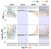 |
Fig. 7. As in Fig. 6 but for a γNFW = 0 fit. |
| In the text | |
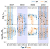 |
Fig. 8. As in Fig. 6 but for a γNFW = 1.5 fit. |
| In the text | |
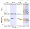 |
Fig. 9. As in Fig. 6 but for a γNFW = 2 fit. |
| In the text | |
Current usage metrics show cumulative count of Article Views (full-text article views including HTML views, PDF and ePub downloads, according to the available data) and Abstracts Views on Vision4Press platform.
Data correspond to usage on the plateform after 2015. The current usage metrics is available 48-96 hours after online publication and is updated daily on week days.
Initial download of the metrics may take a while.