| Issue |
A&A
Volume 691, November 2024
|
|
|---|---|---|
| Article Number | A336 | |
| Number of page(s) | 19 | |
| Section | Cosmology (including clusters of galaxies) | |
| DOI | https://doi.org/10.1051/0004-6361/202451123 | |
| Published online | 27 November 2024 | |
COMAP Pathfinder – Season 2 results
II. Updated constraints on the CO(1–0) power spectrum
1
Institute of Theoretical Astrophysics, University of Oslo,
PO Box 1029 Blindern,
0315
Oslo,
Norway
2
California Institute of Technology,
1200 E. California Blvd.,
Pasadena,
CA
91125,
USA
3
Canadian Institute for Theoretical Astrophysics, University of Toronto,
60 St. George Street,
Toronto,
ON
M5S 3H8,
Canada
4
Dunlap Institute for Astronomy and Astrophysics, University of Toronto,
50 St. George Street,
Toronto,
ON
M5S 3H4,
Canada
5
Department of Astronomy, Cornell University,
Ithaca,
NY
14853,
USA
6
Center for Cosmology and Particle Physics, Department of Physics, New York University,
726 Broadway,
New York,
NY
10003,
USA
7
Department of Physics, Southern Methodist University,
Dallas,
TX
75275,
USA
8
Departement de Physique Théorique, Universite de Genève,
24 Quai Ernest-Ansermet,
1211
Genève 4,
Switzerland
9
Owens Valley Radio Observatory, California Institute of Technology,
Big Pine,
CA
93513,
USA
10
Jodrell Bank Centre for Astrophysics, Alan Turing Building, Department of Physics and Astronomy, School of Natural Sciences, The University of Manchester,
Oxford Road,
Manchester
M13 9PL,
UK
11
Department of Physics and Astronomy, University of British Columbia, Vancouver,
BC
Canada
V6T 1Z1,
Canada
12
Jet Propulsion Laboratory, California Institute of Technology,
4800 Oak Grove Drive,
Pasadena,
CA
91109,
USA
13
Department of Physics, Korea Advanced Institute of Science and Technology (KAIST),
291 Daehak-ro, Yuseong-gu,
Daejeon
34141,
Republic of Korea
14
Department of Physics, University of Toronto,
60 St. George Street,
Toronto,
ON
M5S 1A7,
Canada
15
David A. Dunlap Department of Astronomy, University of Toronto,
50 St. George Street,
Toronto,
ON,
M5S 3H4,
Canada
16
Brookhaven National Laboratory,
Upton,
NY
11973-5000,
USA
17
Kavli Institute for Particle Astrophysics and Cosmology and Physics Department, Stanford University,
Stanford,
CA
94305,
USA
18
Department of Physics, University of Miami,
1320 Campo Sano Avenue,
Coral Gables,
FL
33146,
USA
19
Department of Astronomy, University of Maryland,
College Park,
MD
20742,
USA
★ Corresponding author; This email address is being protected from spambots. You need JavaScript enabled to view it.
Received:
14
June
2024
Accepted:
30
August
2024
Abstract
We present updated constraints on the cosmological 3D power spectrum of carbon monoxide CO(1–0) emission in the redshift range 2.4–3.4. The constraints are derived from the two first seasons of Carbon monOxide Mapping Array Project (COMAP) Pathfinder line intensity mapping observations aiming to trace star formation during the epoch of galaxy assembly. These results improve on the previous Early Science results through both increased data volume and an improved data processing methodology. On the methodological side, we now perform cross-correlations between groups of detectors (“feed groups”), as opposed to cross-correlations between single feeds, and this new feed group pseudo power spectrum (FGPXS) is constructed to be more robust against systematic effects. In terms of data volume, the effective mapping speed is significantly increased due to an improved observational strategy as well as a better data selection methodology. The updated spherically and field-averaged FGPXS, C~(k), is consistent with zero, at a probability-to-exceed of around 34%, with an excess of 2.7 σ in the most sensitive bin. Our power spectrum estimate is about an order of magnitude more sensitive in our six deepest bins across 0.09 Mpc−1 < k < 0.73 Mpc−1, compared to the feed-feed pseudo power spectrum (FPXS) of COMAP ES. Each of these bins individually constrains the CO power spectrum to k PCO(k) < 2400–4900 μK2Mpc2 at 95% confidence. To monitor potential contamination from residual systematic effects, we analyzed a set of 312 difference-map null tests and found that these are consistent with the instrumental noise prediction. In sum, these results provide the strongest direct constraints on the cosmological 3D CO(1–0) power spectrum published to date.
Key words: methods: data analysis / methods: observational / galaxies: high-redshift / diffuse radiation / radio lines: galaxies
© The Authors 2024
 Open Access article, published by EDP Sciences, under the terms of the Creative Commons Attribution License (https://creativecommons.org/licenses/by/4.0), which permits unrestricted use, distribution, and reproduction in any medium, provided the original work is properly cited.
This article is published in open access under the Subscribe to Open model. This email address is being protected from spambots. You need JavaScript enabled to view it. to support open access publication.
1 Introduction
By collecting the combined redshift-dependent line emission from all sources, both diffusely emitting gas and all galaxies, bright and faint, line intensity mapping (LIM) aims to map the Universe from large to small scales in three dimensions (see Madau et al. 1997; Battye et al. 2004; Peterson et al. 2006; Loeb & Wyithe 2008; Kovetz et al. 2017, 2019, and references therein for details on LIM). Several emission lines of interest have been proposed, among them 21 cm, carbon monoxide (CO), ionized carbon ([C II]), Lyα, and Hα, each with different astrophysical and cosmological goals (Kovetz et al. 2017, 2019; Bernal & Kovetz 2022).
At the forefront of CO LIM is the CO Mapping Array Project (COMAP), currently in its Pathfinder phase, which aims to measure the large-scale CO(1–0) line emission at redshifts of z ~ 2.4–3.4, tracing the star-forming galaxies around the epoch of galaxy assembly (Cleary et al. 2022). The COMAP Pathfinder instrument is a focal plane array of 19 detectors (which we refer to as “feeds”), each with independent receiver electronics, fielded on a 10.4 m Leighton telescope at the Owens Valley Radio Observatory. It observes in a frequency range of 26–34 GHz and is sensitive to 115.27 GHz CO(1–0) rotational line emission at redshifts of z ~ 2.4–3.4. Based on the first year of observations (“Season 1”), COMAP obtained the first direct limits on the 3D CO(1–0) clustering power spectrum, already ruling out several models from the literature. These results were published in a series of eight Early Science (ES) papers, along with a preview of our ongoing continuum survey of the Galaxy, a look at the prospects for CO LIM at the epoch of reionization, and a crosscorrelation of ES data with an overlapping galaxy survey (Cleary et al. 2022; Lamb et al. 2022; Foss et al. 2022; Ihle et al. 2022; Chung et al. 2022; Rennie et al. 2022; Breysse et al. 2022; Dunne et al. 2024).
In this paper, the second in a series of three, we update our power spectrum results based on observations taken in our first and second seasons (S2), following Ihle et al. (2022). We build on the filtered and calibrated low-level COMAP data products described in detail by Lunde et al. (2024). Implications for astrophysical constraints and modeling are explored by Chung et al. (2024a).
As is discussed by Lunde et al. (2024), the current experimental design is overall very similar to ES, but takes into account a few important lessons learned. For example, COMAP Season 2 uses only constant elevation scans (CES), not Lissajous scans, because one of the main conclusions of Ihle et al. (2022) was that changes in elevation within a scan result in significant residual systematic effects from changes in the atmospheric and or ground pickup signals. We also avoid elevations that are strongly contaminated by ground radiation received in the sidelobes. In addition, the instrument drive speed was decreased around May 2022 in order to reduce the stress on the telescope (Lunde et al. 2024), and the effective instrumental properties therefore changed notably about halfway through the second season. We denote periods before and after the speed change the “fast-” and “slow-moving azimuth scans” respectively (these are equivalent to the naming convention “Season 1+Season 2a” and “Season 2b” used by Lunde et al. (2024), where “a” and “b” denote the period before and after the drive changes).
For consistency with previous COMAP publications, we adopt the same ΛCDM cosmological model as Chung et al. (2022) and Li et al. (2016) when converting distances in our map cubes from angular and spectral frequency units into physical units. Explicitly we set Ωm = 0.286, ΩΛ = 0.714, Ωb = 0.047, H0 = 100 h km s−1 Mpc−1, h = 0.7, σ8 = 0.82, and ns = 0.96, which is roughly consistent with WMAP (Hinshaw et al. 2013). Unless otherwise stated all distances and distance-derived quantities in megaparsecs carry an implicit h−1.
This paper is structured as follows, the power spectrum methodology and updated null test framework are presented in Sect. 2 and 3 respectively. In Sect. 4, we present the power spectrum transfer function used to account for signal loss from low-level filtering and instrumental effects. Sections 5 and 6 show the power spectrum results and the outcome of our null tests. Our conclusions are presented in Sect. 7.
2 Power spectrum methodology
The power spectrum fully characterizes the information contained in a Gaussian random field and so is one of the most powerful statistics for cosmological density fields. While the non-linear physics of galactic emissions to which COMAP is sensitive is not fully Gaussian, the power spectrum is still a useful statistic, and complementary to other summary statistics such as the Voxel Intensity Distribution (VID); (Breysse et al. 2017; Ihle et al. 2019) or the Deconvolved Distribution Estimator (DDE); (Breysse et al. 2023; Chung et al. 2023).
The COMAP Pathfinder uses three-dimensional maps of the CO(1–0) emission to constrain models of star formation during the epoch of galaxy assembly. While the maps already represent the compression of hundreds of terabytes of raw time-ordered data (TOD) into only a few gigabytes, it is possible to encode and compress much of the relevant astrophysical and cosmological information contained within the maps even more by using summary statistics like the power spectrum. As such the power spectra are easier and more computationally efficient to work with when constraining astrophysical and cosmological information of the mapped emission field.
In the COMAP ES paper series, Ihle et al. (2022) devised a novel cross-power spectrum methodology, the feed-feed pseudo-cross-power spectrum (FPXS), constructed to be robust against systematic errors. This work largely builds on the methodology developed by Ihle et al. (2022) and lessons learned since the ES data processing to improve the power spectrum constraints of COMAP even further. In the following we summarize the FPXS methodology used and outline what has changed from the methodology developed by Ihle et al. (2022).
2.1 The feed group pseudo-cross-power spectrum
We begin by defining the general concepts of an auto- and cross-power spectrum. The auto-power spectrum can simply be defined as the variance of Fourier modes of a map. It can be written as
![Mathematical equation: $\[P(\boldsymbol{k})=\frac{V_{\mathrm{vox}}}{N_{\mathrm{vox}}}\langle | \mathcal{F}\{\boldsymbol{m}_{i}\}|^{2}\rangle=\frac{V_{\mathrm{vox}}}{N_{\mathrm{vox}}}\langle | f_{i}(\boldsymbol{k})|^{2}\rangle,\]$](/articles/aa/full_html/2024/11/aa51123-24/aa51123-24-eq2.png) (1)
(1)
where Vvox is the volume of a voxel (i.e., three-dimensional pixel) in units Mpc3, Nvox is the number of voxels and fi(k) are the Fourier coefficients of the map mi at wavenumber k. The units of fi(k) and k are, respectively, the same as the map’s mi and Mpc−1. For the Fourier transform ℱ{mi} of the map mi we use the same convention previously used in ES (Ihle et al. 2022; Harris et al. 2020). We can safely use the regular Fourier basis in the case of COMAP, instead of the more general spherical harmonics, as the fields are only ~2° in diameter and the flat-sky approximation is sufficient. Since our maps are three-dimensional, so is the power spectrum derived from those maps.
The auto-power spectrum will pick up all components that contribute to the variance in the map: signal, noise, and systematic effects. It can thus be decomposed into
![Mathematical equation: $\[P(\boldsymbol{k})=P_{\mathrm{CO}}(\boldsymbol{k})+P_{\text {noise}}(\boldsymbol{k})+P_{\text {syst}}(\boldsymbol{k}),\]$](/articles/aa/full_html/2024/11/aa51123-24/aa51123-24-eq3.png) (2)
(2)
showing contributions from CO signal1, noise and systematic effects, respectively. To obtain an unbiased estimate of the signal power spectrum, the systematic effects and noise properties of the map have to be understood and modeled.
Similarly to the auto-power spectrum, we can define a cross-power spectrum between two maps to be the covariance of Fourier coefficients of the two. It can be written as
![Mathematical equation: $\[C_{i j}(\boldsymbol{k})=\frac{V_{\mathrm{vox}}}{N_{\mathrm{vox}}}\left\langle\operatorname{Re}\{f_{i}^{*}(\boldsymbol{k}) f_{j}(\boldsymbol{k})\}\right\rangle,\]$](/articles/aa/full_html/2024/11/aa51123-24/aa51123-24-eq4.png) (3)
(3)
where fi and fj represent Fourier coefficients of two different maps i and j. The cross-power spectrum reduces to the auto-power spectrum if the two maps i and j are chosen to be identical.
As opposed to the auto-power spectrum, a cross-power spectrum will only be sensitive to correlated common modes between the two maps. Independent noise and independent systematic effects will therefore be canceled out and we can decompose the cross-spectrum as
![Mathematical equation: $\[C_{\mathrm{ij}}(\boldsymbol{k})=P_{\mathrm{CO}}(\boldsymbol{k})+C_{i j, \mathrm{common}}(\boldsymbol{k}),\]$](/articles/aa/full_html/2024/11/aa51123-24/aa51123-24-eq5.png) (4)
(4)
where Cij,common (k) represents the cross-spectrum contribution from some common systematic effect between the two maps.
We can now see a powerful property of the cross-spectrum: if we can choose two maps with independent noise properties and statistically unique systematic effects, giving Cij,common (k) = 0, the cross-power spectrum will yield an unbiased estimator for the signal power spectrum PCO(k).
This is the main property that the FPXS developed by Ihle et al. (2022) is built to exploit. Because the COMAP Pathfinder measures the sky with 19 feeds, each with its own receiver signal chain, the maps from different detectors will have independent noise properties. Additionally, several systematic effects are believed to be unique to each feed, or specific group of feeds. Therefore, a cross-spectrum between two detector maps will not be biased by the noise contribution of the detectors or feed-specific systematic contamination.
In this work, rather than cross-correlating individual feeds, we instead cross-correlate groups of feeds. In particular, we group feeds by their shared first down-conversion (DCM1) local oscillator (Lamb et al. 2022). Table 1 shows the feeds that are grouped together in a given “feed group”.
The reason for this change is that some of the systematic effects uncovered with the improved sensitivity of the current data volume are correlated with the DCM1 feed groups as has been shown by Lunde et al. (2024). Applying the original FPXS, involving cross-correlation of feeds from the same feed group, would not have been effective in canceling such systematic effects since they are common-mode for a given feed group.
Instead, by grouping all feeds in a given feed group together, detectors from the same feed group are never cross-correlated when computing the average feed group pseudo-cross-power spectra (FGPXS). This effectively cancels the systematic effects that are common to each feed group, while retaining the CO signal. Additionally, grouping together detectors in this way produces effective detector maps that have more sky overlap. Thus, when cross-correlating these maps we obtain better constraints on large-scale power spectrum modes and less mode-mixing due to a larger cross-map footprint. The result from a lower degree of mode mixing is also a lower amount of large-scale systematic effects that can leak into the small- and intermediate-scale power. This is especially important, as we know from Lunde et al. (2024) that our most dominant systematic effects are large-scale modes in the maps.
After splitting the data into feeds or feed groups, we split the data additionally into halves, each with independent systematic effect contributions, such as high or low elevation, as was done by Ihle et al. (2022). This further eliminates unwanted contributions to the cross-spectrum.
However, even though the FGPXS is slightly more robust to systematic effects, this comes at the price of a slight decrease in sensitivity. The expected loss in sensitivity when using FGPXS as opposed to FPXS should in theory follow the upper limit found by Ihle et al. (2022):
![Mathematical equation: $\[\sigma_{C(\boldsymbol{k})}^{N_{\text {split}}, N_{\text {feed}}} \geq \sqrt{\frac{1}{1-\frac{1}{N_{\text {split}}}}} \sqrt{\frac{1}{1-\frac{1}{N_{\text {feed}}}}} \sigma_P(k)\]$](/articles/aa/full_html/2024/11/aa51123-24/aa51123-24-eq6.png) (5)
(5)
![Mathematical equation: $\[\stackrel{N_{\text {split}}=2}{=} \sqrt{\frac{2}{1-\frac{1}{N_{\text {feed}}}}} \sigma_P(k),\]$](/articles/aa/full_html/2024/11/aa51123-24/aa51123-24-eq7.png) (6)
(6)
where the uncertainty of a cross-spectrum, ![Mathematical equation: $\[\sigma_{C(\boldsymbol{k})}^{N_{\text {spit}}, N_{\text {feed }}}\]$](/articles/aa/full_html/2024/11/aa51123-24/aa51123-24-eq8.png) , is given by the number of cross-correlated data splits and feeds, Nsplit and Nfeed, compared to the optimal sensitivity, σP(k), one can obtain when using all available data in an auto-power spectrum. To incorporate the effects of both cross-correlating feeds and an additional cross-variable on the total sensitivity we have generalized Eq. (14) of Ihle et al. (2022) to obtain Eq. (5). Because we use the same elevation split as Ihle et al. (2022), splitting the data into high or low elevation, the Nsplit dependency of Eq. (5) reduces to the
, is given by the number of cross-correlated data splits and feeds, Nsplit and Nfeed, compared to the optimal sensitivity, σP(k), one can obtain when using all available data in an auto-power spectrum. To incorporate the effects of both cross-correlating feeds and an additional cross-variable on the total sensitivity we have generalized Eq. (14) of Ihle et al. (2022) to obtain Eq. (5). Because we use the same elevation split as Ihle et al. (2022), splitting the data into high or low elevation, the Nsplit dependency of Eq. (5) reduces to the ![Mathematical equation: $\[\sqrt{2}\]$](/articles/aa/full_html/2024/11/aa51123-24/aa51123-24-eq9.png) loss in sensitivity in Eq. (6).
loss in sensitivity in Eq. (6).
To give some intuition on Eq. (5), we show a grid of possible feed group and elevation split combinations in Fig. 1. Equation (6) can be obtained by using a grid like the one seen in Fig. 1 from the ratio between the total number of split combinations (i.e. the optimal auto-spectrum sensitivity σP) and the number of all cross-combinations that do not constitute autocombinations between feeds or elevations (respectively dark and light gray shading). From this we should expect there to be a loss in sensitivity in the FGPXS compared to FPXS of ~12% – that is by, respectively, inserting values for the number Nfeed of feed groups, Nfeed = 4, and all individual feeds, Nfeed = 19, in Eq. (6) and comparing the results2.
Nevertheless, we conservatively cluster feeds into the aforementioned feed groups to avoid systematic effect contamination, at the price of a minor loss in sensitivity. Apart from the reasons stated above, there is in principle no difference between the FPXS and FGPXS algorithmically; for instance, it would be trivial to group the feeds in a different configuration if that were found to be advantageous in the future for some reason. We can thus describe the two methods using the same algorithmic representation shown in the following. We can write the main steps of the FGPXS algorithmically as follows:
Split the data into two halves A and B. As was done by Ihle et al. (2022), we chose elevation as the main crosscorrelation variable to eliminate potential sidelobe pickup from the ground.
For parts A and B respectively make maps of each feed group i. We denote these by, for example,
![Mathematical equation: $\[m_{A_{2}}\]$](/articles/aa/full_html/2024/11/aa51123-24/aa51123-24-eq10.png) for a map of part A with feed group 2.
for a map of part A with feed group 2.For each combination of feed groups i and j, and data splits A and B, compute cross-power spectra.
-
Compute a noise-weighted average FGPXS of all the resulting Nfeedgroup × (Nfeedgroup – 1) (with Nfeedgroup = 4 when using feed groups and Nfeedgroup = 19 if computing the ES FPXS) individual FGPXS that do not involve the same detector or elevation:
![Mathematical equation: $\[C(\boldsymbol{k})=\frac{\sum_{A_i \neq B_j} \frac{C_{A_i B_j}(\boldsymbol{k})}{{\sigma_{C_{A_i B_j}}^2(\boldsymbol{k}})}}{\sum_{A_i \neq B_j} \frac{1}{\sigma_{C_{A_i B_j}}^2(\boldsymbol{k})}},\]$](/articles/aa/full_html/2024/11/aa51123-24/aa51123-24-eq11.png) (7)
(7)with a corresponding uncertainty of
![Mathematical equation: $\[\sigma_{C(k)}=\frac{1}{\sqrt{\sum_{A_i \neq B_j} \frac{1}{\sigma_{C_{A_i B_j}}^2(k)}}}.\]$](/articles/aa/full_html/2024/11/aa51123-24/aa51123-24-eq12.png) (8)
(8)This is what we refer to as the mean feed group pseudo-cross-power spectrum (FGPXS) or feed-feed pseudo-cross-power spectrum (FPXS), if (respectively) feed groups or feeds are used as effective detectors.
In Fig. 1, we illustrate a grid of possible feed group and elevation combinations used for an average FGPXS. Those shaded dark and light gray represent auto-feed and auto-elevation combinations (respectively). The combinations that cross neither feed groups nor elevations, indicated with examples of 2D FGPXS combinations, are used in the final average FGPXS in Eq. (7).
Due to the non-uniform coverage of our sky fields, as well as a non-trivial survey footprint (see Lunde et al. 2024, for examples of maps), the maps are weighted prior to computing their Fourier coefficients. We use the same weighting scheme as Ihle et al. (2022), given for a cross-power spectrum by
![Mathematical equation: $\[\boldsymbol{w}_{A_{i} B_{j}} \propto \frac{1}{\sigma_{A_{i}} \sigma_{B_{j}}},\]$](/articles/aa/full_html/2024/11/aa51123-24/aa51123-24-eq13.png) (9)
(9)
where ![Mathematical equation: $\[\boldsymbol{\sigma}_{Y_{x}}\]$](/articles/aa/full_html/2024/11/aa51123-24/aa51123-24-eq14.png) represents the uncertainty estimate in each voxel of a feed group and elevation split map,
represents the uncertainty estimate in each voxel of a feed group and elevation split map, ![Mathematical equation: $\[\boldsymbol{m}_{Y_{x}}\]$](/articles/aa/full_html/2024/11/aa51123-24/aa51123-24-eq15.png) . These weights are then applied to the map,
. These weights are then applied to the map, ![Mathematical equation: $\[\tilde{\boldsymbol{m}}_{i}=\boldsymbol{w}_{i} \boldsymbol{m}_{i}\]$](/articles/aa/full_html/2024/11/aa51123-24/aa51123-24-eq16.png) , before power spectrum estimation with the Fourier coefficients
, before power spectrum estimation with the Fourier coefficients ![Mathematical equation: $\[\tilde{f}_{i}(\boldsymbol{k})=\mathcal{F}\{\boldsymbol{w}_{i} \boldsymbol{m}_{i}\}\]$](/articles/aa/full_html/2024/11/aa51123-24/aa51123-24-eq17.png) in Eq. (3). Regions outside the map footprints are assigned zero weights. The power spectra of these weighted maps are commonly referred to as pseudo power spectra (Hivon et al. 2002). The pseudo power spectra are a biased power spectrum estimator because different Fourier modes become coupled via the applied weights (see Hivon et al. 2002; Leung et al. 2022, for details on mode mixing). It should be noted that we use
in Eq. (3). Regions outside the map footprints are assigned zero weights. The power spectra of these weighted maps are commonly referred to as pseudo power spectra (Hivon et al. 2002). The pseudo power spectra are a biased power spectrum estimator because different Fourier modes become coupled via the applied weights (see Hivon et al. 2002; Leung et al. 2022, for details on mode mixing). It should be noted that we use ![Mathematical equation: $\[\tilde{P}(k)\]$](/articles/aa/full_html/2024/11/aa51123-24/aa51123-24-eq18.png) to denote pseudo spectra in the later results sections, but we use the notation P(k) (without the tilde) in the methods sections as most of the methodology is equivalently written for unbiased and pseudo spectra. A detailed discussion of the COMAP-specific mode mixing can be found in Fig. 1 and Appendix D of Ihle et al. (2022), which shows that the effect is ≤20% over our k-range. Reversing the mode-mixing will thus be left as a future exercise and is beyond the scope of this work.
to denote pseudo spectra in the later results sections, but we use the notation P(k) (without the tilde) in the methods sections as most of the methodology is equivalently written for unbiased and pseudo spectra. A detailed discussion of the COMAP-specific mode mixing can be found in Fig. 1 and Appendix D of Ihle et al. (2022), which shows that the effect is ≤20% over our k-range. Reversing the mode-mixing will thus be left as a future exercise and is beyond the scope of this work.
Feed groups used in the feed group pseudo-cross-power spectrum.
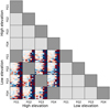 |
Fig. 1 Example grid of possible feed group (FG1–4) and elevation (high and low) split combinations. Combinations with dark and light gray shading, respectively, represent auto-feed group and auto-elevation combinations that are not used in the final averaged FGPXS. The crosscombinations containing examples of a 2D cross-spectrum contribute to the final average FGPXS as neither identical feed groups, nor elevations, are crossed. |
2.2 The binned power spectrum estimator
As COMAP produces line intensity maps spanning threedimensional redshift-space volumes, the resulting power spectra also span three-dimensional Fourier-space volumes. It can, however, be easier to work with a power spectrum spherically averaged down to one dimension. For the spherically averaged power spectrum to contain all relevant information in the full three-dimensional power spectrum, the emission field is technically required to remain statistically isotropic on large scales and stationary across the mapped redshift range. This is not strictly known to be true for the CO emission field. Cosmic star-formation, especially dust-obscured star-formation history traced in the infrared, is poorly constrained in our targeted redshift range of z = 2.4–3.4 (see Madau & Dickinson 2014, for a review of cosmic star-formation history). As a consequence, the extent to which the mapped CO emission field is stationary is largely unknown. The spherically averaged power spectrum of a dynamic field will not be sensitive to changes in the CO emission across cosmic time, but it will measure the time-averaged properties of the targeted CO structures. However, the distinction is moot for the current COMAP signal-to-noise ratio (S/N), as no clear CO excess is observed in the power spectra. Thus we present the spherically averaged, 1D power spectrum as our main science product.
Additionally, in practice, the angular and the redshift axes are observed in fundamentally different ways, and the low-level filtering applied to the data (Lunde et al. 2024) as well as redshift space distortions and line-broadening (Chung et al. 2021) can affect the signal and sensitivity differently along each axis. Therefore, the angular and line-of-sight dimensions are convenient to separate, and we bin the 3D power spectrum C(k), with k = (kx, ky, kz), into both a cylindrical and spherically averaged power spectrum. The former of these conserves the structures perpendicular and parallel to the line-of-sight by only merging the two angular axes
![Mathematical equation: $\[\boldsymbol{k}_{i}=\left(k_{\perp}, k_{\|}\right)=\left(\sqrt{k_{x}^{2}+k_{y}^{2}}, k_{z}\right).\]$](/articles/aa/full_html/2024/11/aa51123-24/aa51123-24-eq19.png) (10)
(10)
Meanwhile, the latter will average the 3D power spectrum into 1D bins of the form
![Mathematical equation: $\[k_{i}=\sqrt{k_{x}^{2}+k_{y}^{2}+k_{z}^{2}}.\]$](/articles/aa/full_html/2024/11/aa51123-24/aa51123-24-eq20.png) (11)
(11)
The binned cylindrically averaged power spectrum estimator will then become
![Mathematical equation: $\[C(\boldsymbol{k}) \approx C_{\boldsymbol{k}_{i}}=\frac{V_{\mathrm{vox}}}{N_{\mathrm{vox}} N_{\text {modes }}} \sum_{\boldsymbol{k} \in k_{i}}\left\langle\operatorname{Re}\left\{f_{1}^{*}(\boldsymbol{k}) f_{2}(\boldsymbol{k})\right\}\right\rangle,\]$](/articles/aa/full_html/2024/11/aa51123-24/aa51123-24-eq21.png) (12)
(12)
where the number of Fourier modes in bin ki is given as Nmodes. The equation is completely analogous when binning to the spherically averaged power spectrum. We henceforth refer to the cylindrically and spherically averaged power spectrum estimators as “2D” and “1D” due to the number of axes needed to display them, but note that they still represent averages of a 3D density field.
The bin edges are chosen to cover the scales to which COMAP is most sensitive and correspond to those used in the COMAP ES power spectra (Ihle et al. 2022), but due to our large increase in sensitivity and better understanding of the origin of correlations on large angular scales we conservatively excise all perpendicular scales k⊥ ≲ 0.1 Mpc−1 for this publication. On these scales, we are dominated by sub-optimal cross-map overlap that results in poor constraining power of the large-scale structure as well as the possibility of large-scale residual systematic effect leakage through mode mixing into the small-scale power spectrum modes (see Lunde et al. 2024, for examples of our map-domain systematic effects). In the future, we aim to recover the large scales at k⊥ ≲ 0.1 Mpc−1. Lastly, we also mask the bins corresponding to the highest k⊥ and k∥ used by Ihle et al. (2022) to prevent issues with aliasing near the Nyquist frequency of the two respective dimensions: ![Mathematical equation: $\[k_{\perp}^{\text {Nyquist }} \approx 1.22 ~\mathrm{Mpc}^{-1}\]$](/articles/aa/full_html/2024/11/aa51123-24/aa51123-24-eq22.png) and
and ![Mathematical equation: $\[k_{\|}^{\text {Nyquist }} \approx 0.74 ~\mathrm{Mpc}^{-1}\]$](/articles/aa/full_html/2024/11/aa51123-24/aa51123-24-eq23.png) .
.
2.3 Uncertainty estimation from randomized null maps
In order to compute the mean FGPXS and its errors, as is shown in Eqs. (7) and (8), we need the power spectrum uncertainties for each feed group and elevation cross-combination, ![Mathematical equation: $\[\sigma_{C_{A_{i} B_{j}}}^{2}(\boldsymbol{k})\]$](/articles/aa/full_html/2024/11/aa51123-24/aa51123-24-eq24.png) . This can be done via two basic approaches: simulations and data-driven methods. Here, we first detail some problems with a simulation-based approach used previously in COMAP ES (Ihle et al. 2022) and subsequently argue for why a data-driven approach was chosen in this work.
. This can be done via two basic approaches: simulations and data-driven methods. Here, we first detail some problems with a simulation-based approach used previously in COMAP ES (Ihle et al. 2022) and subsequently argue for why a data-driven approach was chosen in this work.
In COMAP ES, Ihle et al. (2022) chose a simple simulation approach where the power spectrum uncertainties were computed from an ensemble of simple white noise maps, mnoise,i ~ 𝒩(0, σ), drawn from a zero-mean Gaussian distribution 𝒩 with the voxel uncertainties σ. These were then propagated to the power spectrum level. The main advantage of this approach is its computational efficiency. However, it can only reflect the white noise level within the map, while residual correlated noise and the effect of the pipeline filters on the noise will not be contained in the uncertainty from these simple white noise maps (see, for instance, the power spectral density (PSD) of TOD in Fig. 9 of Lunde et al. 2024, for an illustration of the noise properties of the filtered data). The simplified simulations proved an adequate method given the sensitivity of our ES data. With the increased sensitivity achieved at the end of S2, obtaining suitable power spectrum errors, ![Mathematical equation: $\[\sigma_{C_{k}}\]$](/articles/aa/full_html/2024/11/aa51123-24/aa51123-24-eq25.png) , through simulations would require the sampling of noise from the TOD domain (ideally with additional ground-up modeling of all contributing systematic effects), propagating it all the way through the low-level pipeline (Lunde et al. 2024) up to the power spectrum. However, this would be computationally expensive because the low-level pipeline filters would have to be re-run for each ensemble, and require significant additional data modeling.
, through simulations would require the sampling of noise from the TOD domain (ideally with additional ground-up modeling of all contributing systematic effects), propagating it all the way through the low-level pipeline (Lunde et al. 2024) up to the power spectrum. However, this would be computationally expensive because the low-level pipeline filters would have to be re-run for each ensemble, and require significant additional data modeling.
Given the drawbacks of both the white noise and a potential TOD-level simulation-based approach, a data-driven method was instead chosen for this work as it represents a relatively computationally inexpensive method of estimating the power spectrum uncertainties that automatically reflects all the properties of the data. In particular, we draw from the simple idea that we can cancel the signal and systematic effects in a subtraction between data-half maps while leaving the correct noise properties. In our case, we estimate ![Mathematical equation: $\[\sigma_{C_{k}}\]$](/articles/aa/full_html/2024/11/aa51123-24/aa51123-24-eq26.png) by what we refer to as an ensemble of randomized null difference (RND) maps.
by what we refer to as an ensemble of randomized null difference (RND) maps.
The first step in the RND calculation is to divide the set of all scans in the data into two randomized halves, A and B, from which we subsequently make maps ![Mathematical equation: $\[\boldsymbol{m}_{A, i}^{\mathrm{RND}}\]$](/articles/aa/full_html/2024/11/aa51123-24/aa51123-24-eq27.png) and
and ![Mathematical equation: $\[\boldsymbol{m}_{B, i}^{\mathrm{RND}}\]$](/articles/aa/full_html/2024/11/aa51123-24/aa51123-24-eq28.png) . This is done for all random split realizations i. Both
. This is done for all random split realizations i. Both ![Mathematical equation: $\[\boldsymbol{m}_{A, i}^{\mathrm{RND}}\]$](/articles/aa/full_html/2024/11/aa51123-24/aa51123-24-eq29.png) and
and ![Mathematical equation: $\[\boldsymbol{m}_{B, i}^{\mathrm{RND}}\]$](/articles/aa/full_html/2024/11/aa51123-24/aa51123-24-eq30.png) should contain the same signal, and due to the randomization of the splits also the same systematic effects. Hence we can cancel both the signal and systematic effects by computing the difference between the two maps;
should contain the same signal, and due to the randomization of the splits also the same systematic effects. Hence we can cancel both the signal and systematic effects by computing the difference between the two maps;
![Mathematical equation: $\[\Delta \boldsymbol{m}_{i}^{\mathrm{RND}}=\frac{\boldsymbol{m}_{A, i}^{\mathrm{RND}}-\boldsymbol{m}_{B, i}^{\mathrm{RND}}}{2}.\]$](/articles/aa/full_html/2024/11/aa51123-24/aa51123-24-eq31.png) (13)
(13)
The difference maps ![Mathematical equation: $\[\Delta \boldsymbol{m}_{i}^{\mathrm{RND}}\]$](/articles/aa/full_html/2024/11/aa51123-24/aa51123-24-eq32.png) now optimally capture the white and correlated noise properties and biases (from low-level filters, the instrumental beam, etc.) of the real maps, but are without any of the signal or systematic effects. As such they reflect the true properties of the data to a high degree.
now optimally capture the white and correlated noise properties and biases (from low-level filters, the instrumental beam, etc.) of the real maps, but are without any of the signal or systematic effects. As such they reflect the true properties of the data to a high degree.
Finally, to obtain the uncertainty of the power spectrum ![Mathematical equation: $\[\sigma_{C_{k}}\]$](/articles/aa/full_html/2024/11/aa51123-24/aa51123-24-eq33.png) we need to compute the FGPXS of each difference map
we need to compute the FGPXS of each difference map ![Mathematical equation: $\[\Delta \boldsymbol{m}_{i}^{\mathrm{RND}}\]$](/articles/aa/full_html/2024/11/aa51123-24/aa51123-24-eq34.png) . From the resulting ensemble of such feed group cross-spectra,
. From the resulting ensemble of such feed group cross-spectra, ![Mathematical equation: $\[C_{\Delta m_{i}}^{\mathrm{RND}}(\boldsymbol{k})\]$](/articles/aa/full_html/2024/11/aa51123-24/aa51123-24-eq35.png) , we can compute the uncertainties σRND(k) by taking the standard deviation over the ensemble. These can then be used when co-adding together feed group spectra to obtain the final mean FGPXS as is explained in Eqs. (7) and (8).
, we can compute the uncertainties σRND(k) by taking the standard deviation over the ensemble. These can then be used when co-adding together feed group spectra to obtain the final mean FGPXS as is explained in Eqs. (7) and (8).
3 Power spectrum null tests
With the increased effective COMAP data volume and the resulting increased sensitivity comes the need for more effective null tests to ensure the data quality of our final power spectra.
As we explain in this section, the null tests devised in this work are based on difference maps in a similar way to the RND method used for uncertainty estimation described earlier in Sect. 2.3, except we are now splitting the maps on meaningful parameters instead of randomly. The goal then becomes finding null variables (e.g. high or low humidity or left or right moving scans; see Table C.2 for a list of all chosen variables) that correlate to systematic effects in one of the null variable halves by which we split the data.
We can write the difference map of some null variable j as
![Mathematical equation: $\[\Delta \boldsymbol{m}_{j}^{\text {null }}=\frac{\boldsymbol{m}_{A, j}-\boldsymbol{m}_{B, j}}{2},\]$](/articles/aa/full_html/2024/11/aa51123-24/aa51123-24-eq36.png) (14)
(14)
where the maps mA,j and mB,j represent the maps of the two halves of the data respectively. If the chosen null variable correlates to a systematic effect, the difference map ![Mathematical equation: $\[\Delta \boldsymbol{m}_{j}^{\text {null }}\]$](/articles/aa/full_html/2024/11/aa51123-24/aa51123-24-eq37.png) will contain the systematic effect but cancel the signal. The difference maps can then be used to perform a null test, with the null hypothesis being that the null maps are consistent with the general noise properties of the maps. The associated voxel uncertainty of the null map is then given by
will contain the systematic effect but cancel the signal. The difference maps can then be used to perform a null test, with the null hypothesis being that the null maps are consistent with the general noise properties of the maps. The associated voxel uncertainty of the null map is then given by
![Mathematical equation: $\[\sigma_{\Delta m_{j}}^{\mathrm{null}}=\frac{\sqrt{\sigma_{m_{A, j}}^{2}+\sigma_{m_{B, j}}^{2}}}{2},\]$](/articles/aa/full_html/2024/11/aa51123-24/aa51123-24-eq38.png) (15)
(15)
for uncertainties ![Mathematical equation: $\[\sigma_{m_{A, j}}\]$](/articles/aa/full_html/2024/11/aa51123-24/aa51123-24-eq39.png) and
and ![Mathematical equation: $\[\sigma_{m_{B, j}}\]$](/articles/aa/full_html/2024/11/aa51123-24/aa51123-24-eq40.png) of the maps mA,j and mB,j respectively.
of the maps mA,j and mB,j respectively.
For each of the null variables j we then take the difference between the two maps as is described by Eqs. (14) and (15). As we use a cross-elevation FGPXS we must compute a difference map for both high and low elevation. The data are therefore split into four parts, two elevation ranges and two null variables halves, where we subtract across the latter in the map domain and cross-correlate the resulting null maps across the former using the FGPXS method described earlier. With the set of resulting null test FGPXS ![Mathematical equation: $\[C_{\Delta m_{j}}^{k_{i}}\]$](/articles/aa/full_html/2024/11/aa51123-24/aa51123-24-eq41.png) we can perform a χ2-test, with a null hypothesis that the difference maps are consistent with noise, by first computing
we can perform a χ2-test, with a null hypothesis that the difference maps are consistent with noise, by first computing
![Mathematical equation: $\[\chi_{\text {null }, j}^{2}=\sum_{k_{i}}\left(\frac{C_{\Delta m_{j}}^{k_{i}}-\mu_{\Delta m_{j}}^{k_{i}}}{\sigma_{C_{\Delta m_{j}}^{k_{i}}}}\right)^{2}=\sum_{k_{i}}\left(\frac{C_{\Delta m_{j}}^{k_{i}}}{\sigma_{C_{\Delta m_{j}}^{k_{i}}}}\right)^{2},\]$](/articles/aa/full_html/2024/11/aa51123-24/aa51123-24-eq42.png) (16)
(16)
with the expectation value of the null FGPXS ![Mathematical equation: $\[\mu_{\Delta m_{j}}^{k_{i}}=0\]$](/articles/aa/full_html/2024/11/aa51123-24/aa51123-24-eq43.png) under the null hypothesis. Here
under the null hypothesis. Here ![Mathematical equation: $\[\sigma_{C_{\Delta m_{j}}^{k_{i}}}\]$](/articles/aa/full_html/2024/11/aa51123-24/aa51123-24-eq44.png) is the uncertainty of the null FGPXS
is the uncertainty of the null FGPXS ![Mathematical equation: $\[C_{\Delta m_{j}}^{k_{i}}\]$](/articles/aa/full_html/2024/11/aa51123-24/aa51123-24-eq45.png) in bin ki for null variable j that is estimated using the RND method described earlier in Sect. 2.3.
in bin ki for null variable j that is estimated using the RND method described earlier in Sect. 2.3.
Thereafter we can compute the probability-to-exceed (PTE) that quantifies the probability of obtaining a value ![Mathematical equation: $\[\chi_{\text {null,}j }^{2}\]$](/articles/aa/full_html/2024/11/aa51123-24/aa51123-24-eq46.png) or higher. The PTE is defined as
or higher. The PTE is defined as
![Mathematical equation: $\[\operatorname{PTE}\left(\chi^{2}\right)=1-\operatorname{CDF}\left(\chi^{2}\right),\]$](/articles/aa/full_html/2024/11/aa51123-24/aa51123-24-eq47.png) (17)
(17)
where for a given probability distribution function P(χ2) of the ![Mathematical equation: $\[\chi_{\text {null}, j}^{2}\]$](/articles/aa/full_html/2024/11/aa51123-24/aa51123-24-eq48.png) values the corresponding cumulative distribution function is denoted as CDF(χ2).
values the corresponding cumulative distribution function is denoted as CDF(χ2).
In our case, P(χ2) does not follow the usual analytical χ2-distribution because the noise properties of the FGPXS are not completely known analytically (see Watts et al. 2020; Nadarajah & Pogány 2016; Gaunt 2019, for some examples of how crossspectrum noise properties can look). We thus compute the PTEs numerically by using an ensemble of RND maps equivalent to those we already use for estimating uncertainties as these will perfectly reflect the noise properties and biases in the data, as well as obey the null hypothesis. For each separate processing run – over fields, fast- and slow-moving azimuth data – we compute 244 RND maps, of which we use 61 for power spectrum uncertainty estimation and the remaining 183 for measuring the numerical χ2-distribution.
4 Transfer functions
As is described by Foss et al. (2022) and Ihle et al. (2022) the COMAP maps are not unbiased as the low-level filtering of the data, the binning of the data into voxels, and the finite resolution of the telescope beam will attenuate the signal in the maps. In this section, we explain how we de-bias our power spectrum estimates using transfer functions for each of the main effects that result in signal loss. The beam and voxel window smoothing of the signal is corrected using analytically computed transfer functions, while the low-level filtering attenuation is quantified using simulations. Details on how each transfer function is estimated are discussed by Lunde et al. (2024).
When performing a power spectrum analysis of our maps, as is described in Sect. 2, we obtain an estimate of the signal that is biased by several different effects. To see how the signal is biased we can write the FGPXS signal estimator as
![Mathematical equation: $\[C_{\boldsymbol{k}}=T(\boldsymbol{k}) P_{k}^{\mathrm{CO}}=T_{f}(\boldsymbol{k}) T_{\mathrm{b}}\left(k_{\perp}\right) T_{p}\left(k_{\perp}\right) T_{\nu}\left(k_{\|}\right) P_{k}^{\mathrm{CO}},\]$](/articles/aa/full_html/2024/11/aa51123-24/aa51123-24-eq49.png) (18)
(18)
where the transfer function T(k) is the product of the filter transfer function Tf(k), the beam smoothing transfer function Tb(k⊥) as well as the pixel and spectral channel windows, Tp(k⊥) and Tν(k∥). The transfer function can be written in this multiplicative form in the Fourier domain because the low-level filtering and the smoothing of small-scale structures due to the instrumental beam and voxel window of the map grid can all (approximately) be expressed as a convolution in map domain. In Fig. 2 we show the full transfer function product T(k), while the individual transfer function elements are shown in detail in Sect. 6. of Lunde et al. (2024).
Using our transfer function estimate we can de-bias the FGPXS by deconvolution;
![Mathematical equation: $\[P_{k}^{\mathrm{CO}}=\frac{C_{k}}{T(\boldsymbol{k})},\]$](/articles/aa/full_html/2024/11/aa51123-24/aa51123-24-eq50.png) (19)
(19)
with the uncertainties of the signal estimator being affected in a similar manner,
![Mathematical equation: $\[\sigma_{P_{k}}^{\mathrm{CO}}=\frac{\sigma_{C_{k}}}{T(\boldsymbol{k})},\]$](/articles/aa/full_html/2024/11/aa51123-24/aa51123-24-eq51.png) (20)
(20)
becoming large whenever the transfer function T(k) becomes small.
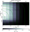 |
Fig. 2 Full power spectrum transfer function used to account for the signal losses due to the low-level filtering pipeline, the instrumental beam smoothing, and the voxel window of the maps (see Lunde et al. 2024, for details on each individual transfer function). Thin green contours indicate the bin edges of the (1D) spherically averaged FGPXS. |
5 Power spectrum results
In this section, we present the main power spectrum results of this paper. The raw data going into the power spectra are filtered, calibrated, and binned into maps after a set of data selection steps that remove scans that are likely contaminated by systematic effects. This is described in detail by Lunde et al. (2024).
As one of the main lessons learned from COMAP ES was to employ only CES scans, and no longer use a Lissajous scanning strategy, the data presented here consist only of CES data (Foss et al. 2022; Ihle et al. 2022). Specifically, we include all data obtained up to November 2023, both the ES (Season 1) CES data as well as all data gathered in S2. The data volume obtained in S2 is, as has been explained by Lunde et al. (2024), effectively around eight times larger than the Season 1 CES data after data selection. In addition, the ES analysis of Season 1 data excluded several detectors that were either offline or excluded due to clear signs of systematic excess in reduced χ2-tests or in visual inspections of feed cross-spectra. We are able to include these in the S2 analysis because all feeds were functioning during S2 and the map-domain PCA described in Lunde et al. (2024) strongly suppresses detector-specific systematic effects.
We note that in the ES analysis Ihle et al. (2022) removed feed-feed cross-spectra both through a reduced χ2-test, and manual inspection of misbehaving feed combinations. Due to better low-level data processing, we were able to remove all data-driven cuts in the power spectrum domain, with the increased set of null tests since ES working as an additional safeguard against systematic effects (see Sect. 6 for discussion of null test results).
Lastly, in Appendix D, we show a simple end-to-end signal injection test as a qualitative test of our pipeline’s ability to recover a known signal’s amplitude within the estimated experimental errors and power spectrum transfer function.
5.1 The cylindrically averaged power spectrum result
In Fig. 3, we show the cylindrically averaged (2D) mean FGPXS for all three fields separately, as well as in combination. The figure also shows the sensitivity per (k⊥, k∥)-bin as well as the FGPXS in units of the sensitivity.
When looking at the 2D FGPXS in Fig. 3 we note that the noise blows up on small scales, particularly so in the angular direction, due to the COMAP transfer function seen in Fig. 2 (Lunde et al. 2024). However, we see no obvious patterns in the 2D FGPXS that would indicate a systematic effect. In fact, the spectra resemble white noise.
As was mentioned earlier, in Sect. 2.2, we want to avoid issues with poorly constrained large-scale modes, strong mode mixing, and possible residual large-scale systematic effects. We mitigate these issues by excluding 2D bins at k⊥ < 0.1 Mpc−1. An example of spurious fluctuations induced by poor overlap can be seen in the COMAP ES cylindrically averaged FPXS of Field 1 (see Ihle et al. 2022, noting that Field 1 is especially susceptible to poor detector overlap due to its position at declination zero) as correlated structures along constant k⊥ at scales k⊥ < 0.1 Mpc−1. These correlations have since been understood to originate from sub-optimal detector overlap, and are pushed to larger scales due to a larger sky overlap when computing cross-spectra between feed groups instead of individual feeds. In interim estimates we found the average of the maximum correlations between a bin and all the others to be around 15% at scales k⊥ ≥ 0.1 Mpc−1, while the correlations at k⊥ ≤ 0.1 Mpc−1 are somewhere in the 30–70% regime. Improved modeling of these correlations will be the aim of future work.
5.2 The spherically averaged power spectrum result
As interpreting the 2D cylindrically averaged FGPXS can be somewhat unintuitive we can bin the spectra into 1D by performing a full spherical averaging. This is done as is described in Sect. 2.2, in which the 1D bin-edges are indicated as thin green contours in Fig. 3. When doing so we obtain the spherically averaged FGPXS for the three fields, as well as the combination thereof, as is seen in Fig. 4.
As was discussed in Sect. 5.1, we excluded scales k⊥ < 0.1 Mpc−1 from the power spectrum analysis to avoid issues with poor cross-map overlap, mode mixing and large correlations between large scale bins. Therefore, Fig. 4 only shows FGPXS data points on scales k > 0.1 Mpc−1. Similar to the discussion in Sect. 5.1, we estimate the average of the maximum correlation between a 1D bin and all the others, on scales k > 0.1 Mpc−1, to be ≲ 10% after excluding the large k⊥ scales and performing the spherical averaging. Given this ≲ 10% level, we shall assume for Season 2 analyses downstream that the spherically averaged 1D FPGXS bins are approximately uncorrelated. As with the 2D FGPXS discussed in Sect. 5.1, we intend to improve the exact modeling of these correlations in future work.
When looking at Fig. 4 we note that Fields 2 and 3 have the highest sensitivity, while Field 1 has around 50% larger errors than the two other fields. This is because, of the three COMAP fields, Field 1 is most affected by the low-level data cuts (see Lunde et al. 2024), and due to its location at zero declination, is particularly susceptible to poor detector overlap. In addition, by rejecting poorly overlapping detector combinations, which are also the least sensitive, we prevent the resulting strong mode mixing and potential consequent leakage of systematic effects into smaller scales at the cost of a relatively minimal loss in sensitivity. As a consequence, we keep 2/3 of the feed group cross-spectra of Field 1 in the analysis.
As we can see from Fig. 4, the cross-spectra are largely consistent with zero to within 2σ in most bins. However, perhaps the most notable feature is the high power in the second and most sensitive k-bin, at 0.12 Mpc−1 < k < 0.18 Mpc−1, which is respectively at around 2.3σ and 3σ significance above zero for Fields 1 and 2. Meanwhile, for Field 3 the same bin is consistent with zero power. When combining the three fields, the co-added data point in the second k-bin has a value that is 2.7σ away from zero. For each of the spherically averaged FGPXS of the three fields, we compute their χ2 PTE to check their constancy with zero power. In doing so, we obtain PTEs of, respectively, 33.2%, 19.5%, and 82.7% for Fields 1–3. The fieldcombined spherically averaged FGPXS results in a 34% PTE. As for the null tests, the PTE is estimated from the numerical RND χ2 ensemble. While the combined 1D ~2.7σ power in 0.12 Mpc−1 < k < 0.18 Mpc−1 bin is interesting, we do not consider it a statistically significant excess given the estimated PTEs. Thus, we shall have to wait for future analyses, and more data, to answer definitively whether this excess is simply noise or not.
Although we do not consider the field-combined 2.7σ point statistically significant, the agreement between two of the three fields is interesting to note. As Fields 1 and 2 are quite different in terms of their path across the sky as it is seen from the telescope (Field 1 being a zero declination field while Field 2 is at a declination of 52.30°; see Foss et al. (2022) for details on the fields) they also are expected to have some independent systematic effects. However, Fields 2 and 3 are more alike and would be expected to share certain systematic effects.
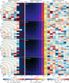 |
Fig. 3 Cylindrically averaged (2D) feed group pseudo-cross-spectra. Columns show, from left to right, the full spectra, the corresponding 1σ uncertainty, and the ratio between the two. Rows show, from top to bottom, Fields 1, 2, 3, and all three combined. The approximate angular scale, assuming the central COMAP redshift at z = 2.9, corresponding to each k⊥ is shown as a twin axis on the upper row of plots. Thin green contours indicate the bin edges of the (1D) spherically averaged FGPXS. |
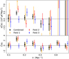 |
Fig. 4 Spherically averaged FGPXS with 1σ uncertainties for Fields 1, 2 and 3 (orange, red and blue respectively) as well as the combination of the three (black) in units μK2 Mpc2 (upper panel) and in units of the 1σ power spectrum uncertainties (lower panel). The data points have been slightly offset from their true k-position to increase readability (see Table B.1 for an overview over bin centers, FGPXS values, and uncertainties). |
5.3 Comparison to COMAP Early Science and COPSS
Having computed the spherically and field-averaged FGPXS from the data we can compare it to the previous COMAP release as well as the CO Power Spectrum Survey (COPSS), the only other comparable CO(1–0) LIM survey in the literature with published data (Keating et al. 2016; Kovetz et al. 2017, 2019; Bernal & Kovetz 2022). This is illustrated in Fig. 5 where the field-averaged FGPXS is plotted together with the COMAP ES constant-elevation-scan FPXS of Ihle et al. (2022) and the individual COPSS data points from Keating et al. (2016).
The first thing we notice when considering Fig. 5 is the dramatic reduction in the uncertainty of the current measurement compared to that from our ES phase (Ihle et al. 2022). Compared to the Ihle et al. (2022) FPXS the current level of sensitivity has increased by a factor ~6–8 across our six most sensitive bins at 0.09 Mpc−1 < k < 0.73 Mpc−1. This illustrates the significant increase in the effective data volume by around a factor of eight. Even though the low-level data selection procedure detailed by Lunde et al. (2024) is somewhat more strict than the one in COMAP ES (Foss et al. 2022; Ihle et al. 2022), this is more than compensated by the lack of data cuts in the power spectrum domain, resulting in a significant increase in sensitivity overall. In other words, we have demonstrated that uncertainties in the power spectra integrate down in accordance with expectations for noise-dominated data.
The two highest k-bins have somewhat larger errors in the current result compared to the COMAP ES spectrum. This is due to a combination of the analytical beam transfer function now applied and a stricter 2D k-space mask. The beam transfer function now applied is somewhat more strict than the numerically computed one of Ihle et al. (2022) on scales closer to the Nyquist limit in the angular direction. Additionally, to avoid problems with aliasing we have masked the outer-most bins in both k∥ and k⊥. As a result, the outer-most 1D k-bins contain a lower number of samples than they would have for the same 1D bins of Ihle et al. (2022).
The COPSS power spectrum estimate (Keating et al. 2016) primarily covers scales smaller than COMAP, but the two experiments overlap at 0.3 Mpc−1 ≲ k ≲ 1.0 Mpc−1, where they are largely consistent with each other. The only noteworthy disagreement between COPSS and the field-combined FGPXS is a mild ~2.5σ tension in terms of the combined error between the two power spectrum estimates at k ~ 0.6 Mpc−1. As we can see from Fig. 5 this point of mild tension coincides with one of the two COPSS points in which they reported a 2.5σ excess above zero.
Albeit with large uncertainties, we see that compared to COPSS and COMAP ES the updated COMAP data points cluster significantly closer to, and are consistent with, the two brightest models that were not already excluded in ES (Chung et al. 2022), namely the COMAP fiducial model3 and the LiKeating model of Keating et al. (2020). For more discussion of the consistency of COPSS with the current COMAP result, including modeling implications, we refer the interested reader to Chung et al. (2024a).
When comparing the power spectrum sensitivity of COMAP to that of COPSS, we must take into account the smaller k-bins in the COPSS analysis. Although the two experiments have a certain region of overlap in k-space, the different bin sizes of COPSS and COMAP result in a different intrinsic within-bin variance. To mitigate this effect we can define the normalized sensitivity ![Mathematical equation: $\[\xi_{k}=\sigma_{k} \sqrt{\Delta V_{k}}\]$](/articles/aa/full_html/2024/11/aa51123-24/aa51123-24-eq52.png) , where ΔVk is the volume of a spherical k-shell defined by the bin k in k-space. Two bins with the same value for ξk would have the same sensitivity, σk, if they were binned to a standardized bin size. In other words, ξk traces the underlying continuous sensitivity of each experiment and k-scale, and as a result, the normalized sensitivity across k-bins and surveys becomes comparable. We illustrate the normalized sensitivity, ξk, in Fig. 6 for all data points shown in Fig. 5. The figure nicely illustrates the scales to which COMAP and COPSS are most sensitive. We see that COMAP is most sensitive on large scales at 0.1 Mpc−1 < k < 0.3 Mpc−1, while COPSS is most sensitive on small scales, 0.5 Mpc−1 < k < 1.0 Mpc−1, where the COMAP beam starts to dominate. However, the current FGPXS result has a peak sensitivity increase of around a factor of eight and ten compared to COMAP ES and COPSS respectively (see Table A.1 for a detailed list of exact normalized sensitivity improvements). This improvement in relative sensitivity compared to COPSS and COMAP ES is expected to increase further as the COMAP instrument gathers more data, and illustrates our ability to remove systematic effects to below the noise level and integrate the noise of the incoming data. In fact, as COPSS to-date remains the only comparable CO(1–0) LIM experiment with published data, COMAP currently provides the most sensitive CO(1–0) LIM constraints in the field.
, where ΔVk is the volume of a spherical k-shell defined by the bin k in k-space. Two bins with the same value for ξk would have the same sensitivity, σk, if they were binned to a standardized bin size. In other words, ξk traces the underlying continuous sensitivity of each experiment and k-scale, and as a result, the normalized sensitivity across k-bins and surveys becomes comparable. We illustrate the normalized sensitivity, ξk, in Fig. 6 for all data points shown in Fig. 5. The figure nicely illustrates the scales to which COMAP and COPSS are most sensitive. We see that COMAP is most sensitive on large scales at 0.1 Mpc−1 < k < 0.3 Mpc−1, while COPSS is most sensitive on small scales, 0.5 Mpc−1 < k < 1.0 Mpc−1, where the COMAP beam starts to dominate. However, the current FGPXS result has a peak sensitivity increase of around a factor of eight and ten compared to COMAP ES and COPSS respectively (see Table A.1 for a detailed list of exact normalized sensitivity improvements). This improvement in relative sensitivity compared to COPSS and COMAP ES is expected to increase further as the COMAP instrument gathers more data, and illustrates our ability to remove systematic effects to below the noise level and integrate the noise of the incoming data. In fact, as COPSS to-date remains the only comparable CO(1–0) LIM experiment with published data, COMAP currently provides the most sensitive CO(1–0) LIM constraints in the field.
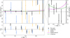 |
Fig. 5 Detailed overview of our field-averaged FGPXS, as well as other datasets and some selected models from the literature. Upper panel: spherically averaged FGPXS with 1σ uncertainties for the field-combined data presented in this paper (black), the COMAP ES field-averaged FPXS (blue; Ihle et al. 2022), and the COPSS power spectrum (orange; Keating et al. 2016). Lower panel: Corresponding power spectra divided by their respective 1σ uncertainty. Inset: zoom-in of the COMAP data points and two comparable models from the literature, namely the fiducial second season COMAP model (Chung et al. 2022) and the Li-Keating model Li et al. (2016); Keating et al. (2020) model. None of the models includes any line-broadening discussed by Chung et al. (2021). Our data points and those of COMAP ES have been slightly offset from their true k-position to increase readability (see Table B.1 for an overview over bin centers, FGPXS values and uncertainties). |
5.4 Upper limits on the power spectrum
Given the factors of, respectively, eight and ten times the sensitivity of our power spectrum result compared to the COMAP ES and COPSS data, it is interesting to consider the upper limits (UL) at 95% confidence on a non-zero CO(1–0) power spectrum that can be derived from the data points. These are shown in Fig. 7 for the spherically and field-averaged COMAP FGPXS, the COMAP ES (Ihle et al. 2022) data points as well as the COPSS (Keating et al. 2016) power spectrum estimate. As we are at the level of sensitivity where it becomes more informative to look at the ULs per k-bin we only consider the ULs derived per k-bin in this work. We show only bin-wise derived ULs from the COMAP ES (Ihle et al. 2022) and COPSS (Keating et al. 2016) data to facilitate a direct comparison to our result. All ULs are computed under the assumption that the astrophysical CO signal must be positive. For comparison, two of the closest models from the literature are included in the plot; the COMAP fiducial model from Chung et al. (2022) and the Li-Keating model – a version of the Li et al. (2016) model from Keating et al. (2020). While the 0.12 Mpc−1 < k < 0.18 Mpc−1 FGPXS bin has a 2.7σ excess above zero, we still present it as a 95% upper limit in Fig. 7 as we do not consider the excess statistically significant.
As in Fig. 6, the ULs we present in Fig. 7 reflect k-regions in which each survey is most sensitive. The 95% ULs of this work and those derived from COMAP ES (Ihle et al. 2022) are most constraining in the six most sensitive COMAP bins at 0.09 Mpc−1 < k < 0.73 Mpc−1. Meanwhile the COPSS Keating et al. (2016) ULs are at their lowest around 0.7 Mpc−1 < k < 1.6 Mpc−1, beyond where the COMAP beam and voxel window dominate and blow up the noise. Compared to COMAP ES, we see a significant improvement in the current ULs per k-bin. Specifically, each of our six most sensitive k-bins can individually constrain k PCO(k) < 2400–4900 μK2 Mpc2 at 95% confidence. The maximum improvement between the two COMAP releases is around a factor 9 in the k ~ 0.4 Mpc−1 bin. The UL estimates are sensitive to both the uncertainty of a data point and its value. As the field-averaged FGPXS in the k ~ 0.4 Mpc−1 bin is around −1.5σ below zero the resulting UL becomes the deepest even though according to Fig. 6 it is not the most sensitive k-bin.
When comparing COPSS to COMAP in Fig. 7 we see that where COMAP and COPSS have overlapping areas of high sensitivity, at k < 0.8 Mpc−1, our 95% ULs are significantly lower than those derived from the COPSS data points. This reflects the increased sensitivity of the COMAP FGPXS estimate already observed in Fig. 6. While none of the updated 95% ULs are touching any of the two included models, a significantly larger region of the power spectrum space is excluded compared to only using the COPSS and COMAP ES limits, and our 95% ULs are starting to encroach on the models that are not already excluded, including the fiducial model (Chung et al. 2022). Given our demonstrated ability to control systematic effects, and the constraints already achieved, detection of a CO power spectrum close to the fiducial model is within reach with further observations.
To conclude the discussion of the power spectrum results, the current COMAP power spectrum is the state-of-the-art CO LIM power spectrum dataset with around an order of magnitude more sensitivity and comparatively lower ULs at 95% confidence than COPSS and COMAPES, the only comparable CO(1–0) line intensity mapping datasets in the literature. The presented power spectrum data points and resulting 95% ULs further exclude a significant portion of the parameter space of possible CO models and provide the current best direct 3D constraints on the CO(1–0) power spectrum in the literature (Kovetz et al. 2017, 2019; Bernal & Kovetz 2022).
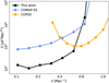 |
Fig. 6 Comparison of volume-normalized sensitivity, ξk, for the new COMAP FGPXS (black); the previous COMAP ES FPXS (blue; Ihle et al. 2022), and COPSS (orange; Keating et al. 2016). The deepest COMAP k-bin is roughly an order of magnitude more sensitive than the deepest COMAP ES and COPSS bins; for tabulated values, see Table A.1. |
6 Null test results
As was described in Sect. 3, we performed a set of null tests by computing the average cross-elevation FGPXS of a set of difference maps. All null tests were performed with the same pipeline and data selection as the power spectrum data shown in Sect. 5. The differencing variables chosen for the null tests were selected to test for correlations owing to a variety of potential systematic effects, for example, environmental effects like weather, sidelobe pickup, and pipeline diagnostics. In Table C.2 we show an overview of the selected null variables.
In total, 312 effective null tests were performed: 26 null test variables across three fields, cylindrical- and spherical-averaged FGPXS as well as separate tests for fast and slow azimuth data respectively. All of these can have different associated systematic effects. For instance, given that the telescope’s scanning speed was changed to a lower azimuthal speed in May 2022, the fast and slow azimuth data (May 2022–November 2023) may have very different mechanical vibrations that could cause spurious patterns in the maps (see Lunde et al. 2024, for examples).
For each of the effective null tests, we calculate corresponding χ2 PTEs, as is described in Sect. 3. We provide a detailed list of these in Appendix C (see Table C.1).
Of the 312 null tests that we performed, the two lowest PTEs were found to be ~0.6%, which amounts to a random binomial probability of 27%. Two of the null test χ2-values were slightly outside the RND simulated χ2-distribution and we therefore only have a lower limit of 99.5% on their PTEs (because the numerical resolution of the simulation-based approach is 1/183 ≈ 0.5%); this could be improved somewhat by using more RND realizations.
The PTEs are expected to follow a uniform distribution. As a consistency check, we therefore consider the PTE distributions of the performed null tests. In Fig. 8 we show the combined PTE distribution for all separately performed null tests (the corresponding distributions for each separately performed category of null tests can be seen in Fig. C.1). To further gauge the uniformity of the histograms a Kolmogorov-Smirnov (KS) test was performed to see if the null test χ2 PTEs were consistent with the null hypothesis of being drawn from a uniform distribution. The KS-test PTE-values are found in Table 2 (and also in the bottom row of Table C.1 of null test χ2 PTEs in Appendix C). The lowest KS-test PTE of 5.5%, corresponds to a binomial probability of around 35% for the 12 performed KS tests. The maximum KS-test PTE is around 79%, and the uniformity of the entire set of PTEs is at the 58.7% level.
We can therefore conclude that all the null tests and PTE uniformity tests have been passed and are consistent with the expected instrumental noise. As we do not claim any detection at this stage, the number and type of null tests performed are more than enough to ensure a sufficient data quality for our upper limits.
7 Conclusion
We have presented updated constraints on the cosmological CO(1–0) power spectrum at 2.4 < z < 3.4, derived from the latest COMAP observations. These measurements are based on a novel mean-averaged feed group pseudo-cross-power spectrum (FGPXS) estimator that is a slight modification of the feedfeed pseudo-cross-power spectrum (FPXS) estimator used in the COMAP ES analysis (Ihle et al. 2022). The difference between these two estimators is that while the previous estimator evaluated cross-correlations between any two detector feeds, the new estimator evaluates cross-correlations between groups of feeds defined by common first downconversion (DCM1) local oscillators. The motivation for this is that feeds in these groups share some common instrumental systematic effects, and the new estimator is therefore more robust against such effects.
Quantitatively, all power spectrum bins were consistent with zero up to ~2σ, except for k ~ 0.15 Mpc−1, which showed a 2–3σ excess in Fields 1 and 2; averaging over all three fields yields an excess of 2.7σ. Despite this single-bin excess, the total PTEs with respect to a zero-signal model are 33.2%, 19.5% and 82.7% for Fields 1–3, respectively, and 34% when combining the data across fields. The resulting FGPXS spectrum derived from the latest COMAP data is thus statistically consistent with instrumental noise, and a detailed suite of null tests shows no signs of residual systematic effects. At the same time, the slight excess at k ~ 0.15 Mpc−1 is noteworthy; it could just be a regular noise fluctuation or the signature of some yet-to-be-discovered systematic effect. However, it could also be a small first hint of true cosmological CO fluctuations. More data are needed to determine its true nature.
Comparing with previous results, we find that the new COMAP power constraints are almost an order of magnitude stronger than the previous ES results (Ihle et al. 2022). In addition, when considering the power spectrum data points alone, the COPSS power spectrum (Keating et al. 2016) was found to be mostly consistent with the COMAP FGPXS, with only a mild ~2.5σ tension in one of the bins. The volume-normalized sensitivity of the COMAP FGPXS was found to be around ten times that of the COPSS power spectrum estimate when comparing the respective most sensitive bins of the two experiments.
We developed a null test framework involving the difference between half-data maps that are split under variables believed to be associated with systematic effects. With the 26 split variables, three fields, the cylindrically and spherically averaged FGPXS as well as the fast- and slow-moving scans a total of 312 effective null tests were performed. Of these all passed within the expected instrumental uncertainties, ensuring the quality of our final data products.
To conclude, our power spectrum estimates and the resulting 95% upper limits provide the most sensitive constraints on cosmic CO emission at z ~ 2–3 published to date and significantly reduce the allowed parameter space of possible CO emission models, the implications of which we explore further in the companion work of Chung et al. (2024a). These results are a strong demonstration of COMAP’s powerful capabilities and performance in terms of systematic effect mitigation, and the filtered data are still dominated by white noise even after three years of integration. Regular operations are still ongoing, and the data currently being gathered will put further pressure on possible CO emission models.
 |
Fig. 7 Comparison of upper 95% confidence limits (ULs) on the CO power spectrum as derived from the new COMAP dataset (black), the COMAP ES analysis (blue; Ihle et al. 2022), and from COPSS (orange; Keating et al. 2016). The corresponding data points for each bin are shown in Fig. 5, and all ULs are derived using a positivity prior. The theoretical model predictions indicated by green and purple lines are the same as in Fig. 5. We note that because the data point of the FGPXS and COMAP ES centered at k = 1.27 Mpc−1 in Figs. 4 and 5 have large uncertainties the corresponding 95% UL are outside y-range of the figure. |
Kolmogorov–Smirnov uniformity test PTEs on the null test χ2 PTEs.
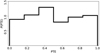 |
Fig. 8 Normalized distribution, P(PTE), of χ2 PTEs for all null tests performed on Fields 1–3 combined. The PTE values corresponding to this histogram are found in Table C.1. The Kolmogorov-Smirnov (KS) uniformity test on the samples contained in the illustrated distribution was found to yield a KS PTE of 58.7% (see Table 2). |
Acknowledgements
We acknowledge support from the Research Council of Norway through grants 251328 and 274990, and from the European Research Council (ERC) under the Horizon 2020 Research and Innovation Program (Grant agreement No. 772253 bits2cosmology and 819478 Cosmoglobe). This material is based upon work supported by the National Science Foundation under Grant Nos. 1517108, 1517288, 1517598, 1518282, 1910999, and 2206834, as well as by the Keck Institute for Space Studies under “The First Billion Years: A Technical Development Program for Spectral Line Observations”. Parts of the work were carried out at the Jet Propulsion Laboratory, California Institute of Technology, under a contract with the National Aeronautics and Space Administration. PCB is supported by the James Arthur Postdoctoral Fellowship HP acknowledges support from the Swiss National Science Foundation via Ambizione Grant PZ00P2_179934. JK acknowledges support from a Robert A. Millikan Fellowship while at Caltech. DC is supported by a CITA/Dunlap Institute postdoctoral fellowship. The Dunlap Institute is funded through an endowment established by the David Dunlap family and the University of Toronto. Research in Canada is supported by NSERC and CIFAR. SEH acknowledges funding from an STFC Consolidated Grant (ST/P000649/1) and a UKSA grant (ST/Y005945/1) funding LiteBIRD foreground activities. JG acknowledges support from the Keck Institute for Space Science, NSF AST-1517108, and University of Miami, and Hugh Medrano for assistance with cryostat design. This work was supported by the National Research Foundation of Korea(NRF) grant funded by the Korean government(MSIT) (RS-2024-00340759). NOS and JGSL extend a great thanks to Sigurd K. Næss for all the fruitful discussions in the office, and while biking through nature, during the last three years. This work was first presented at the Line Intensity Mapping 2024 conference held in Urbana, Illinois; we thank the organizers for their hospitality and the participants for useful discussions. Software acknowledgments. Matplotlib for plotting (Hunter 2007); NumPy (Harris et al. 2020) and SciPy (Virtanen et al. 2020) for efficient numerics and array handling in Python; Astropy a community-made core Python package for astronomy (Astropy Collaboration 2013, 2018, 2022); Multi-node parallelization with MPI for Python (Dalcín et al. 2005, 2008; Dalcin et al. 2011; Dalcin & Fang 2021); Pixell (https://github.com/simonsobs/pixell) for handling sky maps in rectangular pixelization.
Appendix A Normalized CO power spectrum sensitivity
Table A.1 provides a comparison of the volume-normalized CO power spectrum sensitivity for the new COMAP dataset with those power spectra derived from COMAP ES and COPSS; these are visualized in Fig. 6. The volume-normalized sensitivity is defined as
![Mathematical equation: $\[\xi_{k}=\sigma_{k} \sqrt{\Delta V_{k}},\]$](/articles/aa/full_html/2024/11/aa51123-24/aa51123-24-eq53.png) (A.1)
(A.1)
where σk is the uncertainty of a spherically averaged power spectrum bin k with shell volume ΔVk. This definition eliminates the effect of within-bin variance at each k-bin and provides a volume-independent measure that may be used to compare sensitivities between non-overlapping power spectrum bins and surveys. We see that the current COMAP power spectrum constraints reach a maximum sensitivity of one order of magnitude higher than the most sensitive COPSS (Keating et al. 2016) and COMAP ES (Ihle et al. 2022) bins. In addition, it is important to note that the regimes of maximum sensitivity differ between COMAP and COPSS, and this is due to their different instrumental designs and effective angular resolutions; COMAP is more sensitive in the large-scale clustering regime, while COPSS is more sensitive in the small-scale shot-noise regime.
Normalized sensitivity in each COMAP and COPSS bin.
Appendix B Power spectrum data point values
For the interested reader, we provide a list of power spectrum values and uncertainties, ![Mathematical equation: $\[k \tilde{C}(k)\]$](/articles/aa/full_html/2024/11/aa51123-24/aa51123-24-eq56.png) and
and ![Mathematical equation: $\[k \sigma_{\tilde{C}(k)}\]$](/articles/aa/full_html/2024/11/aa51123-24/aa51123-24-eq57.png) respectively, of the spherically and field-averaged FGPXS data points seen in Fig. 5. These can be found in Table B.1.
respectively, of the spherically and field-averaged FGPXS data points seen in Fig. 5. These can be found in Table B.1.
Overview of FGPXS bin values and uncertainties.
Appendix C Null test probabilities-to-exceed
In the following, we present a summary of the χ2 PTEs for each of our effective 312 null tests performed. The PTEs are found in Table C.1 and each null variable, and the corresponding acronyms are explained in detail in Table C.2.
Table C.1 is structured as follows: each row shows a different null variable in which the data was split in two, such as ambient temperature (ambt) or right- and left-moving azimuth sweeps (azdr). The columns are grouped into a hierarchical structure, as we performed null tests separately on spherically and cylindrically averaged FGPXS, for each field (Fields 1–3) as well as for data that were gathered before and after May 2022 when the scanning speed of the telescope was reduced. That is, because the fast- and slow-moving azimuth scans may have different associated systematic effects from, for example, mechanical vibrations in the telescope.
We present the distributions of PTEs of each separately performed null test in Fig. C.1 (see Fig. 8 in Sect. 6 for distribution of all null test PTEs considered jointly). As the distribution of PTEs is expected to be uniform we also performed a Kolmogorov-Smirnov (KS) test to find how probable it is that the PTE samples are drawn from a uniform distribution. These are shown for each separate null test category in the very last row of Table C.1 (and also in Table 2 in Sect. 6). For a discussion on the null test results see Sect. 6.
Detailed overview of null test χ2 PTEs.
Detailed overview and explanation of null test variables.
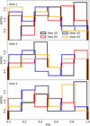 |
Fig. C.1 Normalized distribution, P(PTE), of χ2 PTEs separately for all null tests performed on Field 1-3. The PTE values corresponding to this histogram are found in Table C.1. The Kolmogorov-Smirnov (KS) uniformity test results for the χ2-samples of each of the separate PTE distributions can be found in Table 2 or the bottom row of Table C.1. The individual histograms are slightly offset w.r.t. each other for increased readability. |
Appendix D A simple end-to-end signal injection test
The same type of simulations used to estimate the filter transfer function (see Sect. 4) can also be used to perform a rudimentary end-to-end signal injection test to confirm the detectability of signal given our transfer function estimate. The signal injection pipeline is explained in more detail in Sect. 6.1 of Lunde et al. (2024), and we here limit the scope to the application thereof.
As the signal and noise in the raw data are affected by both the low-level analysis and instrumental effects described by Lunde et al. (2024), an important question to answer is whether we would be able to reconstruct the amplitude of an amplified CO signal within the estimated uncertainties using the earlier described FGPXS method. For instance, we know that several of the PCA filters in the low-level pipeline detailed by Lunde et al. (2024) can in principle act non-linearly if the CO S/N becomes too high. One therefore has to verify that the filters remove equal amounts of signal at any given k-mode of the map in the filter transfer function estimation and for the actual signal estimation from the data. Otherwise, the final signal estimate computed obtained from the data would be biased.
We generate mock signal maps to use in this injection mechanism by applying the fiducial halo model to dark matter halos simulated with the peak-patch technique (Bond & Myers 1996; Stein et al. 2019). Furthermore, we use a raw COMAP data volume corresponding to all the fast-moving azimuth scans of Field 3. This roughly corresponds to the largest independently filtered data volume or, in other words, the highest possible CO S/N. We then boost the injected signal by a factor of three before injecting it into the raw time stream to ensure the signal is detectable above the instrumental noise. Subsequently, the TOD are filtered and binned into maps using the pipeline described by Lunde et al. (2024), before we compute the FGPXS signal estimate to see whether the injected signal was successfully recovered. We note that only one signal realization is used because these high-realism mocks are expensive to produce. However, the test still functions as a simple qualitative “sanity check” that the pipeline works as intended. Future work will expand on this modest check by including further signal realizations and COMAP fields.
The resulting mock FGPXS data points as well as the auto-power spectrum of the input simulation can be seen in Fig. D.1. We can clearly see a high-significance excess that appears consistent with the power spectrum of the input signal within the estimated error bars (which are estimated using the RND methodology described in Sec. 2.3). The excess is large enough to place the computed χ2-value of the mock data far outside the computed RND χ2-distribution. Therefore, to assign a quantitative value to the significance of this mock detection, we instead use the simplified assumptions of approximately Gaussian uncertainties. When doing so, we obtain an estimated ≈ 6σ detection of non-zero power. Meanwhile, testing against the input signal we get a 1.5σ significance away from the model, meaning we recover the input signal within at most mild tension.
This exercise demonstrates that we can recover the input signal within the experimental errors, indicating that our pipeline, the full transfer function, and error bar estimation work as expected.
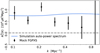 |
Fig. D.1 Example of the spherically averaged FGPXS (black points) resulting from injecting a mock CO signal realization (blue input power spectrum) of the (line-broadened) COMAP fiducial model (Chung et al. 2021, 2022) with a boost factor of three into all fast-moving azimuth data of Field 3. |
References
- Astropy Collaboration (Robitaille, T. P., et al.) 2013, A&A, 558, A33 [NASA ADS] [CrossRef] [EDP Sciences] [Google Scholar]
- Astropy Collaboration (Price-Whelan, A. M., et al.) 2018, AJ, 156, 123 [Google Scholar]
- Astropy Collaboration (Price-Whelan, A. M., et al.) 2022, ApJ, 935, 167 [NASA ADS] [CrossRef] [Google Scholar]
- Battye, R. A., Davies, R. D., & Weller, J. 2004, MNRAS, 355, 1339 [NASA ADS] [CrossRef] [Google Scholar]
- Bernal, J. L., & Kovetz, E. D. 2022, A&A Rev., 30, 5 [NASA ADS] [CrossRef] [Google Scholar]
- Bond, J. R., & Myers, S. T. 1996, ApJS, 103, 1 [NASA ADS] [CrossRef] [Google Scholar]
- Breysse, P. C., Kovetz, E. D., Behroozi, P. S., Dai, L., & Kamionkowski, M. 2017, MNRAS, 467, 2996 [NASA ADS] [Google Scholar]
- Breysse, P. C., Chung, D. T., Cleary, K. A., et al. 2022, ApJ, 933, 188 [NASA ADS] [CrossRef] [Google Scholar]
- Breysse, P. C., Chung, D. T., & Ihle, H. T. 2023, MNRAS, 525, 1824 [CrossRef] [Google Scholar]
- Chung, D. T., Breysse, P. C., Ihle, H. T., et al. 2021, ApJ, 923, 188 [NASA ADS] [CrossRef] [Google Scholar]
- Chung, D. T., Breysse, P. C., Cleary, K. A., et al. 2022, ApJ, 933, 186 [NASA ADS] [CrossRef] [Google Scholar]
- Chung, D. T., Bangari, I., Breysse, P. C., et al. 2023, MNRAS, 520, 5305 [NASA ADS] [CrossRef] [Google Scholar]
- Chung, D. T., Breysse, P. C., Cleary, K. A., et al. 2024a, A&A, 691, A337 (Paper III) [NASA ADS] [CrossRef] [EDP Sciences] [Google Scholar]
- Chung, D. T., Chluba, J., & Breysse, P. C. 2024b, Phys. Rev. D, 110, 023513 [NASA ADS] [CrossRef] [Google Scholar]
- Cleary, K. A., Borowska, J., Breysse, P. C., et al. 2022, ApJ, 933, 182 [NASA ADS] [CrossRef] [Google Scholar]
- Dalcin, L., & Fang, Y.-L. L. 2021, Comput. Sci. Eng., 23, 47 [NASA ADS] [CrossRef] [Google Scholar]
- Dalcín, L., Paz, R., & Storti, M. 2005, J. Parallel Distrib. Comput., 65, 1108 [CrossRef] [Google Scholar]
- Dalcín, L., Paz, R., Storti, M., & D’Elía, J. 2008, J. Parallel Distrib. Comput., 68, 655 [CrossRef] [Google Scholar]
- Dalcin, L. D., Paz, R. R., Kler, P. A., & Cosimo, A. 2011, Adv. Water Resour., 34, 1124 [NASA ADS] [CrossRef] [Google Scholar]
- Dunne, D. A., Cleary, K. A., Breysse, P. C., et al. 2024, ApJ, 965, 7 [NASA ADS] [CrossRef] [Google Scholar]
- Foss, M. K., Ihle, H. T., Borowska, J., et al. 2022, ApJ, 933, 184 [NASA ADS] [CrossRef] [Google Scholar]
- Gaunt, R. E. 2019, Statistica Neerlandica, 73, 176 [CrossRef] [Google Scholar]
- Harris, C. R., Millman, K. J., van der Walt, S. J., et al. 2020, Nature, 585, 357 [NASA ADS] [CrossRef] [Google Scholar]
- Hinshaw, G., Larson, D., Komatsu, E., et al. 2013, ApJS, 208, 19 [Google Scholar]
- Hivon, E., Górski, K. M., Netterfield, C. B., et al. 2002, ApJ, 567, 2 [NASA ADS] [CrossRef] [Google Scholar]
- Hunter, J. D. 2007, Comput. Sci. Eng., 9, 90 [NASA ADS] [CrossRef] [Google Scholar]
- Ihle, H. T., Chung, D., Stein, G., et al. 2019, ApJ, 871, 75 [NASA ADS] [CrossRef] [Google Scholar]
- Ihle, H. T., Borowska, J., Cleary, K. A., et al. 2022, ApJ, 933, 185 [NASA ADS] [CrossRef] [Google Scholar]
- Keating, G. K., Marrone, D. P., Bower, G. C., et al. 2016, ApJ, 830, 34 [NASA ADS] [CrossRef] [Google Scholar]
- Keating, G. K., Marrone, D. P., Bower, G. C., & Keenan, R. P. 2020, ApJ, 901, 141 [NASA ADS] [CrossRef] [Google Scholar]
- Kovetz, E. D., Viero, M. P., Lidz, A., et al. 2017, arXiv e-prints [arXiv:1709.09066] [Google Scholar]
- Kovetz, E., Breysse, P. C., Lidz, A., et al. 2019, BAAS, 51, 101 [NASA ADS] [Google Scholar]
- Lamb, J. W., Cleary, K. A., Woody, D. P., et al. 2022, ApJ, 933, 183 [NASA ADS] [CrossRef] [Google Scholar]
- Leung, J. S. Y., Hartley, J., Nagy, J. M., et al. 2022, ApJ, 928, 109 [NASA ADS] [CrossRef] [Google Scholar]
- Li, T. Y., Wechsler, R. H., Devaraj, K., & Church, S. E. 2016, ApJ, 817, 169 [NASA ADS] [CrossRef] [Google Scholar]
- Loeb, A., & Wyithe, J. S. B. 2008, Phys. Rev. Lett., 100, 161301 [NASA ADS] [CrossRef] [Google Scholar]
- Lunde, J. G. S., Stutzer, N. O., Breysse, P. C., et al. 2024, A&A, 691, A335 (Paper I) [NASA ADS] [CrossRef] [EDP Sciences] [Google Scholar]
- Madau, P., & Dickinson, M. 2014, ARA&A, 52, 415 [Google Scholar]
- Madau, P., Meiksin, A., & Rees, M. J. 1997, ApJ, 475, 429 [NASA ADS] [CrossRef] [Google Scholar]
- Nadarajah, S., & Pogány, T. K. 2016, Comp. Rend. Math., 354, 201 [Google Scholar]
- Peterson, J. B., Bandura, K., & Pen, U. L. 2006, arXiv e-print [astro-ph/0606104] [Google Scholar]
- Rennie, T. J., Harper, S. E., Dickinson, C., et al. 2022, ApJ, 933, 187 [NASA ADS] [CrossRef] [Google Scholar]
- Stein, G., Alvarez, M. A., & Bond, J. R. 2019, MNRAS, 483, 2236 [NASA ADS] [CrossRef] [Google Scholar]
- Virtanen, P., Gommers, R., Oliphant, T. E., et al. 2020, Nature Methods, 17, 261 [CrossRef] [Google Scholar]
- Watts, D. J., Addison, G. E., Bennett, C. L., & Weiland, J. L. 2020, ApJ, 889, 130 [NASA ADS] [CrossRef] [Google Scholar]
We note that technically PCO(k) in this notation would include contributions from both cosmic CO and all other astrophysical components with non-trivial frequency structure that are not subtracted out by the low-level data analysis steps, e.g., potential interloper line emission. However, for CO(1–0) at z = 2–3 there are very few, if any, interloper lines, apart from a ~ 10% contamination from CO(2–1) at z = 6–8 (Breysse et al. 2022; Chung et al. 2024b) that could be picked up, and we therefore use a CO-only notation.
We note that this number in practice tends to be a little larger because we exclude auto-combinations between feed(-groups) and these contain the largest fraction of the optimal total auto-spectrum sensitivity due to better overlapping cross-sky maps.
A double power-law model relating halo masses in cosmological simulations to CO luminosities; see specifically “UM+COLDz+COPSS” in Table 1 of Chung et al. (2022) for their fiducial model definition.
All Tables
All Figures
|
Fig. 1 Example grid of possible feed group (FG1–4) and elevation (high and low) split combinations. Combinations with dark and light gray shading, respectively, represent auto-feed group and auto-elevation combinations that are not used in the final averaged FGPXS. The crosscombinations containing examples of a 2D cross-spectrum contribute to the final average FGPXS as neither identical feed groups, nor elevations, are crossed. |
| In the text | |
|
Fig. 2 Full power spectrum transfer function used to account for the signal losses due to the low-level filtering pipeline, the instrumental beam smoothing, and the voxel window of the maps (see Lunde et al. 2024, for details on each individual transfer function). Thin green contours indicate the bin edges of the (1D) spherically averaged FGPXS. |
| In the text | |
|
Fig. 3 Cylindrically averaged (2D) feed group pseudo-cross-spectra. Columns show, from left to right, the full spectra, the corresponding 1σ uncertainty, and the ratio between the two. Rows show, from top to bottom, Fields 1, 2, 3, and all three combined. The approximate angular scale, assuming the central COMAP redshift at z = 2.9, corresponding to each k⊥ is shown as a twin axis on the upper row of plots. Thin green contours indicate the bin edges of the (1D) spherically averaged FGPXS. |
| In the text | |
|
Fig. 4 Spherically averaged FGPXS with 1σ uncertainties for Fields 1, 2 and 3 (orange, red and blue respectively) as well as the combination of the three (black) in units μK2 Mpc2 (upper panel) and in units of the 1σ power spectrum uncertainties (lower panel). The data points have been slightly offset from their true k-position to increase readability (see Table B.1 for an overview over bin centers, FGPXS values, and uncertainties). |
| In the text | |
|
Fig. 5 Detailed overview of our field-averaged FGPXS, as well as other datasets and some selected models from the literature. Upper panel: spherically averaged FGPXS with 1σ uncertainties for the field-combined data presented in this paper (black), the COMAP ES field-averaged FPXS (blue; Ihle et al. 2022), and the COPSS power spectrum (orange; Keating et al. 2016). Lower panel: Corresponding power spectra divided by their respective 1σ uncertainty. Inset: zoom-in of the COMAP data points and two comparable models from the literature, namely the fiducial second season COMAP model (Chung et al. 2022) and the Li-Keating model Li et al. (2016); Keating et al. (2020) model. None of the models includes any line-broadening discussed by Chung et al. (2021). Our data points and those of COMAP ES have been slightly offset from their true k-position to increase readability (see Table B.1 for an overview over bin centers, FGPXS values and uncertainties). |
| In the text | |
|
Fig. 6 Comparison of volume-normalized sensitivity, ξk, for the new COMAP FGPXS (black); the previous COMAP ES FPXS (blue; Ihle et al. 2022), and COPSS (orange; Keating et al. 2016). The deepest COMAP k-bin is roughly an order of magnitude more sensitive than the deepest COMAP ES and COPSS bins; for tabulated values, see Table A.1. |
| In the text | |
|
Fig. 7 Comparison of upper 95% confidence limits (ULs) on the CO power spectrum as derived from the new COMAP dataset (black), the COMAP ES analysis (blue; Ihle et al. 2022), and from COPSS (orange; Keating et al. 2016). The corresponding data points for each bin are shown in Fig. 5, and all ULs are derived using a positivity prior. The theoretical model predictions indicated by green and purple lines are the same as in Fig. 5. We note that because the data point of the FGPXS and COMAP ES centered at k = 1.27 Mpc−1 in Figs. 4 and 5 have large uncertainties the corresponding 95% UL are outside y-range of the figure. |
| In the text | |
|
Fig. 8 Normalized distribution, P(PTE), of χ2 PTEs for all null tests performed on Fields 1–3 combined. The PTE values corresponding to this histogram are found in Table C.1. The Kolmogorov-Smirnov (KS) uniformity test on the samples contained in the illustrated distribution was found to yield a KS PTE of 58.7% (see Table 2). |
| In the text | |
|
Fig. C.1 Normalized distribution, P(PTE), of χ2 PTEs separately for all null tests performed on Field 1-3. The PTE values corresponding to this histogram are found in Table C.1. The Kolmogorov-Smirnov (KS) uniformity test results for the χ2-samples of each of the separate PTE distributions can be found in Table 2 or the bottom row of Table C.1. The individual histograms are slightly offset w.r.t. each other for increased readability. |
| In the text | |
|
Fig. D.1 Example of the spherically averaged FGPXS (black points) resulting from injecting a mock CO signal realization (blue input power spectrum) of the (line-broadened) COMAP fiducial model (Chung et al. 2021, 2022) with a boost factor of three into all fast-moving azimuth data of Field 3. |
| In the text | |
Current usage metrics show cumulative count of Article Views (full-text article views including HTML views, PDF and ePub downloads, according to the available data) and Abstracts Views on Vision4Press platform.
Data correspond to usage on the plateform after 2015. The current usage metrics is available 48-96 hours after online publication and is updated daily on week days.
Initial download of the metrics may take a while.