| Issue |
A&A
Volume 691, November 2024
|
|
|---|---|---|
| Article Number | A337 | |
| Number of page(s) | 14 | |
| Section | Cosmology (including clusters of galaxies) | |
| DOI | https://doi.org/10.1051/0004-6361/202451122 | |
| Published online | 27 November 2024 | |
COMAP Pathfinder – Season 2 results
III. Implications for cosmic molecular gas content at z ~ 3
1
Canadian Institute for Theoretical Astrophysics, University of Toronto,
60 St. George Street,
Toronto,
ON
M5S 3H8,
Canada
2
Dunlap Institute for Astronomy and Astrophysics, University of Toronto,
50 St. George Street,
Toronto,
ON
M5S 3H4,
Canada
3
Department of Astronomy, Cornell University,
Ithaca,
NY
14853,
USA
4
Center for Cosmology and Particle Physics, Department of Physics, New York University,
726 Broadway,
New York,
NY
10003,
USA
5
Department of Physics, Southern Methodist University,
Dallas,
TX
75275,
USA
6
California Institute of Technology,
1200 E. California Blvd.,
Pasadena,
CA
91125,
USA
7
Institute of Theoretical Astrophysics, University of Oslo,
PO Box 1029 Blindern,
0315
Oslo,
Norway
8
Departement de Physique Théorique, Universite de Genève,
24 Quai Ernest-Ansermet,
CH-1211
Genève 4,
Switzerland
9
Department of Physics, University of Toronto,
60 St. George Street,
Toronto,
ON
M5S 1A7,
Canada
10
David A. Dunlap Department of Astronomy, University of Toronto,
50 St. George Street,
Toronto,
ON,
M5S 3H4,
Canada
11
Kavli Institute for Particle Astrophysics and Cosmology & Physics Department, Stanford University,
Stanford,
CA
94305,
USA
12
Jet Propulsion Laboratory, California Institute of Technology,
4800 Oak Grove Drive,
Pasadena,
CA
91109,
USA
13
Department of Physics, University of Miami,
1320 Campo Sano Avenue,
Coral Gables,
FL
33146,
USA
14
Jodrell Bank Centre for Astrophysics, Department of Physics & Astronomy, The University of Manchester,
Oxford Road,
Manchester
M13 9PL,
UK
15
Department of Astronomy, University of Maryland,
College Park,
MD
20742,
USA
16
Owens Valley Radio Observatory, California Institute of Technology,
Big Pine,
CA
93513,
USA
17
Department of Physics, Korea Advanced Institute of Science and Technology (KAIST),
291 Daehak-ro, Yuseong-gu,
Daejeon
34141,
Republic of Korea
18
Brookhaven National Laboratory,
Upton,
NY
11973-5000,
USA
19
Department of Physics and Astronomy, University of British Columbia,
Vancouver,
BC
V6T 1Z1,
Canada
★ Corresponding author; This email address is being protected from spambots. You need JavaScript enabled to view it.
Received:
14
June
2024
Accepted:
23
September
2024
Abstract
The Carbon monOxide Mapping Array Project (COMAP) Pathfinder survey continues to demonstrate the feasibility of line-intensity mapping using high-redshift carbon monoxide (CO) line emission traced at cosmological scales. The latest COMAP Pathfinder power spectrum analysis is based on observations through the end of Season 2, covering the first three years of Pathfinder operations. We use our latest constraints on the CO(1–0) line-intensity power spectrum at z ~ 3 to update corresponding constraints on the cosmological clustering of CO line emission and thus the cosmic molecular gas content at a key epoch of galaxy assembly. We first mirror the COMAP Early Science interpretation, considering how Season 2 results translate to limits on the shot noise power of CO fluctuations and the bias of CO emission as a tracer of the underlying dark matter distribution. The COMAP Season 2 results place the most stringent limits on the CO tracer bias to date, at ⟨T b⟩ < 4.8 μK, which translates to a molecular gas density upper limit of ρH2 < 1.6 × 10⁸ M⊙ Mpc−3 at z ~ 3 given additional model assumptions. These limits narrow the model space significantly compared to previous CO line-intensity mapping results while maintaining consistency with small-volume interferometric surveys of resolved line candidates. The results also express a weak preference for CO emission models used to guide fiducial forecasts from COMAP Early Science, including our data-driven priors. We also consider directly constraining a model of the halo–CO connection, and show qualitative hints of capturing the total contribution of faint CO emitters through the improved sensitivity of COMAP data. With continued observations and matching improvements in analysis, the COMAP Pathfinder remains on track for a detection of cosmological clustering of CO emission.
Key words: galaxies: high-redshift / diffuse radiation / radio lines: galaxies
© The Authors 2024
 Open Access article, published by EDP Sciences, under the terms of the Creative Commons Attribution License (https://creativecommons.org/licenses/by/4.0), which permits unrestricted use, distribution, and reproduction in any medium, provided the original work is properly cited.
This article is published in open access under the Subscribe to Open model. This email address is being protected from spambots. You need JavaScript enabled to view it. to support open access publication.
1 Introduction
Line-intensity mapping (LIM) surveys map the large-scale structure of the Universe in large cosmological volumes, but notthrough discrete resolved tracer sources. Rather, LIM surveys achieve this through unresolved emission in specific spectral lines, including lines associated with different phases of the star-forming interstellar medium (ISM) such as carbon monoxide (CO) and the [C II] line from singly ionized carbon (see Kovetz et al. 2019 and Bernal & Kovetz 2022 for recent reviews). As part of a range of emerging interferometric and single-dish LIM surveys from radio to sub-millimeter wavelengths, the CO Mapping Array Project (COMAP; Cleary et al. 2022) is building a dedicated centimeter-wave LIM program to map the cosmic clustering of emission in the CO(1–0) and CO(2–1) lines from the epochs of galaxy assembly (z ~ 3, just before so-called “cosmic noon”) and reionization (z ~ 7, “cosmic dawn”). COMAP science encompasses both the astrophysics of the assembly of molecular gas at these key epochs of galaxy evolution, and ultimately the cosmological implications of observed high-redshift large-scale structure traced by CO emission.
The first phase of COMAP is the COMAP Pathfinder, a 26–34 GHz spectrometer comprising a single-polarization 19-feed array of coherent receivers on a single 10-meter dish at the Owens Valley Radio Observatory (Lamb et al. 2022). The focus of the Pathfinder survey is on CO(1–0) emission from z ~ 3, or a lookback time of ~11.5 Gyr. Around this “cosmic halfpast eleven”, we survey galaxies assembling towards the “cosmic noon” of peak cosmic star formation activity (Somerville & Davé 2015; Förster Schreiber & Wuyts 2020). Following the Early Science analysis of Foss et al. (2022) and Ihle et al. (2022) based on the first season of observations (Season 1), the Season 2 data analysis by Lunde et al. (2024) and Stutzer et al. (2024) encompasses three years of observations and improved data cleaning methods for almost an order-of-magnitude increase in power spectrum sensitivity.
With such progress continuing to demonstrate the feasibility of CO LIM survey operations and low-level data analysis, we present here the corresponding update on our understanding of CO(1–0) emission at z ~ 3. To better understand high-redshift CO(1–0) emission is to better understand the molecular gas content of the high-redshift universe. Previous studies (as reviewed by, e.g., Carilli & Walter 2013) have established the strong correlation between CO line luminosity and dust-obscured star formation activity across a diversity of low- and high-redshift galaxies, as should be expected for a tracer of cold molecular gas that fuels such star formation activity. Using a LIM approach to surveying CO line emission across large cosmological volumes efficiently maps the luminosity density of this emission across such volumes – integrated across faint and bright galaxies alike – and thus sheds light on the cosmic molecular gas content and thus cosmic star formation history in ways that strongly complement conventional surveys cataloguing individual line emitters or star-forming galaxies (Pavesi et al. 2018; Decarli et al. 2020; Lenkić et al. 2020; Garratt et al. 2021). The Pathfinder survey at “cosmic half-past eleven” is only the first step towards extending our understanding of the history of cosmic gas and star formation towards “cosmic dawn”, but a key step nonetheless in testing our ability to use LIM statistics to derive astrophysical constraints of noteworthy constraining power.
We carry out a high-level analysis of the power spectrum constraints of Stutzer et al. (2024) to answer the following questions:
“How much does the increased data volume improve constraints on the clustering and shot noise power of cosmological CO(1–0) emission at z ~ 3?”
“Can COMAP Season 2 data better constrain the empirical connection between CO emission and the underlying structures of dark matter?”
We structure the paper as follows. In Sect. 2 we outline our methodology for interpretation, including but no longer limited to methods previously used in Chung et al. (2022). We discuss the results of our analysis in Sect. 3, and implications for understanding CO emission and interpreting past and future CO LIM surveys in Sect. 4. We end with our primary conclusions and future outlook in Sect. 5.
We assume a ΛCDM cosmology with parameters Ωm = 0.286, ΩΛ = 0.714, Ωb = 0.047, H0 = 100h km s−1 Mpc−1 with h = 0.7, σ8 = 0.82, and ns = 0.96, to maintain consistency with previous COMAP simulations (starting with Li et al. 2016). Distances carry an implicit h−1 dependence throughout, which propagates through masses (all based on virial halo masses, proportional to h−1) and volume densities (∝ h3). Logarithms are base-10 unless stated otherwise.
2 Methods
The primary target of the COMAP Pathfinder is the power spectrum of spatial-spectral emission after subtraction of continuum emission and systematic effects. Any residual fluctuations should predominantly arise from clustered populations of CO-emitting high-redshift galaxies, meaning that we interpret any constraints on the residual emission as constraints on these CO emitters. In the simplest possible model, the power spectrum as a function of comoving wavenumber k consists of the matter power spectrum Pm(k) scaled by some amplitude Aclust, plus a scale-independent shot noise amplitude Pshot:
![Mathematical equation: $\[P(k)=A_{\text {clust }} P_{m}(k)+P_{\text {shot }}.\]$](/articles/aa/full_html/2024/11/aa51122-24/aa51122-24-eq1.png) (1)
(1)
The matter power spectrum describes the distribution of matter density contrast across comoving space, and evolves with redshift as large-scale structure forms and grows. The spatialspectral fluctuations in CO brightness temperature across cosmological scales trace the clustering of the underlying matter fluctuations with some bias, which informs the clustering amplitude Aclust. In combination with halo models of CO emission that postulate average CO luminosities per halo of collapsed dark matter, constraining Aclust (or related quantities) and Pshot allows us to understand not just the global cosmic abundance of CO, but also the relative contribution of different sizes of halos and thus of galaxies. Estimation of the CO line power spectrum P(k) is thus a key target of COMAP low-level analyses.
The goal of this section is to outline methods for the kind of analyses suitable for the current level of sensitivity achieved by the COMAP dataset. First, Sect. 2.1 reviews the COMAP Season 2 power spectrum results in relation to previous work. Then, Sect. 2.2 reviews a simple two-parameter analysis as carried out by Chung et al. (2022) for COMAP Early Science, constraining the clustering and shot noise amplitudes and only indirectly using halo models to support physical interpretation. Finally, Sect. 2.3 outlines a five-parameter analysis to directly constrain a halo model of CO emission, as carried out by Chung et al. (2022) to derive priors for COMAP Early Science but incorporating COMAP data for the first time.
2.1 Foundational data: COMAP Season 2 power spectrum constraints
The present work made use of the results of Stutzer et al. (2024), which derived updated power spectrum constraints based on COMAP Pathfinder survey data collected across 17500 hours over three fields of 2–3 deg2 each, between its commissioning in May 2019 and the end of the second observing season in November 2023. We also made use of the prior work of the CO Power Spectrum Survey (COPSS; Keating et al. 2016), which performed a pilot CO LIM survey targeting largely the same observing frequencies, but with an interferometric dataset probing smaller scales. The COMAP observations are subject to the effects of instrument and pipeline response, such as filtering, pixelization, and beam smoothing. However, the results as considered in this work correct for these effects by applying the inverse of the estimated power spectrum transfer function per k-bin. We expect mode mixing in COMAP data is still at the level of Ihle et al. (2022) at most, that is to say less than 20% for the comoving wavenumber range of k ≳ 0.1 Mpc−1 that we consider.
Fig. 1 shows these results alongside the range of expectations for the z ~ 3 CO(1–0) emission power spectrum from empirical modeling in the decade leading up to this dataset (Pullen et al. 2013; Li et al. 2016; Padmanabhan 2018; Keating et al. 2020; Chung et al. 2022; Yang et al. 2022). These models either postulate a connection between dark matter halo properties and CO luminosity via intermediate galaxy properties such as the star formation rate (SFR), or directly model the halo–CO connection constrained by observed CO luminosity functions and CO LIM measurements.
Of the models shown in Fig. 1, only the models of Padmanabhan (2018) and Chung et al. (2022) fall into the latter category. Keating et al. (2020) also provide empirical estimates for the clustering and shot noise amplitudes, but this is simply based on decomposing the COPSS measurement of Keating et al. (2016) into clustering and shot noise components, rather than a detailed halo model. In a different context Keating et al. (2020) do provide a halo model, which we term the Li et al. (2016)–Keating et al. (2020) model, varying the Li et al. (2016) model by using the same halo–SFR connection from Behroozi et al. (2013a,b) but replacing the SFR–CO connection (via infrared luminosity) derived from a compilation of local and high-redshift galaxies (Carilli & Walter 2013) with one based on a local sample observed by Kamenetzky et al. (2016).
Even before any detailed analyses, compared to COMAP Season 1 we clearly see an increasing rejection of Model B of Pullen et al. (2013) and of the Padmanabhan (2018) model with CO emission duty cycle fduty = 1. We refer the reader to the Early Science work of Chung et al. (2022) for the implications of excluding these models. As with COMAP Early Science, we exclude these models in the clustering regime, rather than the shot-noise dominated scales surveyed by COPSS. However, the COMAP Season 2 sensitivity is sufficient to exclude these models clearly in individual k-bins of width Δ(log k Mpc) = 0.155, rather than having to rely on a co-added measurement across all k as was necessary in Early Science. For reference, we show in Appendix A the original data points behind these upper limits, in a way that more closely resembles Fig. 4 of Stutzer et al. (2024).
Note also a weak tension against the previous positive COPSS measurement in overlapping k-ranges. The original COPSS analysis of Keating et al. (2016) measured the CO power spectrum at k = 1h Mpc−1 to be P(k) = (3.0 ± 1.3) × 103h−3 μK2 Mpc3, for a best estimate of P(k = 0.7 Mpc1) = 8.7 × 10³ μK2 Mpc3. This is co-added across the entire k-range spanned by COPSS, with the highest sensitivity achieved around k = 0.5h–2h Mpc−1. By contrast, in a single k-bin spanning k = 0.52–0.75 Mpc−1, the present COMAP data places a 95% upper limit of 7.9 × 10³ μK2 Mpc3, lying below the COPSS co-added best estimate. However, the COPSS result is itself only a tentative one at ≈ 2.3σ significance, and so there is no statistically significant discrepancy. COMAP data are also entirely consistent with the estimate of ![Mathematical equation: $\[P_{\text {shot }}=2.0_{-1.2}^{+1.1} \times 10^{3} h^{-3} \mu \mathrm{K}^{2} ~\mathrm{Mpc}^{3}\]$](/articles/aa/full_html/2024/11/aa51122-24/aa51122-24-eq2.png) from the later re-analysis of COPSS data by Keating et al. (2020), which marginalized over the possible contribution to P(k) from clustering. In fact our power spectrum results show a marginal excess at k ≈ 0.15 Mpc−1 that, while well below the upper limit implied by the direct COPSS re-analysis of Keating et al. (2020), does tentatively indicate a preference for models similar to the Li et al. (2016)–Keating et al. (2020) model. The remainder of this work establishes this preference more quantitatively, and consider other implications of these results.
from the later re-analysis of COPSS data by Keating et al. (2020), which marginalized over the possible contribution to P(k) from clustering. In fact our power spectrum results show a marginal excess at k ≈ 0.15 Mpc−1 that, while well below the upper limit implied by the direct COPSS re-analysis of Keating et al. (2020), does tentatively indicate a preference for models similar to the Li et al. (2016)–Keating et al. (2020) model. The remainder of this work establishes this preference more quantitatively, and consider other implications of these results.
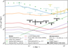 |
Fig. 1 COMAP Season 2 95% upper limits (given P(k) > 0) on the z ~ 3 CO(1–0) power spectrum, with analogous limits from COPSS (Keating et al. 2016) and COMAP Season 1 (Chung et al. 2022). Some k-bins in COPSS and COMAP Season 2 data show marginal excesses, influencing analyses in this work; we thus show 1σ intervals for these bins unlike in Stutzer et al. (2024). We also show predictions based on Chung et al. (2022), Padmanabhan (2018), Pullen et al. (2013), Li et al. (2016), and Yang et al. (2022), plus a variation on the Li et al. (2016) model from Keating et al. (2020), and the Keating et al. (2020) re-analysis of COPSS constraining clustering (triangles) and shot-noise amplitudes (dashed line). |
2.2 Two-parameter analysis: Constraining CO tracer bias and shot noise
The most direct way to analyze the COMAP Season 2 constraints is to decompose the CO power spectrum into clustering and shot noise terms as in Eq. (1), with a fixed cosmological model and no assumptions around detailed astrophysical modeling. The COMAP data then constrain the possible range of values for Aclust and Pshot, which we may then compare to model predictions for these amplitudes for the clustering and shot noise contributions to the power spectrum.
However, physical interpretation requires some amount of guidance from models. For a halo model of CO emission where halos of virial mass Mh emit with CO luminosity L(Mh), we might know the halo mass function dn/dMh describing the differential number density of halos of mass Mh, and the bias bh(Mh) with which the halo number density contrast traces the continuous dark matter density contrast. Then the cosmological fluctuations in CO(1–0) line temperature trace the underlying dark matter fluctuations with a linear scaling of
![Mathematical equation: $\[\langle T b\rangle \propto \int d M_{h} \frac{d n}{d M_{h}} L(M_{h}) b_{h}(M_{h}).\]$](/articles/aa/full_html/2024/11/aa51122-24/aa51122-24-eq3.png) (2)
(2)
This should be understood as a mean line temperature–bias product, with appropriate normalization factors applied to convert luminosity density to brightness temperature. We may also ascribe a dimensionless bias b to CO emission contrast by dividing out the average line temperature or luminosity density:
![Mathematical equation: $\[b=\frac{\int d M_{h}\left(d n / d M_{h}\right) L\left(M_{h}\right) b_{h}\left(M_{h}\right)}{\int d M_{h}\left(d n / d M_{h}\right) L\left(M_{h}\right)}.\]$](/articles/aa/full_html/2024/11/aa51122-24/aa51122-24-eq4.png) (3)
(3)
Furthermore, any halo model of L(Mh) predicts the shot noise, proportional to the second bias- and abundance-weighted moment of the L(Mh) function rather than the first moment:
![Mathematical equation: $\[P_{\text {shot }} \propto \int d M_{h} \frac{d n}{d M_{h}} L^{2}(M_{h}) b_{h}(M_{h}).\]$](/articles/aa/full_html/2024/11/aa51122-24/aa51122-24-eq5.png) (4)
(4)
The quantity Pshot directly describes the shot noise amplitude, but the same is not true of ⟨T b⟩ in relation to the clustering amplitude. In real comoving space we would expect Aclust = ⟨T b⟩2, but redshift-space distortions (RSD) enhance the clustering term as large-scale structure coherently attracts galaxies (Kaiser 1987; Hamilton 1998). In the linear regime of small k, and given that Ωm(z) ≈ 1 at COMAP redshifts,
![Mathematical equation: $\[A_{\text {clust }} \approx\langle T b\rangle^{2}\left(1+\frac{2}{3 b}+\frac{1}{5 b^{2}}\right).\]$](/articles/aa/full_html/2024/11/aa51122-24/aa51122-24-eq6.png) (5)
(5)
Based on prior modeling efforts, we consider b > 2 to be a fairly conservative lower bound on CO tracer bias, as outlined by Chung et al. (2022). This bound on b in turn allows us to bound ⟨T⟩ = ⟨T b⟩ / b based on an upper bound on Aclust.
We considered two variants of a two-parameter analysis of the COMAP data, the same carried out in Chung et al. (2022).
The first variant is a model-agnostic evaluation of the likelihood of different values of Aclust and Pshot given the P(k) data points available from the COPSS results of Keating et al. (2016) and/or from COMAP data through Season 2. We only invoke a conservative limit of b > 2 to obtain an upper bound on ⟨T⟩ from our constraint on Aclust.
The second variant assumes that given values for ⟨T b⟩2 and Pshot, we can expect specific values for b and for an effective line width veff describing the suppression of the high-k CO power spectrum from line broadening (Chung et al. 2021). Exploration of an empirically constrained model space informs fitting functions for b and veff given only ⟨T b⟩2 and Pshot, as provided in Appendix B of Chung et al. (2022), which then enter into calculation of the redshift-space P(k) accounting for RSD and line broadening. We can directly compare this P(k) to our P(k) data to evaluate the likelihood of different values of ⟨T b⟩2 and Pshot. We refer to this variant as the “b- and veff-informed” analysis, versus the first “b- and veff-agnostic” version.
We may then compare likely and unlikely regions of this twoparameter space to model predictions.
2.3 Five-parameter analysis: Directly constraining the halo–CO connection
Neither variant of our two-parameter analysis truly directly constrains the physical picture of CO emission, only a clustering term and a shot noise term. Given a fixed set of power spectrum measurements, the two-parameter analysis broadly projects likelihood contours favouring either high clustering and low shot noise, or low clustering and high shot noise. Yet physical models should impose a strong prior such that clustering and shot noise co-vary, given that the shot noise also tracks with luminosity density, albeit at a higher order – cf. Eq. (4).
Directly modeling and constraining L(Mh) thus has its uses. While dark matter halos are not themselves the direct source of CO emission or indeed any baryonic physics, a halo model of CO emission still serves as a simple way to physically ground interpretation of our CO measurements and introduce priors based on other empirical constraints on the galaxy–halo connection.
2.3.1 Parameterization and derivation of “UM+COLDz” posterior
To model L(Mh), we used the same parameterization and datadriven procedure as in Chung et al. (2022). One of the datasets driving this procedure is provided by the CO Luminosity Density at High-z (COLDz) survey (Pavesi et al. 2018; Riechers et al. 2019), which identified line candidates at z ~ 2.4 through an untargeted interferometric search. In Chung et al. (2022) we also introduced somewhat informative priors based loosely on the work of Behroozi et al. (2019), which devised the UNIVERSEMACHINE (UM) framework for an empirical model of the galaxy–halo connection by connecting halo accretion histories to a minimal model of stellar mass growth. We thus once again combined these “UM” priors with COLDz data and a basic L(Mh) parameterization, just as in Chung et al. (2022).
We assumed a double power law for the linear average L(Mh). In observer units,
![Mathematical equation: $\[\begin{equation*}\frac{L_{\mathrm{CO}}^{\prime}(M_{h})}{\mathrm{K~km} \mathrm{~s}^{-1} ~\mathrm{pc}^{2}}=\frac{C}{\left(M_{h} / M\right)^{A}+\left(M_{h} / M\right)^{B}}.\end{equation*}\]$](/articles/aa/full_html/2024/11/aa51122-24/aa51122-24-eq7.png) (6)
(6)
For CO(1–0),
![Mathematical equation: $\[\begin{equation*}\frac{L_{\mathrm{CO}}(M_{h})}{L_{\odot}}=4.9 \times 10^{-5} \times \frac{L_{\mathrm{CO}}^{\prime}(M_{h})}{\mathrm{K~km} ~\mathrm{s}^{-1} ~\mathrm{pc}^{2}}.\end{equation*}\]$](/articles/aa/full_html/2024/11/aa51122-24/aa51122-24-eq8.png) (7)
(7)
We also modeled stochasticity albeit in a highly simplistic fashion, assuming some level of log-normal scatter σ (in units of dex) about the average relation. We inherit this practice from the common use of log-normal distributions to model intrinsic scatter in, e.g., the halo–SFR connection (e.g.: Behroozi et al. 2013a,b) and the halo–CO connection as modeled for previous early COMAP forecasts (Li et al. 2016).
The somewhat informative “UM” priors for the five free parameters of L(Mh) are as follows:
![Mathematical equation: $\[A =-1.66 \pm 2.33,\]$](/articles/aa/full_html/2024/11/aa51122-24/aa51122-24-eq9.png) (8)
(8)
![Mathematical equation: $\[B = 0.04 \pm 1.26,\]$](/articles/aa/full_html/2024/11/aa51122-24/aa51122-24-eq10.png) (9)
(9)
![Mathematical equation: $\[\log ~C =10.25 \pm 5.29,\]$](/articles/aa/full_html/2024/11/aa51122-24/aa51122-24-eq11.png) (10)
(10)
![Mathematical equation: $\[\log ~\left(M / M_{\odot}\right) =12.41 \pm 1.77.\]$](/articles/aa/full_html/2024/11/aa51122-24/aa51122-24-eq12.png) (11)
(11)
For log-normal scatter, we assumed an initial prior of σ = 0.4 ± 0.2 (dex), taking cues from Li et al. (2016) for the central value and slightly broadening the prior. We review the derivation of priors for all of these parameters in somewhat more detail in Appendix B.
We then narrowed these priors further by matching the luminosity function constraints of the COLDz survey. The matching procedure is similar to that used in Chung et al. (2022). However, that procedure used a snapshot from the Bolshoi–Planck simulation, used by Behroozi et al. (2019) but slightly discrepant against our fiducial cosmology. Here, we used our own peak-patch mocks (Stein et al. 2019) with virial masses matched to the halo mass function of Tinker et al. (2008). We extracted halos from z ∈ (2.35, 2.45) (or χ ∈ (5720.37, 5844.19) Mpc) from these peak-patch mocks, since we are specifically trying to match a luminosity function constraint at z ~ 2.4. We thus obtained 161 independent realizations of a halo catalogue from a 1140 × 1140 × 124 Mpc3 = 0.16 Gpc3 box, comparable to the Bolshoi–Planck snapshot with a box size of (250/0.678) Mpc (or a volume of 0.05 Gpc3). A Markov chain Monte Carlo (MCMC) procedure identifies the posterior (narrowed prior) based on a likelihood calculation in addition to the mildly informative priors outlined above. At each step:
We used the sampled L(Mh) parameters to convert a random peak-patch realization of halo masses into CO luminosities.
We then fit a Schechter function to the resulting CO luminosity function of that randomly chosen peak-patch box.
We calculated the log-likelihood by comparing the Schechter function fit against the COLDz posterior for the Schechter function parameters via a kernel density estimator.
The MCMC used 250 walkers for 4242 steps, and we discarded the first 1000 steps as a burn-in phase. The result is an informed distribution, which we call the “UM+COLDz” posterior, for the five parameters {A, B, C, M, σ} of our L(Mh) model.
2.3.2 Derivation of posteriors incorporating CO LIM data
To derive posteriors based on CO LIM power spectrum measurements, we reran the same MCMC procedure used to derive the “UM+COLDz” distribution with additional contributions to the likelihood from any discrepancy with the CO LIM results. In other words, we introduced additive log-likelihood terms,
![Mathematical equation: $\[\Delta(\log ~\mathcal{L}) \propto-\sum_{k} \frac{[P_{\mathrm{model}}(k)-P_{\text {data}}(k)]^{2}}{\sigma^{2}[P_{\text {data}}(k)]},\]$](/articles/aa/full_html/2024/11/aa51122-24/aa51122-24-eq13.png) (12)
(12)
evaluated against each dataset Pdata(k) with error σ[Pdata(k)] for the model Pmodel(k) drawn at each MCMC step1.
Using our fiducial cosmology and the halo mass function of Tinker et al. (2008), we numerically evaluated closed-form expressions describing the CO power spectrum at z ~ 2.8. We evaluated the above log-likelihood terms against the predicted Pmodel(k) without imposing positivity priors, which would be redundant with the always positive predictions of our P(k) model.
We considered three (combinations of) datasets:
The “UM+COLDz+COPSS” posterior derives from considering only the addition of COPSS data points as shown in Keating et al. (2016).
The “UM+COLDz+COPSS+COMAP S1” posterior derives from considering both COPSS and COMAP Early Science P(k) constraints from Season 1 data.
The “UM+COLDz+COPSS+COMAP S2” posterior derives from considering constraints from both COPSS and the present work on COMAP Pathfinder data through Season 2.
While the MCMC procedure itself evaluates posteriors for {A, B, C, M, σ}, we can use the resulting sampling of parameter space to obtain posterior distributions for derived quantities such as L(Mh), ⟨T⟩, b, and Pshot. In doing so, we can look for how (if at all) the “UM+COLDz+COPSS+COMAP S2” posterior distinguishes itself from posteriors based on only previous data.
3 Results
Having outlined the datasets and methods used in the analyses, we now review the results in relation to previous models and results. We consider outcomes of the two-paramater analysis identifying overall amplitudes for clustering and shot noise power in Sect. 3.1, followed by outcomes of the five-parameter analysis fitting for the L(Mh) relation in Sect. 3.2.
3.1 Two-parameter analysis
We summarize the results of the two-parameter analysis of the COMAP results in Table 1, and show in Fig. 2 the probability distributions when considering only COMAP data up to Season 2 (“COMAP S2” in Table 1). We find a factor of 5 improvement in our ability to constrain Pshot from above with COMAP data alone up to Season 2 compared to COMAP Early Science alone, and a factor of 2 improvement in upper limits for the clustering amplitude. In fact, framing sensitivity to clustering purely in terms of the upper limit achieved downplays our gain. Where the COMAP Early Science analysis effectively gave a maximum a posteriori (MAP) estimate of zero for Aclust and ⟨T b⟩2, Fig. 2 shows that the likelihood distributions peak at positive values of these parameters under COMAP Season 2 constraints.
We also show in Fig. 2 model predictions for Aclust and Pshot, or for ⟨T b⟩2 and Pshot. As expected, all models not shown to be excluded by the COMAP Season 2 data at 95% confidence in Fig. 1 are consistent to within 2σ of the MAP estimate from the COMAP Season 2 likelihood analysis, including the COMAP Early Science fiducial model from Chung et al. (2022). That said, the most favoured model (within 1σ of the MAP estimate) is the Li et al. (2016)–Keating et al. (2020) model used to explain the results of the mm-wave Intensity Mapping Experiment (mmIME; Keating et al. 2020). This finding is consistent between the b- and veff-agnostic and -informed analyses.
The resulting constraints on ⟨T⟩ given b > 2 are also consistent between these analyses to within a few percent. Going forward we quote ⟨T b⟩ < 4.8 μK or ⟨T⟩ < 2.4 μK, consistent with both of our “COMAP S2” standalone analyses as well as both of the “COMAP S2+COPSS” joint analyses as we show in Table 1. As in Chung et al. (2022) we can convert any estimate of ⟨T⟩ into an estimate for cosmic molecular gas density:
![Mathematical equation: $\[\rho_{\mathrm{H} 2}=\alpha_{\mathrm{CO}}\langle T\rangle H(z) /(1+z)^{2}.\]$](/articles/aa/full_html/2024/11/aa51122-24/aa51122-24-eq18.png) (13)
(13)
We show the resulting bounds on ρH2 in Table 1 alongside the original bounds on ⟨T⟩, given αCO = 3.6 M⊙ (K km s−1 pc2)−1 and the Hubble parameter H(z) at the central COMAP redshift of z ~ 2.8. Although some works have advocated for values of αCO (Bolatto et al. 2013; Scoville et al. 2016) higher by as much as a factor of two – and in Sect. C we discuss in more detail what motivates different values of αCO – our chosen value follows the one most commonly used by previous CO line search and line-intensity mapping analyses (e.g.: Riechers et al. 2019; Decarli et al. 2020; Lenkić et al. 2020; Keating et al. 2020), with this value originally identified in three z ~ 1.5 galaxies (Daddi et al. 2010). Our top-line result of ⟨T⟩ < 2.4 μK corresponds to a bound of ρH2 < 1.6 × 10⁸ M⊙ Mpc−3.
When we use COPSS data in combination with COMAP Season 2 data, the results change to favour higher shot noise values as shown in Fig. 3. The constraints on the clustering amplitude, whether phrased as Aclust in a b-/veff-agnostic analysis or ⟨T b⟩2 in a b-/veff-informed analysis, is essentially the same under COMAP Season 2 constraints with or without COPSS data. Note however that in the Early Science analyses of Chung et al. (2022), the COPSS data dominated the constraint on Pshot and weakly favoured a positive value, with the b/veff-agnostic 2D probability distribution between Aclust and Pshot resembling a 2D Gaussian distribution just truncated at the 2σ contour by the Pshot = 0 boundary. This is no longer the case, with the corresponding distribution in the upper portion of Fig. 3 resembling a 2D Gaussian distribution truncated inside the 1σ contour.
What greater allowance remains for higher Pshot values still comes from the way in which the b-/veff-informed analysis adds an attempted correction for line broadening. Previous work by Chung et al. (2021) showed that the finite widths of line profiles can attenuate the power spectrum by ~10% at scales relevant to COMAP but at a higher ~30% level at scales surveyed by interferometric surveys similar to COPSS. By correcting for this attenuation, the b-/veff-informed “COMAP S2+COPSS” analysis obtains an upper limit of Pshot < 4.9 × 10³ μK2 Mpc3, which is 27% higher than the upper limit from the b-/veff-agnostic “COMAP S2+COPSS” analysis of Pshot < 6.1 × 10³ μK2 Mpc3. This difference is within the possible range of attenuation expected for the COPSS k-range given our modeling2.
While a combination of low clustering amplitude and high shot noise can certainly explain the current data, the b-/veff-informed COMAP S2+COPSS analysis shown in Fig. 3 assigns significant probability mass within the 2σ contour to regions of parameter space with high clustering-to-shot noise ratios (particularly at low ⟨T b⟩2 values) that do not correspond to any known model. This analysis mode may thus be running into an unphysical parameter space without being grounded in a properly phrased halo model. For instance, by not marginalizing properly over possible values of veff, and merely assuming a fixed average for each parameter space point, we potentially incorrectly de-bias against line broadening. We therefore move to consider the five-parameter analysis constraining L(Mh), as opposed to nonspecific clustering and shot noise amplitudes.
Results from two-parameter analyses of CO power spectrum measurements.
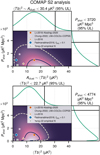 |
Fig. 2 Likelihood contours and marginalized probability distributions for the clustering and shot-noise amplitudes of the CO power spectrum, conditioned on COMAP Season 2 data, in b- and veff-agnostic (upper) and -informed (lower) analyses. Black solid lines plotted with the 1D marginalized distributions indicate the 95% upper limits for each parameter. The solid and dashed 2D contours are meant to encompass 39% and 86% of the probability mass (delineated at Δχ2 = {1, 4} relative to the minimum χ2, corresponding to 1σ and 2σ for 2D Gaussians). We show the clustering and shot noise amplitudes for a subset of the models plotted in Fig. 1. Models shown in Fig. 1 but not shown here have values of Aclust or ⟨T b⟩2 well beyond the 2σ regions shown. |
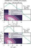 |
Fig. 3 Same as Fig. 2, but with a combination of COMAP Season 2 and COPSS data conditioning the likelihood. |
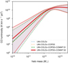 |
Fig. 4 68% intervals (lighter curves) and median values (darker curves) for |
![Mathematical equation: $\[L_{\mathrm{CO}}^{\prime}(M_{h})\]$](/articles/aa/full_html/2024/11/aa51122-24/aa51122-24-eq19.png)
3.2 Five-parameter analysis
Figs. 4 and 5 summarize the results of our five-parameter analysis in terms of derived quantities; we also show the posterior distributions in the original parameter space in Sect. D. First, comparing the “UM+COLDz” distribution with “UM+COLDz+COPSS+COMAP S1”, we do not see tangible differences in the derived quantities. The COPSS data on their own push the parameter space towards slightly higher σ, lower A (so a steeper faint-end slope for the L(Mh) relation), and overall a brighter signal as shown in the posteriors for ⟨T b⟩ and Pshot. However, the COMAP Season 1 non-detection essentially reverses many of these changes, even suggesting a slightly dimmer faint end of the halo mass–CO luminosity relation. None of these changes have great implications in terms of astrophysical understanding, given the low sensitivity of these datasets and the likely dominant influence of noise fluctuations on these results.
The COMAP Season 2 results push expectations for the signal back up, albeit only marginally. By pushing the double power law pivot mass M to lower values and pushing A (the opposite of the faint-end slope) to higher values, the COMAP Season 2 analysis suggests a brighter population of low-mass halos than our previous data would allow, as shown in Fig. 4. This is also apparent in Fig. 5, where the “UM+COLDz+COPSS+COMAP S2” posteriors for the derived quantities ⟨T b⟩, and Pshot show a systematic shift towards higher ⟨T b⟩ – for the first time markedly pushing away from the lower limit implied by the UM+COLDz distribution – in addition to a less extended right tail for Pshot.
As with the other datasets, the changes described above have little physical significance, since after all even the COMAP Season 2 results contain nothing that we would characterize as a firm detection. However, the nominal significance of the sensitivity achieved is worth noting. These shifts in the posterior distribution suggest that the COMAP Pathfinder survey is approaching the point of making statements about the faint end of the CO luminosity function by accessing its contribution to the clustering of CO emissivity on cosmological scales, something no other survey on the horizon will do.
Finally, we note that the “UM+COLDz+COPSS+COMAP S2” estimate for ⟨T⟩ – which incorporates prior information and should not be considered a COMAP “detection” of any kind – is ![Mathematical equation: $\[0.72_{-0.30}^{+0.45}\]$](/articles/aa/full_html/2024/11/aa51122-24/aa51122-24-eq20.png) μK. This corresponds to a cosmic molecular gas density of
μK. This corresponds to a cosmic molecular gas density of ![Mathematical equation: $\[\rho_{\mathrm{H} 2}=5.0_{-2.1}^{+3.1} \times 10^{7} M_{\odot} ~\mathrm{Mpc}^{-3}\]$](/articles/aa/full_html/2024/11/aa51122-24/aa51122-24-eq21.png) , which we discuss further in the next section.
, which we discuss further in the next section.
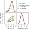 |
Fig. 5 Derived posterior distributions for ⟨T b⟩ and Pshot based on the five-parameter MCMC described in the main text. The inner (outer) contours of each distribution show the 1σ (2σ) confidence regions. |
4 Discussion
Phrased in terms of constraints on ρH2, the COMAP Season 2 results show the progress that COMAP – and thus single-dish CO LIM as a technique – has made in growing into an independent probe of cosmological CO emission and thus of cosmic molecular gas content. We illustrate this graphically in Fig. 6, showing the present work’s COMAP results in the context of previous work. The results from prior literature are mostly the same as those Chung et al. (2022) collated for their Fig. 9.
Deep surveys have leveraged community interferometers to observe pencil beam volumes and identify CO line emission candidates from the integrated data cubes in a serendipitous fashion. Of surveys used for such untargeted line searches, only the COLDz survey previously discussed in Sect. 2.3 directly observes high-redshift CO(1–0) line emission.
Two other deep interferometric surveys – the ALMA SPECtroscopic Survey in the Hubble Ultra Deep Field (ASPECS; Decarli et al. 2020) and the Plateau de Bure Highz Blue Sequence Survey 2 (PHIBBS2; Lenkić et al. 2020) – include 3 mm observations sensitive to a range of CO lines including CO(3–2) at z ≈ 2–33. These constraints on CO luminosity density, and thus ρH2, are subject to an additional conversion to CO(1–0) luminosity from higher-J CO lines.
Community interferometers have also hosted key pilot small-scale CO LIM surveys, namely the previously mentioned COPSS and mmIME.
As an additional reference point, we also overplot the best-fitting model from Garratt et al. (2021) to stacked 850 μm luminosities of near-infrared selected galaxies at redshifts 0–2.5. That work took advantage of a tight empirical correlation identified by Scoville et al. (2016) between the 850 μm luminosity and CO(1–0) luminosity of both low-redshift galaxies and z ~ 2 submillimeter galaxies. This stands in contrast to the other results assembled, which directly survey CO lines in some fashion, although not always specifically CO(1–0).
While COMAP Season 2 data are in weak disagreement with the COPSS results, this does not translate into a disagreement in the space of ρH2. This is due to the way in which Keating et al. (2016) derived ρH2 from the COPSS results. The derivation involved a number of stringent model assumptions including a linear relation between halo mass and CO luminosity, a linear relation between halo mass and molecular gas mass fraction, and the introduction of a prior on the log-normal scatter σ that suppressed the preferred amount of CO luminosity per halo mass versus what an unconstrained analysis would have found. Such assumptions motivate the analyses carried out in the present work, analysing multiple datasets through common modeling frameworks with shared assumptions. Compare, for instance, our own COPSS re-analysis which found an upper limit of ρH2 < 6.4–7.4 × 10⁸ M⊙ Mpc−3 in Sect. 3.1, versus our own COMAP S2 upper limit of ρH2 < 1.6 × 10⁸ M⊙ Mpc−3.
As mentioned at the end of Sect. 3.2, our best estimate for ρH2 when combining COMAP Season 2 with external prior information is ![Mathematical equation: $\[\rho_{\mathrm{H} 2}=5.0_{-2.1}^{+3.1} \times 10^{7} M_{\odot} ~\mathrm{Mpc}^{-3}\]$](/articles/aa/full_html/2024/11/aa51122-24/aa51122-24-eq22.png) . We show in Fig. 6 that this “UM+COLDz+COPSS+COMAP S2” estimate lies squarely between constraints from CO line searches, which cluster lower, and constraints from interferometric CO LIM surveys, which cluster higher. These two different families of experiments informed two different sets of forecasts of COMAP Pathfinder five-year results in Chung et al. (2022), one using the fiducial data-driven “UM+COLDz+COPSS” model4 and the other using the Li et al. (2016)–Keating et al. (2020) model originally formulated to explain mmIME results. Our best estimate thus also lies between these two models from COMAP Early Science and the forecasts that used them, which we show alongside previous and current results in Fig. 7.
. We show in Fig. 6 that this “UM+COLDz+COPSS+COMAP S2” estimate lies squarely between constraints from CO line searches, which cluster lower, and constraints from interferometric CO LIM surveys, which cluster higher. These two different families of experiments informed two different sets of forecasts of COMAP Pathfinder five-year results in Chung et al. (2022), one using the fiducial data-driven “UM+COLDz+COPSS” model4 and the other using the Li et al. (2016)–Keating et al. (2020) model originally formulated to explain mmIME results. Our best estimate thus also lies between these two models from COMAP Early Science and the forecasts that used them, which we show alongside previous and current results in Fig. 7.
As COMAP continues to move forward as a single-dish experiment, its large-scale imaging will complement interferometric surveys in important ways. This includes not only COPSS and mmIME but also resolved line candidate searches including ASPECS, since COMAP relies on statistical large-scale fluctuations rather than individual sources. For example, ASPECS-Pilot detected 14 high-redshift [C II] line candidates (Aravena et al. 2016) only to show in the subsequent ASPECS Large Program observations that every single one was spurious (Uzgil et al. 2021). The importance of having independent single-dish LIM experiments similar to COMAP in the conversation will only increase as COMAP accrues further data.
The other important focus of COMAP that is salient to the wider landscape of CO abundance measurements is its focus on low-J CO lines, specifically CO(1–0) at z ~ 3 in the case of the Pathfinder survey. For example, comparing the results of Garratt et al. (2021) against those of ASPECS or PHIBBS2 would require accounting for not only uncertainties in quantities such as αCO, but also the respective conversion from the original measurement into CO(1–0) luminosity density – the Scoville et al. (2016) 850 μm–CO(1–0) conversion in the case of Garratt et al. (2021), and the conversion to CO(1–0) from higher-J CO lines observed by ASPECS and PHIBBS2 (though for ASPECS see Riechers et al. 2020). Future COMAP constraints will entirely bypass this last uncertainty by directly constraining the CO(1–0) luminosity density – and across all faint and bright galaxies in the survey volume, not constrained to any specific galaxy selection.
For now our best estimates remain consistent with all experiments, but our sensitivity to the clustering of CO has clearly improved to the point of providing upward revisions to expectations for the average CO luminosities of low-mass halos. While the current sensitivities of COMAP data to the tracer bias and average line temperature are at best marginal against our informative priors, they will continue to grow as we accrue more data. As Lunde et al. (2024) note and as we have already noted in the Introduction, the COMAP Pathfinder achieved nearly an order-of-magnitude increase in power spectrum sensitivity per k-bin despite only a 3.4× increase in raw data volume. With continued improvements in data cleaning and analysis, we remain optimistic that the amount of usable data will increase nonlinearly with further observing seasons and allow the COMAP Pathfinder to meet its targets for five-year sensitivities. As it does so, the resulting constraints will readily lend itself to very straightforward joint analyses with other measurements of cosmic CO(1–0) emissivity or molecular gas content in the vein of other LIM surveys, line scan surveys, or even analyses similar to that of Garratt et al. (2021), enhancing our understanding of how the rise and fall of cosmic star-forming gas relates to its depletion through the rise and fall of cosmic star formation activity.
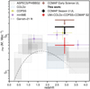 |
Fig. 6 Constraints on the cosmic molecular gas mass density ρH2 based on CO abundance measurements across redshifts 0–4. We show COMAP Season 1 and Season 2 constraints on ⟨T⟩ converted based on Eq. (13), including both the two-parameter analysis upper limit and the five-parameter UM+COLDz+COPSS+COMAP S2 result. For comparison, we also show past results from untargeted interferometric CO line searches (boxes) – ASPECS (Decarli et al. 2020), PHIBBS2 (Lenkić et al. 2020), and COLDz (Riechers et al. 2019) – as well as interferometric CO LIM surveys (uncapped error bars) – COPSS (Keating et al. 2016) and mmIME (Keating et al. 2020). In addition, we show a best-fit model describing results from stacked 850 μm luminosities of galaxies at redshifts 0–2.5 (Garratt et al. 2021). All results use αCO = 3.6 M⊙ (K km s−1 pc−2)−1 (cf. Daddi et al. 2010) except COPSS, which uses a conversion of αCO = 4.3 M⊙ (K km s−1 pc−2)−1 (cf. Bolatto et al. 2013), and Garratt et al. (2021), who use αCO = 6.5 M⊙ (K km s−1 pc−2)−1 as promoted by Scoville et al. (2016). |
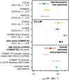 |
Fig. 7 Constraints on ρH2 just before “cosmic noon”, showing 95% upper limits and confidence intervals standardized to 68% when possible. In addition to constraints shown before in Fig. 6 from line searches (Riechers et al. 2019; Lenkić et al. 2020; Decarli et al. 2020), previous CO LIM analyses (Keating et al. 2016, 2020; Chung et al. 2022), and the present work, we also show COMAP Pathfinder 5-year forecasts from Chung et al. (2022). |
5 Conclusions
With the above results and discussion, we now have firm answers to the questions posed in the Introduction to this work:
“How much does the increased data volume improve constraints on the clustering and shot noise power of cosmological CO(1–0) emission at z ~ 3?” The COMAP Season 2 dataset represents a five-fold improvement in upper bounds on CO shot noise power and a halving of the upper bound on the CO clustering amplitude over COMAP Early Science. Specifically, our COMAP standalone upper limits for Pshot have evolved from 1.9–2.4 × 10³ μK2 Mpc3 to 3.7–4.9 × 10³ μK2 Mpc3 (depending on assumptions around astrophysical line broadening). This increased sensitivity introduces tension against the previous COPSS result, which will evolve with future analyses. Meanwhile, our Season 2 upper limit of ⟨T⟩ < 2.4 μK translates to ρH 2 < 1.6 × 10⁸ M⊙ Mpc−3 given further assumptions about the relation between CO luminosity and molecular gas mass.
“Can COMAP Season 2 results better constrain the empirical connection between CO emission and the underlying structures of dark matter?” While COMAP Season 2 data only provide marginal improvements in constraining this connection, we see hints of the COMAP Pathfinder’s basic capability in capturing the clustering of low-mass CO emitters in ways that other experiments cannot.
The present work has taken an extremely conservative approach to high-level analysis, with generic models for either the power spectrum or the halo–CO connection. By making even stronger model assumptions we can make statements about semi-analytic models of galaxy formation and the connection between star formation activity and molecular gas content (cf. Breysse et al. 2022). We leave this to a future collaboration work currently in preparation.
The outlook for the COMAP Pathfinder remains strongly positive as it continues past 3 years of data acquisition. The improvements demonstrated in Season 2, not only in observing efficiency but also in data cleaning and processing as demonstrated by the papers that this work accompanies (Lunde et al. 2024; Stutzer et al. 2024), will continue to grow with further Pathfinder operations. The collaboration thus continues to be on track for the outcome forecast by Chung et al. (2022): a highsignificance detection of cosmological CO clustering sometime in the next few years.
Acknowledgements
DTC was supported by a CITA/Dunlap Institute postdoctoral fellowship for much of this work. The Dunlap Institute is funded through an endowment established by the David Dunlap family and the University of Toronto. The University of Toronto operates on the traditional land of the Huron-Wendat, the Seneca, and most recently, the Mississaugas of the Credit River; DTC is grateful to have the opportunity to work on this land. Research in Canada is supported by NSERC and CIFAR. This material is based upon work supported by the National Science Foundation under Grant Nos. 1517108, 1517288, 1517598, 1518282, 1910999, and 2206834, as well as by the Keck Institute for Space Studies under “The First Billion Years: A Technical Development Program for Spectral Line Observations”. Parts of the work were carried out at the Jet Propulsion Laboratory, California Institute of Technology, under a contract with the National Aeronautics and Space Administration. PCB acknowledges support from the James Arthur Postdoctoral Fellowship during the writing of this work. We acknowledge and thank the support from the Research Council of Norway through grants 251328 and 274990, and from the European Research Council (ERC) under the Horizon 2020 Research and Innovation Program (grant agreements 772253 bits2cosmology and 819478 Cosmoglobe). HP acknowledges support from the Swiss National Science Foundation via Ambizione Grant PZ00P2_179934. This work was supported in part by the National Research Foundation of Korea (NRF) grant funded by the Korean government (MSIT, No. RS-2024-00340759). This study uses the Scientific color map acton (Crameri 2021) to prevent visual distortion of the data and exclusion of readers with color-vision deficiencies (Crameri et al. 2020). As in Chung et al. (2022) we thank Riccardo Pavesi for access to the COLDz ABC posterior sample used in this work. Many thanks also to George Stein for running and making available the original peak-patch simulations for use with the COMAP Pathfinder survey. This research made use of NASA’s Astrophysics Data System Bibliographic Services. Some of the methods for this work were originally tested on the Sherlock cluster; DTC would like to thank Stanford University and the Stanford Research Computing Center for providing computational resources and support that contributed to these research results. This work was first presented at the Line Intensity Mapping 2024 conference held in Urbana, Illinois; we thank Joaquin Vieira and the other organizers for their hospitality and the participants for useful discussions. Finally, we thank the anonymous referee for their constructive input towards the final state of this article.
Appendix A Alternative presentation of observed power spectra
Fig. A.1 provides an alternate presentation of the LIM observations shown in Fig. 1 as part of Sect. 2.1. Namely, we represent all P(k) datasets not as upper limits given positivity priors, and instead as data points on a linear scale. In this case we take the feed or feed-group pseudo cross-power spectrum data ![Mathematical equation: $\[\tilde{C}(k)\]$](/articles/aa/full_html/2024/11/aa51122-24/aa51122-24-eq23.png) derived in Ihle et al. (2022) and Stutzer et al. (2024) as the best COMAP Season 1 and Season 2 estimates for the astrophysical P(k). We also show credible ranges of P(k) values from the two-parameter analyses of Sect. 3 rather than specific models as in Fig. 1.
derived in Ihle et al. (2022) and Stutzer et al. (2024) as the best COMAP Season 1 and Season 2 estimates for the astrophysical P(k). We also show credible ranges of P(k) values from the two-parameter analyses of Sect. 3 rather than specific models as in Fig. 1.
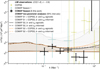 |
Fig. A.1 Same as Fig. 1, but with all LIM P(k) results shown with 1σ uncertainties per k-bin and on a linear scale. Furthermore, instead of the specific models shown in Fig. 1, we show the typical range of allowable power spectrum values based on the two-parameter analyses of Sect. 3, with the b-/veff-informed variations showing attenuation for line broadening left uncorrected. These allowable ranges shown should not be taken to represent a detection as they assume non-negative P(k) values by definition. |
While the Early Science work of Chung et al. (2022) represented COMAP Season 1 and COPSS data as co-added results across their respective k-ranges, we will not adopt such representation in future work. Inter-bin correlations, interacting with imposition of a positivity prior on the co-added result versus on the individual P(k) points, could result in differences between co-added and per-bin results impossible to make sense of. For COMAP Season 2 data, we have explicitly verified that interbin correlations are ≲ 10% for our chosen k-binning (Stutzer et al. 2024). Even so, the choice of how to represent a co-added result is fraught with many choices with respect to the averaging scheme, the central k-value, and can lead to misleading visual comparisons when plotting model power spectra alongside coadded results without the same weighting used to average the observed power spectra.
Appendix B Derivation of “UM” priors by Chung et al. (2022), recapped
In this section, we review the procedures followed by Chung et al. (2022) to derive the “UM” priors for {A, B, C, M} that serve as our starting point for the procedures of Sect. 2.3.
The UNIVERSEMACHINE framework used by Behroozi et al. (2019) takes the maximum circular velocity at peak halo mass ![Mathematical equation: $\[v_{M_{\text {peak }}}\]$](/articles/aa/full_html/2024/11/aa51122-24/aa51122-24-eq24.png) as the key quantity describing the depth of the dark matter halo potential to then relate to a minimal model connecting star formation activity with halo accretion and merger histories. The best-fit model describes the average SFR of star-forming galaxies as a function of
as the key quantity describing the depth of the dark matter halo potential to then relate to a minimal model connecting star formation activity with halo accretion and merger histories. The best-fit model describes the average SFR of star-forming galaxies as a function of ![Mathematical equation: $\[v_{M_{\text {peak }}}\]$](/articles/aa/full_html/2024/11/aa51122-24/aa51122-24-eq25.png) , taking the form of the sum of a double power law with a Gaussian function:
, taking the form of the sum of a double power law with a Gaussian function:
![Mathematical equation: $\[\frac{\left\langle\mathrm{SFR}_{\mathrm{SF}}\right\rangle\left(v_{M_{\text {peak }}}\right)}{M_{\odot} ~\mathrm{yr}^{-1}}=\epsilon\left[\frac{1}{v^{\alpha_\mathrm{UM}}+v^{\beta_\mathrm{UM}}}+\gamma \exp \left(-\frac{\log ^{2} v}{2 \delta^{2}}\right)\right],\]$](/articles/aa/full_html/2024/11/aa51122-24/aa51122-24-eq26.png) (B.1)
(B.1)
where
![Mathematical equation: $\[v=\frac{v_{M_{\text {peak }}}}{V\left[\mathrm{~km} \mathrm{~s}^{-1}\right]}.\]$](/articles/aa/full_html/2024/11/aa51122-24/aa51122-24-eq27.png) (B.2)
(B.2)
Here αUM, βUM, γ, δ, ε, and V are all UNIVERSEMACHINE parameters to be determined in the model fitting. (We follow Chung et al. (2022) and add “UM” subscripts to α and β from Behroozi et al. 2019 to disambiguate these specifically as UNIVERSEMACHINE parameters.) For our purposes of deriving a simple parameterization of ![Mathematical equation: $\[L_{\mathrm{CO}}^{\prime}(M_{h})\]$](/articles/aa/full_html/2024/11/aa51122-24/aa51122-24-eq28.png) , we neglect the Gaussian function (i.e., γ ≈ 0), leaving only the double power law.
, we neglect the Gaussian function (i.e., γ ≈ 0), leaving only the double power law.
We wish to leverage this into a relation between halo mass and CO luminosity. First, we relate halo mass to ![Mathematical equation: $\[v_{M_{\text {peak }}}\]$](/articles/aa/full_html/2024/11/aa51122-24/aa51122-24-eq29.png) through an approximate relation given by Behroozi et al. (2019):
through an approximate relation given by Behroozi et al. (2019):
![Mathematical equation: $\[v_{M_{\text {peak }}}\left(M_{h}\right)=\left(200 \mathrm{~km} \mathrm{~s}^{-1}\right)\left[\frac{M_{h}}{M_{200 \mathrm{~km} / \mathrm{s}}(a)}\right]^{0.3},\]$](/articles/aa/full_html/2024/11/aa51122-24/aa51122-24-eq30.png) (B.3)
(B.3)
where a = 1/(1 + z) is the scale factor at redshift z, and
![Mathematical equation: $\[M_{200 \mathrm{~km} / \mathrm{s}}=\frac{1.64 \times 10^{12} M_{\odot}}{(a / 0.378)^{-0.142}+(a / 0.378)^{-1.79}}.\]$](/articles/aa/full_html/2024/11/aa51122-24/aa51122-24-eq31.png) (B.4)
(B.4)
Next, we relate SFR to CO luminosity in the same fashion as Li et al. (2016), which is through a series of scaling relations. First we take the bolometric infrared luminosity to be a proxy for SFR:
![Mathematical equation: $\[\frac{\mathrm{SFR}}{M_{\odot} ~\mathrm{yr}^{-1}}=\delta_{\mathrm{MF}} \times 10^{-10}\left(\frac{L_{\mathrm{IR}}}{L_{\odot}}\right),\]$](/articles/aa/full_html/2024/11/aa51122-24/aa51122-24-eq32.png) (B.5)
(B.5)
given some scaling factor δMF whose value depends on the initial mass function (IMF). We set this to 1 as in Li et al. (2016).
Observational literature then allows us to empirically relate IR luminosity and CO luminosity, with the common form being a single power law converting between the two (as in the review of Carilli & Walter 2013):
![Mathematical equation: $\[\log~ L_{\mathrm{IR}}=\alpha ~\log~ L_{\mathrm{CO}}^{\prime}+\beta,\]$](/articles/aa/full_html/2024/11/aa51122-24/aa51122-24-eq33.png) (B.6)
(B.6)
where for CO(1–0),
![Mathematical equation: $\[\frac{L_{\mathrm{CO}}}{L_{\odot}}=4.9 \times 10^{-5} \frac{L_{\mathrm{CO}}^{\prime}}{\mathrm{K} ~\mathrm{km} \mathrm{s}^{-1} ~\mathrm{pc}^{2}}.\]$](/articles/aa/full_html/2024/11/aa51122-24/aa51122-24-eq34.png) (B.7)
(B.7)
These scaling relations introduce the additional parameters of α, β, and δMF beyond the parameters αUM, βUM, ε, and V describing the double power law portion of Equation B.1.
Under the approximation of α ≈ 1 (or at least α ≪ 1 and α ≫ 1), the composition of all of the above scaling relations is approximately described by the double power law form given in Equation 6, and the parameters of the above relations transform into the parameters of Equation 6 as follows:
![Mathematical equation: $\[A=0.3 \alpha_{\mathrm{UM}} / \alpha;\]$](/articles/aa/full_html/2024/11/aa51122-24/aa51122-24-eq35.png) (B.8)
(B.8)
![Mathematical equation: $\[B=0.3 \beta_{\mathrm{UM}} / \alpha;\]$](/articles/aa/full_html/2024/11/aa51122-24/aa51122-24-eq36.png) (B.9)
(B.9)
![Mathematical equation: $\[\log~ C=\left(10-\log ~\delta_{\mathrm{MF}}-\beta+\log \epsilon\right) / \alpha;\]$](/articles/aa/full_html/2024/11/aa51122-24/aa51122-24-eq37.png) (B.10)
(B.10)
![Mathematical equation: $\[\log ~\left(M / M_{\odot}\right)=~\log~ M_{200 \mathrm{~km} / \mathrm{s}}+(10 / 3) ~\log~ (V / 200).\]$](/articles/aa/full_html/2024/11/aa51122-24/aa51122-24-eq38.png) (B.11)
(B.11)
These transformations allow us to derive priors for {A, B, C, M} by propagating the priors on α, β, and δMF from Li et al. (2016) – namely α = 1.17 ± 0.37, β = 0.21 ± 3.74, and log δMF = 0.0 ± 0.5 – and the 68% interval around the best-fit values of the other parameters from Behroozi et al. (2019). (We used the best-fit model from the Early Data Release, fixed at z = 2.4 to match the median redshift of the COLDz survey. We do not consider the changes between this and the official Data Release 1 large enough to recalculate our priors. Along similar lines, any redshift evolution in this model is not the dominant source of model uncertainty.) The resulting initial priors on {A, B, C, M} are as described in the main text.
The additional prior of σ = 0.4 ± 0.2 (dex) derives its central value from the total scatter of 0.37 dex present in the CO model of Li et al. (2016); this level of log-normal scatter is typical for correlations involving galaxy properties such as SFR, as Li et al. (2016) note.
Appendix C The conversion between molecular gas density and CO luminosity density
The mass-to-light ratio αCO in Equation 13 relates the CO luminosity ![Mathematical equation: $\[L_{\mathrm{CO}}^{\prime}\]$](/articles/aa/full_html/2024/11/aa51122-24/aa51122-24-eq39.png) of a galaxy, in units of velocity- and area-integrated brightness temperature, to the molecular gas mass Mmol in that galaxy. This ratio depends intensely on many environmental, morphological, and other variables unique to each galaxy, but it is common to assume a single value across an entire survey.
of a galaxy, in units of velocity- and area-integrated brightness temperature, to the molecular gas mass Mmol in that galaxy. This ratio depends intensely on many environmental, morphological, and other variables unique to each galaxy, but it is common to assume a single value across an entire survey.
One can equivalently assume a conversion between the H2 column density (NH2) and the velocity-integrated (but not areaintegrated) CO brightness temperature WCO. The conventional notation for that ratio is XCO:
![Mathematical equation: $\[N_{\mathrm{H} 2}=X_{\mathrm{CO}} W_{\mathrm{CO}}.\]$](/articles/aa/full_html/2024/11/aa51122-24/aa51122-24-eq40.png) (C.1)
(C.1)
The scaling from NH2 to Mmol is the apparent size of the galaxy, with an additional correction of 1.36 (per Bolatto et al. 2013) for the presence of heavy elements in molecular gas beyond diatomic hydrogen. But the scaling from WCO to ![Mathematical equation: $\[L_{\mathrm{CO}}^{\prime}\]$](/articles/aa/full_html/2024/11/aa51122-24/aa51122-24-eq41.png) is also the apparent size of the galaxy, meaning that αCO and XCO are completely equivalent except for the molecular mass of diatomic hydrogen mH2 and the aforementioned factor of 1.36:
is also the apparent size of the galaxy, meaning that αCO and XCO are completely equivalent except for the molecular mass of diatomic hydrogen mH2 and the aforementioned factor of 1.36:
![Mathematical equation: $\[\alpha_{\mathrm{CO}}=\frac{M_{\mathrm{mol}}}{L_{\mathrm{CO}}^{\prime}}=\frac{1.36 m_{\mathrm{H} 2} N_{\mathrm{H} 2}}{W_{\mathrm{CO}}}=1.36 m_{\mathrm{H} 2} X_{\mathrm{CO}}.\]$](/articles/aa/full_html/2024/11/aa51122-24/aa51122-24-eq42.png) (C.2)
(C.2)
From here it is straightforward to find the numerical conversion in terms of the conventional units of each ratio:
![Mathematical equation: $\[\frac{\alpha_{\mathrm{CO}}}{M_{\odot} /\left(\mathrm{K} ~\mathrm{km} ~\mathrm{s}^{-1} ~\mathrm{pc}^{2}\right)}=2.18 \times 10^{-20} \times \frac{X_{\mathrm{CO}}}{\mathrm{cm}^{-2} /\left(\mathrm{K} ~\mathrm{km} ~\mathrm{s}^{-1}\right)}.\]$](/articles/aa/full_html/2024/11/aa51122-24/aa51122-24-eq43.png) (C.3)
(C.3)
(Note that the review of Carilli & Walter (2013) gives XCO/αCO = 4.6 × 10¹⁰ pc2 cm−2 M⊙−1; this appears to be a typo, as the numerical value before units should be 4.6 × 10¹⁹.)
Although one can attempt to understand αCO or XCO from various analytical and numerical starting points in theoretical astrophysics, empirical considerations largely drive the choice of specific values of this conversion in interpretations of extragalactic CO surveys.
The review of Bolatto et al. (2013) recommends a value of XCO = 2 × 1020 cm−2/(K km s−1), or equivalently αCO = 4.3 M⊙/(K km s−1 pc2), for normal solar-metallicity disk galaxies, based on the values observed in our own Galactic disk (which range between 0.7 and 4.2 in XCO/[1020 cm−2/(K km s−1)] in the references compiled in Table 1 of Bolatto et al. 2013). For massive starbursts and ultra-luminous infrared galaxies the value would scale down with increasing total gas surface density, with Bolatto et al. (2013) claiming a value one-fifth that of the Galactic value as a typical model result.
Many high-redshift CO surveys, including the interferometric line searches showcased in Fig. 6 and LIM surveys including the COMAP Pathfinder, adopt a value of αCO = 3.6 M⊙ (K km s−1 pc−2)−1 based on the work of Daddi et al. (2010), which undertook resolved interferometric imaging of three z ~ 1.5 normal star-forming galaxies. This is slightly lower than (but still within observational uncertainty of) the Galactic value but much higher than the expectation outlined above for starbursts.
Scoville et al. (2016) assume a higher value of αCO = 6.5 M⊙/(K km s−1 pc2) specifically in the context of global observations of galaxies, both normal star-forming galaxies and massive starbursts. Scoville et al. (2016) argue against giving too much weight to the γ-ray emission analysis results out of the XCO values compiled by Bolatto et al. (2013) (which do skew on the lower side of the final recommendation of that work), further arguing that XCO values obtained in resolved studies of starbursts may not be appropriate for global characterization.
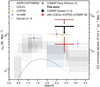 |
Fig. C.1 Same as Fig. 6, but with the COPSS (Keating et al. 2016) and Garratt et al. (2021) results re-normalized to match the αCO value of αCO = 3.6 M⊙ (K km s−1 pc−2)−1 assumed by all other works shown. We also show what CO luminosity density the values of ρH2 correspond to without the factor of αCO. |
Other works make other assumptions about appropriate values of this conversion. Scoville et al. (2016) note that the analysis of Draine et al. (2007) supports an even higher value of XCO = 4 × 1020 cm−2/(K km s−1) for a sample of nearby galaxies with near- and far-infrared observations. Meanwhile, the empirical relation of Accurso et al. (2017) incorporates dependences on metallicity and main sequence offset, and assigns αCO values to some observed galaxies as high as four times that of the Galactic value.
Ultimately, the chosen value of αCO is just one of a large number of assumptions made by a survey about the target galaxy population, among other assumptions including (for example, in interferometric line searches) the faint-end slope and cutoff of the luminosity function. Given this, we make no attempt to alter results to normalise around a single value of αCO in the main text as the different values chosen by different surveys reflect their best understanding of how the CO content surveyed by the respective surveys corresponds to molecular gas content.
However, if we wish to compare the actual CO luminosity densities claimed by each survey on equal footing, then the different values of αCO serve as a distraction. As such, we present in Fig. C.1 an alternate version of Fig. 6, wherein we have renormalized the results of Keating et al. (2016) and Garratt et al. (2021) to match the Daddi et al. (2010) value of αCO used by all other works. We neglect any other assumptions about the surveyed galaxy population in the process so even this comparison is not necessarily entirely even.
Appendix D Full five-parameter MCMC posterior distributions
In Fig. D.1 we show the full five-parameter posterior distributions from the analysis of Sect. 2.3, from which we obtain distributions for the derived quantities shown in Sect. 3.2. Compared to Fig. 5, the changes due to COMAP Season 2 data are more subtle in this higher-dimensional space but nonetheless discernible.
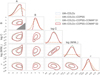 |
Fig. D.1 MCMC posterior distributions for the five parameters of our |
![Mathematical equation: $\[L_{\mathrm{CO}}^{\prime}\left(M_{h}\right)\]$](/articles/aa/full_html/2024/11/aa51122-24/aa51122-24-eq44.png)
References
- Accurso, G., Saintonge, A., Catinella, B., et al. 2017, MNRAS, 470, 4750 [NASA ADS] [Google Scholar]
- Aravena, M., Decarli, R., Walter, F., et al. 2016, ApJ, 833, 71 [NASA ADS] [CrossRef] [Google Scholar]
- Behroozi, P. S., Wechsler, R. H., & Conroy, C. 2013a, ApJ, 762, L31 [NASA ADS] [CrossRef] [Google Scholar]
- Behroozi, P. S., Wechsler, R. H., & Conroy, C. 2013b, ApJ, 770, 57 [NASA ADS] [CrossRef] [Google Scholar]
- Behroozi, P., Wechsler, R. H., Hearin, A. P., & Conroy, C. 2019, MNRAS, 488, 3143 [NASA ADS] [CrossRef] [Google Scholar]
- Bernal, J. L., & Kovetz, E. D. 2022, A&A Rev., 30, 5 [NASA ADS] [CrossRef] [Google Scholar]
- Bolatto, A. D., Wolfire, M., & Leroy, A. K. 2013, ARA&A, 51, 207 [CrossRef] [Google Scholar]
- Boogaard, L. A., Decarli, R., Walter, F., et al. 2023, ApJ, 945, 111 [NASA ADS] [CrossRef] [Google Scholar]
- Breysse, P. C., Yang, S., Somerville, R. S., et al. 2022, ApJ, 929, 30 [NASA ADS] [CrossRef] [Google Scholar]
- Carilli, C. L., & Walter, F. 2013, ARA&A, 51, 105 [NASA ADS] [CrossRef] [Google Scholar]
- Chung, D. T., Breysse, P. C., Ihle, H. T., et al. 2021, ApJ, 923, 188 [NASA ADS] [CrossRef] [Google Scholar]
- Chung, D. T., Breysse, P. C., Cleary, K. A., et al. 2022, ApJ, 933, 186 [NASA ADS] [CrossRef] [Google Scholar]
- Cleary, K. A., Borowska, J., Breysse, P. C., et al. 2022, ApJ, 933, 182 [NASA ADS] [CrossRef] [Google Scholar]
- Crameri, F. 2021, https://doi.org/10.5281/zenodo.1243862 [Google Scholar]
- Crameri, F., Shephard, G. E., & Heron, P. J. 2020, Nat. Commun., 11, 5444 [NASA ADS] [CrossRef] [Google Scholar]
- Daddi, E., Bournaud, F., Walter, F., et al. 2010, ApJ, 713, 686 [NASA ADS] [CrossRef] [Google Scholar]
- Decarli, R., Aravena, M., Boogaard, L., et al. 2020, ApJ, 902, 110 [Google Scholar]
- Draine, B. T., Dale, D. A., Bendo, G., et al. 2007, ApJ, 663, 866 [NASA ADS] [CrossRef] [Google Scholar]
- Förster Schreiber, N. M., & Wuyts, S. 2020, ARA&A, 58, 661 [Google Scholar]
- Foss, M. K., Ihle, H. T., Borowska, J., et al. 2022, ApJ, 933, 184 [NASA ADS] [CrossRef] [Google Scholar]
- Garratt, T. K., Coppin, K. E. K., Geach, J. E., et al. 2021, ApJ, 912, 62 [NASA ADS] [CrossRef] [Google Scholar]
- Hamilton, A. J. S. 1998, in The Evolving Universe, ed. D. Hamilton, Astrophysics and Space Science Library, 231, 185 [NASA ADS] [CrossRef] [Google Scholar]
- Ihle, H. T., Borowska, J., Cleary, K. A., et al. 2022, ApJ, 933, 185 [NASA ADS] [CrossRef] [Google Scholar]
- Kaiser, N. 1987, MNRAS, 227, 1 [Google Scholar]
- Kamenetzky, J., Rangwala, N., Glenn, J., Maloney, P. R., & Conley, A. 2016, ApJ, 829, 93 [Google Scholar]
- Keating, G. K., Marrone, D. P., Bower, G. C., et al. 2016, ApJ, 830, 34 [NASA ADS] [CrossRef] [Google Scholar]
- Keating, G. K., Marrone, D. P., Bower, G. C., & Keenan, R. P. 2020, ApJ, 901, 141 [NASA ADS] [CrossRef] [Google Scholar]
- Kovetz, E., Breysse, P. C., Lidz, A., et al. 2019, BAAS, 51, 101 [NASA ADS] [Google Scholar]
- Lamb, J. W., Cleary, K. A., Woody, D. P., et al. 2022, ApJ, 933, 183 [NASA ADS] [CrossRef] [Google Scholar]
- Lenkić, L., Bolatto, A. D., Förster Schreiber, N. M., et al. 2020, AJ, 159, 190 [CrossRef] [Google Scholar]
- Li, T. Y., Wechsler, R. H., Devaraj, K., & Church, S. E. 2016, ApJ, 817, 169 [NASA ADS] [CrossRef] [Google Scholar]
- Lunde, J. G. S., Stutzer, N. O., Breysse, P. C., et al. 2024, A&A, 691, A335 (Paper I) [NASA ADS] [CrossRef] [EDP Sciences] [Google Scholar]
- Padmanabhan, H. 2018, MNRAS, 475, 1477 [NASA ADS] [CrossRef] [Google Scholar]
- Pavesi, R., Sharon, C. E., Riechers, D. A., et al. 2018, ApJ, 864, 49 [Google Scholar]
- Pullen, A. R., Chang, T.-C., Doré, O., & Lidz, A. 2013, ApJ, 768, 15 [NASA ADS] [CrossRef] [Google Scholar]
- Riechers, D. A., Boogaard, L. A., Decarli, R., et al. 2020, ApJ, 896, L21 [NASA ADS] [CrossRef] [Google Scholar]
- Riechers, D. A., Pavesi, R., Sharon, C. E., et al. 2019, ApJ, 872, 7 [Google Scholar]
- Scoville, N., Sheth, K., Aussel, H., et al. 2016, ApJ, 820, 83 [Google Scholar]
- Somerville, R. S., & Davé, R. 2015, ARA&A, 53, 51 [Google Scholar]
- Stein, G., Alvarez, M. A., & Bond, J. R. 2019, MNRAS, 483, 2236 [NASA ADS] [CrossRef] [Google Scholar]
- Stutzer, N. O., Lunde, J. G. S., Breysse, P. C., et al. 2024, A&A, 691, A336 (Paper II) [NASA ADS] [CrossRef] [EDP Sciences] [Google Scholar]
- Tinker, J., Kravtsov, A. V., Klypin, A., et al. 2008, ApJ, 688, 709 [Google Scholar]
- Uzgil, B. D., Oesch, P. A., Walter, F., et al. 2021, ApJ, 912, 67 [Google Scholar]
- Yang, S., Popping, G., Somerville, R. S., et al. 2022, ApJ, 929, 140 [NASA ADS] [CrossRef] [Google Scholar]
This approximates the likelihood as Gaussian and independent between k-bins, which we consider to be a reasonable approximation at least for COMAP Season 2 data. In obtaining the P(k) result, Stutzer et al. (2024) found that on average, any single k-bin correlated with any other k-bin at a level of ≲ 10%.
Curiously, however, the upward correction is similar between the COMAP S2 standalone analyses – in fact, it ends up slightly larger at 32%. This is not entirely insensible. Even small amounts of attenuation allowable within uncertainties at lower wavenumbers correspond to a large possible range of corrections for attenuation of the shot noise component, and this lever arm from low k to high k is larger with COMAP data alone than with COPSS data added to the analysis.
See also Riechers et al. (2020) and Boogaard et al. (2023), which iterate on the ASPECS results with complementary observations. Figure 10 of Boogaard et al. (2023) demonstrates that at z ≈ 2–3, these studies are both consistent with those discussed here, certainly within the expected behavior of noise (including cosmic variance).
Although this model originated from a data-driven prior that also used COPSS, the COLDz data clearly dominated the information content reflected in the prior. We see this again in the present work from the minimal difference between the “UM+COLDz” and “UM+COLDz+COPSS” posteriors in Sect. 3.2.
All Tables
All Figures
|
Fig. 1 COMAP Season 2 95% upper limits (given P(k) > 0) on the z ~ 3 CO(1–0) power spectrum, with analogous limits from COPSS (Keating et al. 2016) and COMAP Season 1 (Chung et al. 2022). Some k-bins in COPSS and COMAP Season 2 data show marginal excesses, influencing analyses in this work; we thus show 1σ intervals for these bins unlike in Stutzer et al. (2024). We also show predictions based on Chung et al. (2022), Padmanabhan (2018), Pullen et al. (2013), Li et al. (2016), and Yang et al. (2022), plus a variation on the Li et al. (2016) model from Keating et al. (2020), and the Keating et al. (2020) re-analysis of COPSS constraining clustering (triangles) and shot-noise amplitudes (dashed line). |
| In the text | |
|
Fig. 2 Likelihood contours and marginalized probability distributions for the clustering and shot-noise amplitudes of the CO power spectrum, conditioned on COMAP Season 2 data, in b- and veff-agnostic (upper) and -informed (lower) analyses. Black solid lines plotted with the 1D marginalized distributions indicate the 95% upper limits for each parameter. The solid and dashed 2D contours are meant to encompass 39% and 86% of the probability mass (delineated at Δχ2 = {1, 4} relative to the minimum χ2, corresponding to 1σ and 2σ for 2D Gaussians). We show the clustering and shot noise amplitudes for a subset of the models plotted in Fig. 1. Models shown in Fig. 1 but not shown here have values of Aclust or ⟨T b⟩2 well beyond the 2σ regions shown. |
| In the text | |
|
Fig. 3 Same as Fig. 2, but with a combination of COMAP Season 2 and COPSS data conditioning the likelihood. |
| In the text | |
|
Fig. 4 68% intervals (lighter curves) and median values (darker curves) for |
| In the text | |
|
Fig. 5 Derived posterior distributions for ⟨T b⟩ and Pshot based on the five-parameter MCMC described in the main text. The inner (outer) contours of each distribution show the 1σ (2σ) confidence regions. |
| In the text | |
|
Fig. 6 Constraints on the cosmic molecular gas mass density ρH2 based on CO abundance measurements across redshifts 0–4. We show COMAP Season 1 and Season 2 constraints on ⟨T⟩ converted based on Eq. (13), including both the two-parameter analysis upper limit and the five-parameter UM+COLDz+COPSS+COMAP S2 result. For comparison, we also show past results from untargeted interferometric CO line searches (boxes) – ASPECS (Decarli et al. 2020), PHIBBS2 (Lenkić et al. 2020), and COLDz (Riechers et al. 2019) – as well as interferometric CO LIM surveys (uncapped error bars) – COPSS (Keating et al. 2016) and mmIME (Keating et al. 2020). In addition, we show a best-fit model describing results from stacked 850 μm luminosities of galaxies at redshifts 0–2.5 (Garratt et al. 2021). All results use αCO = 3.6 M⊙ (K km s−1 pc−2)−1 (cf. Daddi et al. 2010) except COPSS, which uses a conversion of αCO = 4.3 M⊙ (K km s−1 pc−2)−1 (cf. Bolatto et al. 2013), and Garratt et al. (2021), who use αCO = 6.5 M⊙ (K km s−1 pc−2)−1 as promoted by Scoville et al. (2016). |
| In the text | |
|
Fig. 7 Constraints on ρH2 just before “cosmic noon”, showing 95% upper limits and confidence intervals standardized to 68% when possible. In addition to constraints shown before in Fig. 6 from line searches (Riechers et al. 2019; Lenkić et al. 2020; Decarli et al. 2020), previous CO LIM analyses (Keating et al. 2016, 2020; Chung et al. 2022), and the present work, we also show COMAP Pathfinder 5-year forecasts from Chung et al. (2022). |
| In the text | |
|
Fig. A.1 Same as Fig. 1, but with all LIM P(k) results shown with 1σ uncertainties per k-bin and on a linear scale. Furthermore, instead of the specific models shown in Fig. 1, we show the typical range of allowable power spectrum values based on the two-parameter analyses of Sect. 3, with the b-/veff-informed variations showing attenuation for line broadening left uncorrected. These allowable ranges shown should not be taken to represent a detection as they assume non-negative P(k) values by definition. |
| In the text | |
|
Fig. C.1 Same as Fig. 6, but with the COPSS (Keating et al. 2016) and Garratt et al. (2021) results re-normalized to match the αCO value of αCO = 3.6 M⊙ (K km s−1 pc−2)−1 assumed by all other works shown. We also show what CO luminosity density the values of ρH2 correspond to without the factor of αCO. |
| In the text | |
|
Fig. D.1 MCMC posterior distributions for the five parameters of our |
| In the text | |
Current usage metrics show cumulative count of Article Views (full-text article views including HTML views, PDF and ePub downloads, according to the available data) and Abstracts Views on Vision4Press platform.
Data correspond to usage on the plateform after 2015. The current usage metrics is available 48-96 hours after online publication and is updated daily on week days.
Initial download of the metrics may take a while.