| Issue |
A&A
Volume 691, November 2024
|
|
|---|---|---|
| Article Number | A132 | |
| Number of page(s) | 13 | |
| Section | Cosmology (including clusters of galaxies) | |
| DOI | https://doi.org/10.1051/0004-6361/202451119 | |
| Published online | 05 November 2024 | |
Cosmic evolution of the Faraday rotation measure in the intracluster medium of galaxy clusters
1
Institute of Physics, Laboratory of Astrophysics, École Polytechnique Fédérale de Lausanne (EPFL), 1290 Sauverny, Switzerland
2
Argelander Institute für Astronomie, Universität Bonn, Auf dem Hügel 71, 53121 Bonn, Germany
3
Scuola Normale Superiore, Piazza dei Cavalieri, 7, 56126 Pisa, Italy
4
Research School of Astronomy and Astrophysics, Australian National University, Canberra, ACT 2611, Australia
5
Australian Research Council Centre of Excellence in All Sky Astrophysics (ASTRO3D), Canberra, ACT 2611, Australia
★ Corresponding author; This email address is being protected from spambots. You need JavaScript enabled to view it.
Received:
14
June
2024
Accepted:
9
September
2024
Abstract
Context. Radio observations have revealed magnetic fields in the intracluster medium (ICM) of galaxy clusters, and their energy density is nearly in equipartition with the turbulent kinetic energy. This suggests magnetic field amplification by dynamo processes during cluster formation. However, observations are limited to redshifts ɀ ≲ 0.7, and the weakly collisional nature of the ICM complicates studying magnetic field evolution at higher redshifts through theoretical models and simulations.
Aims. Using a model of the weakly collisional dynamo, we modelled the evolution of the Faraday rotation measure (RM) in galaxy clusters of different masses, up to ɀ ≃ 1.5, and investigated its properties such as its radial distribution up to the virial radius r200. We compared our results with radio observations of various galaxy clusters.
Methods. We used merger trees generated by the modified GALFORM algorithm to track the evolution of plasma quantities during galaxy cluster formation. Assuming the magnetic field remains in equipartition with the turbulent velocity field, we generated RM maps to study their properties.
Results. We find that both the standard deviation of RM, σRM, and the absolute average |µRM| increase with cluster mass. Due to redshift dilution, RM values for a fixed cluster mass remain nearly constant between ɀ = 0 and ɀ = 1.5. For r/r200 ≳ 0.4, σRM does not vary significantly with ℒ/r200, with ℒ being the size of the observed RM patch. Below this limit, σRM increases as ℒ decreases. We find that radial RM profiles have a consistent shape, proportional to 10−1.2(r/r200), and are nearly independent of redshift. Our ɀ ≃ 0 profiles for Mclust = 1015 M⊙ match RM observations in the Coma cluster but show discrepancies with Perseus, possibly due to high gas mixing. Models for clusters with Mclust = 1013 and 1015 M⊙ at ɀ = 0 and ɀ = 0.174 align well with Fornax and A2345 data for r/r200 ≲ 0.4. Our model can be useful for generating mock polarization observations for current and next-generation radio telescopes.
Key words: dynamo / magnetic fields / magnetohydrodynamics (MHD) / plasmas / turbulence / large-scale structure of Univers
© The Authors 2024
 Open Access article, published by EDP Sciences, under the terms of the Creative Commons Attribution License (https://creativecommons.org/licenses/by/4.0), which permits unrestricted use, distribution, and reproduction in any medium, provided the original work is properly cited.
This article is published in open access under the Subscribe to Open model. This email address is being protected from spambots. You need JavaScript enabled to view it. to support open access publication.
1 Introduction
In recent years, the interest in astrophysical magnetic fields has grown steadily, with a notable focus on the intracluster medium (ICM) of galaxy clusters. Numerous observations have proven the existence of magnetic fields within the ICM. For example, Kim et al. (1991) combined X-ray and radio emission data from a set of clusters to determine their radial Faraday rotation measure (RM) profile. The greatest RM variations were observed at the centre of some clusters, corresponding to a magnetic field of around 1 µG. The existence of magnetic fields of a few µG was revealed in both A400 and A2634 by Eilek & Owen (2002). They also established that the fields are ordered on a few tens of kiloparsec scales. Subsequently, Govoni et al. (2010) investigated the RM in a large sample of hot galaxy clusters, revealing a patchy structure on kiloparsec scales. All the observed magnetic field strengths reported in this sample are of the order of a few µGs. Also, Govoni et al. (2010) highlighted a lack of correspondence between the magnetic field and the ICM temperature. Many examples of studies of the dynamic properties of galaxy clusters and the properties of magnetic power spectra, using RM maps, can be found in the literature, such as Enßlin & Vogt (2003), Bonafede et al. (2010), Kuchar & Enßlin (2011), and Stasyszyn & de los Rios (2019).
Various scenarios have been proposed to explain the observation of µG-strength magnetic fields in the ICM on a few tens of kiloparsec scales. One idea is that such fields were amplified from primordial fields by a dynamo action caused by the turbulence created during cluster formation, notably by the merging of dark matter halos (e.g. Subramanian et al. 2006; Vazza et al. 2014; Donnert et al. 2018; Di Gennaro et al. 2021, and references therein). Another possibility is that ICM magnetic fields stem from magnetized outflows from starburst galaxies (Donnert et al. 2009). However, deciding in favour of one of these scenarios is a complicated task, not least because any trace of primordial fields may be absent in RM observations, and also because the fields produced by outflows are mixed by ICM turbulence, making them indistinguishable from primordial fields amplified by a dynamo (see also Seta & Federrath 2020). However, many aspects of the amplification process remain poorly understood. If we suppose the mechanism responsible for the amplification is the small-scale dynamo (SSD) (see e.g. Brandenburg & Subramanian 2005; Schober et al. 2012; Federrath 2016), this might be able to explain the presence of microgauss magnetic fields at redshifts as high as ɀ ≃ 0.7, as noted by Di Gennaro et al. (2021). Although the SSD can indeed be extremely fast in some systems (e.g. Schober et al. 2013), it might be slower in the ICM. This is mainly because the magnetic field growth rate, in the case of the SSD, is approximately 1/Tgrowth ~ (υturb/L0) Re1/2 (Schekochihin & Cowley 2006), where L0 is the turbulence driving scale, Re is the hydrodynamic Reynolds number, and Tgrowth is the characteristic timescale needed to amplify the magnetic energy to the level of equipartition with the turbulent kinetic energy, characterized by the turbulent velocity υturb. In the ICM, these quantities are typically of the order of υturb ~ 102 km/s, L0 ~ 10-100 kpc, Re ~ 1 (e.g. Cho 2014), which leads to Tgrowth ~ 1 Gyr. This characteristic time is of the same order as the dynamical time associated with galaxy cluster formation. However, this estimate does not take into account the non-linear dynamo phase, during which the amplification of the magnetic field is linear in time, rather than exponential (e.g. Schekochihin et al. 2004; Haugen et al. 2004; Bhat & Subramanian 2013; Seta et al. 2020; Kriel et al. 2022; Brandenburg et al. 2023). As a result, the time required for the magnetic field to reach equipartition with the turbulent velocity field could be too long to explain certain observational features of the ICM magnetic fields. In particular, the typical lengthscale of the magnetic field measured by RM is of the order of 10-100 kpc, which is many orders of magnitude larger than the resistive scale ℓη in the ICM (for example, (Schekochihin & Cowley 2006) estimate ℓη ~ 104 km for the plasma parameters of the Hydra A cluster). Hence, if the SSD is responsible for the amplification of magnetic fields in the ICM, this necessarily implies that the field has passed through a non-linear phase, causing the peak of the power spectrum of magnetic energy to move towards the forcing scale of the turbulent velocity field. Furthermore, it is unclear whether the SSD can be effective in a medium where the Reynolds number is of the order of unity. Such a dynamo does indeed require the system to be turbulent enough so that the separation between the driving scale L0 and the viscous scale ℓv enables a turbulent cascade to settle in. Since ℓv depends on Re through ℓv ~ Re−3/4L0 (e.g. Malvadi Shivakumar & Federrath 2023), high enough values of Re are needed, although the exact limit is not well established.
The low collision rate of the ICM is due to a combination of high virial temperatures up to ~108 K (e.g. Moretti et al. 2011; Wallbank et al. 2022, and references therein) and a typical ion density approximately from 10−3 to 10−2 cm−3. This leads to ion-ion collision rates between 10−15 and 10−12 s−1 (e.g. Schekochihin & Cowley 2006). The corresponding characteristic timescale of the collisions is approximately a hundredth of the typical dynamical time of a cluster that is of the order of a few gigayears (e.g. Kravtsov & Borgani 2012). This implies that the magnetic field dynamics of the ICM cannot, in itself, be described by classical magnetohydrodynamics (MHD) equations (e.g. Kulsrud 1983). In a weakly collisional plasma, the isotropy of the system is lost as anisotropic pressures parallel and perpendicular to the local direction of the magnetic field occur (e.g. Kulsrud 1983). In the Braginskii limit (Braginskii 1965), this pressure anisotropy is given by
 (1)
(1)
where vii is the collision rate between ions, p⊥ and p|| are the pressure component normal and along the local direction of the magnetic field, respectively, B is the magnetic field strength, and p is the total pressure. Equation (1) implies that the change in ∆ is related to the change in magnetic field amplitude. However, when the value of ∆ reaches −2/β or 1/β, whereβ ≡ 8πnkBT/B2 is the ratio of thermal-to-magnetic pressures (where n is the particle density of the plasma, kB the Boltzmann constant, and T the gas temperature), the system enters a perturbed state and triggers the mirror or firehose instabilities (e.g. Chandrasekhar et al. 1958; Parker 1958; Rudakov & Sagdeev 1961; Gary 1992; Southwood & Kivelson 1993; Hellinger 2007; Kunz et al. 2014; Melville et al. 2016; St-Onge et al. 2020; Achikanath Chirakkara et al. 2024). These rapidly growing, Larmor-scale instabilities modify ion-ion collisionality of the plasma by producing small-scale magnetic field fluctuations over which the charged particles are scattered. This enhances the effective collisionality of the plasma, which in turn enhances the effective Reynolds number. Ultimately, this changes the growth rate of the magnetic field (e.g. Schekochihin & Cowley 2006; Schekochihin et al. 2010; Mogavero & Schekochihin 2014; Santos-Lima et al. 2014; Rincon et al. 2015; St-Onge & Kunz 2018).
Several cosmological simulations including magnetic field dynamics have been developed, such as the IllustrisTNG project (e.g. Marinacci et al. 2018). Despite the progress that such simulations represent in the field, they cannot include the effects of pressure anisotropies, and studying such dynamics on magnetic field amplification in cosmological weakly collisional plasmas (WCPs) is still a major challenge (e.g. Wang et al. 2021). The main difficulty comes from the fact that the magnetic fluctuations created by kinetic instabilities in the ICM occur on the resistive scale that is ℓη ≈ 104 km (e.g. Schekochihin & Cowley 2006). Including such effects in numerical simulations of a galaxy cluster is, therefore, inconceivable today. In contrast, the typical spatial resolution attained in the IllustrisTNG-50 simulations is of the order of 102 pc (Nelson et al. 2019), which is approximately 11 orders of magnitude larger than the saturation scale of the kinetic instabilities. Increasing the resolution of cosmological simulations down to such a length scale is simply impossible today and in the near future. However, such difficulty could be overcome if the exact expression of the relation Re = Reeff = Reeff (B) was known for all values of the magnetic field B from the seed fields up until equipartition. However, such a relation is not well established for weak fields, B ≲ 10−9 G (e.g. St-Onge et al. 2020, and references therein).
Such a magnetic field dependence of Reeff can be modelled in a framework that is based on merger trees (MTs) as it has been proposed in Rappaz & Schober (2024). MTs are statistical tools based on the extended Press-Schechter theory (Press & Schechter 1974), and allow us to determine the merger rate of dark matter halos during galaxy cluster formation. This theory is the core of the GALFORM model (Cole et al. 2000), which uses a Monte Carlo algorithm to generate MTs to study galaxy formation. Such an approach can predict values of various galaxy properties such as the mass-to-light ratio and star formation history. Subsequently, the modified GALFORM algorithm was developed by Parkinson et al. (2008), in which the GALFORM mass function was modified to match that of the Millenium simulations (Springel et al. 2005). In particular, Jiang & van den Bosch (2014) tested the robustness of the modified GALFORM model by comparing properties such as its progenitor mass function and mass assembly history to that from cosmological N-body simulations. Using the modified GALFORM algorithm, the effect of a modified Reynolds number on the magnetic field amplification in the ICM has been studied in Rappaz & Schober (2024). They suggest that the amplification of a primordial magnetic field to equipartition strengths can occur in just a few tens of millions of years. It has also been suggested that the higher the redshifts at which the dynamo starts, the higher the growth rate of the magnetic field. Although their study only covered redshift values below ɀ ≲ 2, it seems plausible that magnetic field amplification could have started much earlier, even at z ≳ 10, when the first large-scale structures began to form (e.g. Kravtsov & Borgani 2012, and references therein). So, if the trend of an increasing magnetic field growth rate with redshift continues beyond ɀ ≃ 2, we could envisage that magnetic field amplification was almost instantaneous, compared to the characteristic dynamic time of galaxy cluster evolution.
In this paper, we study the time evolution of RM signatures during galaxy cluster formation and evolution, employing the same MT-based method as described in Rappaz & Schober (2024). Drawing on the previous findings from the explosive dynamo scenario (e.g. Schekochihin & Cowley 2006), in this work we assume that the magnetic field energy density is always in equipartition with the turbulent kinetic energy density. We compared the model results with a sample of radio observations from different cluster surveys, such as Abell et al. (1989) and Govoni et al. (2010).
This paper is organized as follows. Our MT model is presented in Sect. 2. Section 3 presents our results, which are discussed in Sect. 4. Finally, our conclusions are presented in Sect. 5.
2 Model and methods
2.1 Merger trees
In this work, we compute MTs with the Modified GALFORM algorithm (Parkinson et al. 2008) following a similar procedure as described in Rappaz & Schober (2024). In GALFORM, the redshift, at which the merger tree starts, is a free parameter and we consider three different values, namely ɀmax = 2, 3, 4. The number of redshift points between ɀmax and ɀ = 0 is set to Nɀ = 300, where Nɀδɀ = ɀmax with δɀ representing the redshift resolution. Finally, the masses of the clusters considered at ɀ = 0 are Mclust = 1013,1014, and 1015 M⊙. We set the ratio between the cluster mass and the resolution mass Mres at the same value for all three configurations, that is, Mres/Mclust = 10−3. Each halo at a given redshift is assumed to be in hydrostatic equilibrium. In total, Ntree = 103 merger trees are generated for each configuration. In this work, a major merger is defined as the merger of two or more halos, where the mass M of at least one of them is M/MMMS ≥ 0.1, with MMMS being the mass of the most massive subhalo (MMS). Unlike what was done in Rappaz & Schober (2024), we focus our analysis on each most massive subhalo at a given redshift for a given MT. This makes it possible to study global trends in the evolution of magnetic field observables, while limiting the number of assumptions – and the biases that can arise from them – imposed on any averaging process of physical quantities for all subhaloes at a given redshift.
In each MMS of every MT, we compute the radial profiles of all plasma quantities of interest as follows. Firstly, we assume an NFW distribution (Navarro et al. 1996) for the dark matter density of the form
 (2)
(2)
where rs is the scale radius, which is related to the viral radius r200 . crs through the concentration parameter c. Here, c is calculated by assuming energy conservation at each redshift step. This method, as well as the initial conditions of c in all initial subhalos at ɀmax are discussed in Appendix E of Rappaz & Schober (2024). The virial radius r200 of a given subhalo is defined via its mass Mh in
 (3)
(3)
where ∆c = 200 and ρc = 3H2/8πG is the critical density of the universe, and H = H(ɀ) the Hubble constant as a function of redshift. The latter is given by
![Mathematical equation: $H{(z)^2} = H_0^2\left[ {{\Omega _{0,{\rm{r}}}}{{(1 + z)}^4} + {\Omega _{0,{\rm{m}}}}{{(1 + z)}^3} + {\Omega _{0,{\rm{k}}}}{{(1 + z)}^2} + {\Omega _{0,\Lambda }}} \right].$](/articles/aa/full_html/2024/11/aa51119-24/aa51119-24-eq5.png) (4)
(4)
For the different energy densities (Ω.. and for the Hubble constant at redshift ɀ . 0, we adopt the values obtained from the Planck Collaboration (Planck Collaboration VI 2020), namely Ω0,m = 0.315, Ω0,. = 0.685, Ω0,r = Ω0,k = 0 and H0 = 67.4 km s−1 Mpc−1.
Subsequently, we calculate the radial profiles of the temperature and the gas density the same way as in Rappaz & Schober (2024). More specifically, once the concentration parameter c is known in each subhalo, we employ the method used by Dvorkin & Rephaeli (2011) based on Ostriker et al. (2005). There, assuming an NFW profile for the dark matter distribution, the temperature and gas density profiles are respectively
![Mathematical equation: $T(r) = {T_0}\left[ {1 - {\Pi \over {1 + \Phi }}\left( {1 - {{\ln \left( {1 + r/{r_{\rm{s}}}} \right)} \over {r/{r_{\rm{s}}}}}} \right)} \right]$](/articles/aa/full_html/2024/11/aa51119-24/aa51119-24-eq6.png) (5)
(5)
and
![Mathematical equation: ${\rho _{\rm{g}}}(r) = {\rho _0}{\left[ {1 - {\Pi \over {1 + \Phi }}\left( {1 - {{\ln \left( {1 + r/{r_{\rm{s}}}} \right)} \over {r/{r_{\rm{s}}}}}} \right)} \right]^\Phi },$](/articles/aa/full_html/2024/11/aa51119-24/aa51119-24-eq7.png) (6)
(6)
where
 (7)
(7)
with µmp being the mean molecular weight, mp the proton mass, G the gravitational constant, Φ ≡ (Г − 1)−1 the polytropic index, and ρs the integration constant of the NFW profile of the dark matter distribution. We adopt µ = 1/2 and Г = 1.2, and T0 and ρ0 are determined by integration.
2.2 Turbulence model
Turbulent velocity profiles have been calculated in the same way as in Rappaz & Schober (2024). Specifically, we assume that velocity profiles are of the form
 (8)
(8)
We note that the exponent of 1/2 is reminiscent of the scaling for supersonic turbulence (e.g. Kritsuk et al. 2007; Federrath et al. 2010, 2021). The constant v0 is calculated according to the results obtained in Vazza et al. (2012) by imposing Eturb/Etherm . 0.1 in each subhalo, where Eturb and Etherm are the total turbulent and thermal energy of the halo, respectively. The turbulence driving scale is estimated based on the results in Shi et al. (2018). Unlike the different scenarios studied in Rappaz & Schober (2024), we assume only one fiducial value for the driving scale, namely L0 = r200 /20. The evolution of L0 for different MT configurations is shown in Fig. 1 in the next section.
It was suggested in Subramanian et al. (2006) that the magnetic field is amplified during the major mergers epoch of a cluster formation, after which the turbulence starts to decay. They also suggest that turbulent decay can be countered by galactic wakes created by ICM galaxies. However, in our merger tree models, major mergers will likely happen at low redshift, close to ɀ = 0 (see Fig. 3 in Parkinson et al. 2008). To study the effect of decaying turbulence between the major mergers, we implement a decay model for the evolution of Eturb and L0. Specifically, we follow the approach of Subramanian et al. (2006) and Sur (2019), and assume that
 (9)
(9)
and
 (10)
(10)
where ti is the time at which the decay starts. In practice, we assume that ti is the time at which a major merger occurs in the evolution of the cluster. Whenever a major merger occurs, the turbulence driving scale is reset to r200/20. At a given time t, we use Eq. (9) to obtain a new value of vturb, through the relation
 (11)
(11)
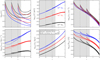 |
Fig. 1 Evolution of the concentration parameter c, the temperature T, the electron density ne, the turbulent velocity υturb, the turbulent driving scale L0, and the equipartition magnetic field Bequ, as a function of the redshift ɀ. Each colour represents a different merger tree configuration with a given mass Mcıust of our modelled cluster at z = 0. The mass resolution is the same in all cases, i.e. Mcıust/Mres = 10−3. Each merger tree mass configuration is also computed for ɀmax = 2-4, where vertical grey dotted lines represent the starting point of the merging process. The solid lines represent the evolution of the plasma quantities without turbulent decay. The coloured dotted lines correspond to the evolution of plasma quantities with turbulent decay according to power laws given by Eqs. (9) and (10). Each line represents, at a given redshift, the skew-normal median of Ntree = 103 merger trees. The grey area corresponds to the part of the merger trees we neglect in the subsequent analysis. |
2.3 Magnetic field strength and vector field
As suggested in Schekochihin & Cowley (2006), Mogavero & Schekochihin (2014), Kunz et al. (2014), Rincon et al. (2016), St-Onge et al. (2020), and Rappaz & Schober (2024), the dynamo in the ICM during the formation of a cluster is explosive, in the sense that the characteristic time associated with the growth rate of the dynamo is extremely short compared to the dynamical time of a cluster. Therefore, we assume that, in the redshift range studied in this work, the magnetic field is always at equipartition with the turbulent velocity field. The equipartition magnetic field is calculated with the (time-dependent) value of υturb as  . Assuming spherical symmetry, the radial distribution of the electron density and magnetic field is interpolated and mapped onto a three-dimensional matrix with the new grid cell size that corresponds to the turbulent forcing scale L0. This implies that the resolution of a box with size (2r200)3 is
  , where we used the default value of the forcing scale L0 = r200 /20. This choice of resolution is motivated by the SSD theory, where the peak of the magnetic energy spectrum moves to smaller wavenumbers after equipartition with the kinetic energy on the dissipative scale is reached. During this non-linear SSD phase, the minimum possible wavenumber that the peak of the magnetic energy spectrum can reach is determined by the inverse of the turbulent forcing scale. However, it should be noted that although it has been suggested that the dynamo of a WCP resembles that of the SSD in classical MHD with high magnetic Prandtl numbers (St-Onge et al. 2020), this tendency has not yet been observed in WCP simulations (see the discussion in Rincon 2019).
In our model, we create a 3D matrix for each component Bi with i = x,y, z of the magnetic field vector as follows. We start by creating a random vector potential A, with the components Ai,i = x,y,z which are generated randomly between −1 and 1. Therefore, the resulting vector F ≡ ∇ × A yields V ⋅ F = 0. In a given numerical cell, if |F| = F, and we set |B| = Bequ, then each component of our 3D magnetic field is Bi ≡ BequFi/F. That way, we obtain three components of a divergence-free vector with an amplitude of Bequ.
2.4 Rotation measure maps
The RM quantifies the rotation of the polarization angle of a linearly polarized wave as it travels through a magnetized medium (Burn 1966; Brentjens & de Bruyn 2005; Ferrière et al. 2021). If .Ψi is the intrinsic polarization angle of the wave, the final angle Ψf after propagating through the magnetized medium is given by
 (12)
(12)
where λ is the observing wavelength, and
 (13)
(13)
with e, me, and c, respectively, denoting the electric charge, the electron mass, and the speed of light. In Eq. (12), ne is the electron density, B|| is the component of the magnetic field vector B parallel to the line of sight, and 𝒟 is the distance from the observer to the source. The quantity RM is called the RM. Then, the RM is numerically computed as
 (14)
(14)
where the sum is performed over all  lines of sight of a given subhalo, and ∆l ≡ 2r200/Nce11 is the size of each cell. Note that the electron density ne has also been mapped onto a 3D matrix, following the equipartition magnetic field. For the rest of this work, we set B|| ≡ Bx. Let us note that every quantity computed in our merger trees is comoving. Therefore, adding the redshift-dependency to Eqs. (13) and (14) means that we are computing the physical RM.
2.5 Averaging processes
Once the radial profiles of the different plasma quantities have been calculated for each MMS in each MT, we average them in two steps to establish a redshift-dependent 1D profile. First, we calculate the root mean square of each quantity Θ in the MMS at a given redshift, as
 (15)
(15)
where Nrad = 103 is the number of grid cells used to create every radial profile. A unique profile is thus obtained for each merger tree. Then, to provide an average estimate of a physical quantity for all merger trees at a given redshift, we follow the same procedure using a skew-normal distribution as described in Appendix C of Rappaz & Schober (2024). In particular, the median value of such a distribution is used as the average estimator. For the rest of this work, such an average is denoted by 〈〉. In Appendix B we discuss the effects of considering other types of averages, like a Gaussian fit or the root mean square. We have established that the different averages considered produce minor variations, and the choice of the averaging process does not impact our conclusions.
Furthermore, Faraday rotation maps are fit with a Gaussian distribution to determine their standard deviation σRM. Finally, we compute radial profiles for the RM (that are compared with radio observations) as follows. We first take the absolute value of a given RM map. Then, we calculate the arithmetic average of every cell located at a given distance r from the cluster centre. The corresponding profile is denoted |µRM(r)|.
3 Results
3.1 Plasma parameters
In this section we present our results on the evolution of different plasma parameters as a function ofredshift. This allows us to determine whether the values obtained for these parameters are similar to those expected from observations, numerical simulations, and other theoretical models. More specifically, the results in this subsection aim to test and ascertain the robustness of our approach.
Figure 1 shows the evolution of different plasma quantities and for different merger tree configurations. The results of the model that assumes turbulent decay are shown as dotted lines. The solid lines correspond to our fiducial turbulent velocity model with L0 = r200/20 and no decay. First, it appears that the turbulent velocity υturb, the driving scale L0, and the equipartition field Bequ vary very little when turbulent decay is considered. Indeed, the most significant disparity between the evolution of Bequ and its decaying counterpart occurs at ɀ ≃ 3.1 for the model with Mc1ust = 1015 M⊙, where the difference between the two curves is approximately a factor 0.8. This difference decreases with the cluster mass. We also note that the decay is more important at the start of the merging process. This can be explained by the increase in major mergers over time (Parkinson et al. 2008). Since the quantities that are affected by turbulent decay only start to decrease from a major merger, the decay becomes less significant when ɀ → 0. Furthermore, the evolution of the various curves at redshifts close to ɀmax is due to our initial conditions and the evolution of the concentration parameter1, which encourages us to focus particularly on the effects occurring at low redshift. Considering this, we can establish that the modelling of turbulent decay laws will not have a significant influence on our conclusions, and are not considered in the rest of this work. Moreover, the parameter ɀmax has minimal influence on the curves as they approach ɀ = 0. Conversely, the trajectories of the various curves in proximity to ɀmax exhibit a similar overall trend. This comes mainly from the evolution of the concentration parameter c, which is similar in models with different ɀmax, as it is displayed in Fig. 1. Indeed, the concentration parameter is calculated by energy conservation between two redshift steps, whether or not a merger occurs. Furthermore, the accretion component is also taken into account in the energy (see Appendix E of Rappaz & Schober 2024). Generally, mass accretion is more important at high redshift, which would explain such a trend.
To ensure methodological rigor, our investigation will focus exclusively on redshift values ranging from 0 to 1.5, mitigating the potential impact of numerical or model artefacts on the results. Additionally, we will exclusively focus on the configuration with ɀmax = 4 to prevent any redundancy in the outcomes.
From Fig. 1, we see that the temperatures obtained at ɀ = 0 for Mclust = 1014 and 1015 M⊙ are approximately between 1.5 and 7 keV. Such values are well in line with the results reported from various X-ray surveys (see e.g. Moretti et al. 2011; Baldi et al. 2012; Wallbank et al. 2022, and references therein). Although our model does not replicate the characteristics of cool-core clusters, the temperatures mentioned above (from our model and observations) are averaged quantities, allowing us to compare them regardless of the dynamic state of the sample of observed clusters.
Also, the typical turbulent velocities from our model are of the order of 150 km s−1 for Mclust = 1014 M⊙ and 300 km s−1 for Mclust = 1015 M⊙. Such values are of the same order of magnitude as the ones derived from X-ray observations of a sample of cool-core clusters obtained by Chandra, as presented in Zhuravleva et al. (2018), which vary between approximately 100 and 150 km s−1. Generally, cool-core clusters are dynamically relaxed. Moreover, sufficient time must elapse after a major merger for the system to reach such a state. It is therefore natural to wonder if our comparison with observations of cool-core clusters is consistent. In fact, in the modified GALFORM model, the major mergers of lower-mass clusters tend to occur at higher redshifts. For Mclust = 1015 M⊙ for instance, the major mergers most often occur at a redshift of ɀ ≃ 0.25. By adopting the same cosmological parameters as those described in Sect. 2.1, this corresponds to approximately 3 Gyr elapsed since the last major merger. This is comparable to the prediction made by Richardson & Corasaniti (2022) for the A2345 cluster, which estimates its last major merger to have occurred approximately 2.2 Gyr ago. Overall, our MT-based models produce results that match low-redshift observations well.
3.2 Rotation measures
In this section we present the results of the RM maps produced in our merger trees. We calculate σRM for regions of varying fixed spatial sizes, as radio observations typically do not encompass the entire cluster and are limited by the coverage of the sources. We also compute the radial profiles of the RM.
3.2.1 RM maps for 1015 M⊙ clusters
Figure 2 shows an example of the RM map calculated for Mclust = 1015 M⊙, for different redshift values. We also show central 2D slices of the 3D distributions of the thermal electron distribution, the turbulent velocity, and the magnetic field component parallel to the line of sight, along which the RM is calculated. In addition, the distributions of the RM are fit with a Gaussian distribution, to illustrate how the standard deviation of the RM, denoted by σRM, is calculated (the mean is ≈0 rad m−2, which is expected of the random magnetic fields in the cluster). The RM distribution computed from the merger tree calculation matches well with a Gaussian distribution, highlighting that the correlation between thermal electron density and magnetic fields (see Fig. C3 in Seta et al. 2023) does not play a significant role (Seta & Federrath 2021a).
For the redshift evolution, we note that the range of RMs and the associated σRM does not evolve significantly (Fig. 2, panel E). This can be explained, in particular, by the evolution of the radial distributions of the thermal electron density ne and the equipartition field Bequ, which are shown in Fig. 3. On one hand, these profiles decrease when ɀ → 0, which is supposed to produce a corresponding decrease in RM magnitude (panel C in the figure). On the other hand, the factor (1 + ɀ)−2 in Eq. (14) attenuates the resulting RM at high redshift, thus decreasing its value. The redshift-diluted RM curves are then much closer together, which explains its very low variation in magnitude over time.
Figure 4 shows the sum along the line of sight of the maps of the electron density, 〈Σne〉 (panel A), the parallel magnetic field component 〈ΣB||〉 (panel B), their product 〈ΣneB||〉 (panel C), and their product divided by (1 + ɀ)2 (panel D), for three different redshift values The maps of all Ntree = 103 MTs are fitted with a skew-normal distribution2, and the median values of these distributions are used to approximate the trend of each curve. It appears that the mean value of the distribution of ΣB|| hardly changes over time, despite the overall decrease of Bequ when z → 0. This is mainly because the magnetic field components are generated randomly, and even re-scaling with the amplitude of Bequ does not generate a significant difference between the distributions. On the other hand, we can see that (Σne) and 〈ΣneB||〉 follow a similar pattern. However, the sum 〈ΣneB||/(1 + ɀ)2〉 seems to have the same tendency as 〈ΣB||〉. Therefore, the evolution of the thermal electron density ne coupled with the (1 + ɀ)−2 factor tends to maintain the observed RM at an approximately constant average value.
3.2.2 Evolution of the RM standard deviation
Figure 5 shows the value of the standard deviation of the RM, denoted σRM, for different MT configurations and redshift values. We consider different characteristic sizes 𝓛 of observed RM patches, which are normalized by the virial radius r200 of the dark matter halos. The reason for conducting such an analysis is that the RM is never observed for the entire structure of a cluster. Radio sources (in the background or inside the cluster) are limited, and the resulting RM patches often have a characteristic size much smaller than that of the observed cluster. It is therefore legitimate to study the trend of σRM as a function of the size of the observed RM maps.
For each value of 𝓛, we extract the submatrix of the corresponding size, centred on each grid cell along the line passing through the centre of the halo. Then, σRM is calculated for all submatrices, which leads to a radial profile σRM = σRM(r, 𝓛). The operation is repeated for each of the Ntree = 103 MTs, and the curves are then averaged by a skew-normal distribution, which tends to smooth out the effect of individual variations for each halo. This can be seen, for example, by comparing Figs. 5 and A.1. Given the spherical symmetry assumed for each halo, performing the same calculations along a different axis is not expected to produce different results.
In our model, 〈σRM〉 is smaller for higher values of ℒ, at least up to ℒ/r200 ≃ 0.4, where all curves seem to match. For example, ℒ/r200 = 0.1 corresponds to a 3 × 3 submatrix, containing only 9 data points. The corresponding distribution is therefore not continuous, and the fitted curve by a Gaussian distribution could be wider, producing a higher standard deviation. We also see that, for Mclust = 1013 and 1014 M⊙, the distributions at different redshifts almost coincide; however, this trend is not the same for Mclust = 1015 M⊙. This can be understood as the effect of the term (1 + ɀ)−2 in Eq. (14) on the average RM magnitude, which will be also discussed in Sect. 3.2.3. Overall, our model predicts that the distribution of 〈σRM〉 is not expected to vary significantly at different redshifts for Mclust ≲ 1014 M⊙. However, we expect 〈σRM〉 to decrease in magnitude as ɀ increases for a characteristic cluster mass somewhere in 1014 M⊙ ≲ Mclust ≲ 1015 M⊙. Establishing this ‘turning-point’ mass would require more values of Mclust to be studied with our merger trees, which can be done in future work.
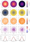 |
Fig. 2 Spatial distribution of characteristic quantities for one realization of a merger tree. The example shows a cluster with Mclust = 1015 M⊙ at ɀ = 0, which has been modelled starting at ɀmax = 4. Each column corresponds to a different value of redshift, as indicated on top. (A) Central 2D slice of the 3D distribution of the electron density. (B) Central 2D slice of the 3D distribution of the turbulent velocity. (C) Central 2D slice of the 3D distribution of the line-of-sight component of the magnetic field. (D) Rotation measure map. (E) Probability distribution function of the RM maps. The red lines correspond to a fit of the histogram data with a Gaussian distribution with the corresponding standard deviation of the Gaussian distribution, σRM, shown in the legend. The mean of the RM distribution is ≈0 rad m−2, as expected for the random magnetic fields. |
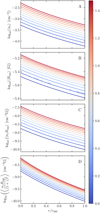 |
Fig. 3 Radial distribution of the electron density (A), the equipartition magnetic field (B), and the product of the two with (D) and without (C) redshift dilution, for Mclust = 1015 M⊙ and ɀmax = 4. Each value at a given radius is the skew-normal median of the values of all Ntree = 103 MTs. We can see that the ne profiles decrease more than that of Bequ. Without redshift dilution, we would expect ne to play a major role in the RM decay. However, because of the (1 + ɀ)−2 factor, RM curves evolve very little over time. |
3.2.3 Averaged RM radial profiles
Figure 6 shows RM radial profiles as a function of the redshift of the cluster for each MT configuration. The shape of the profiles does not appear to change over time. However, for Mclust = 1013 and 1014 M⊙, the profiles are slightly shifted upwards as ɀ increases, but the opposite occurs for Mclust = 1015 M⊙. This effect is illustrated in Fig. 7, which shows the evolution of the value of 〈|µRM|〉 as a function of redshift, for two values of the radius, namely r = 0 and r = r200. There seems to be a mass between Mclust = 1014 and 1015 M⊙ for which the trend reverses. As shown in Fig. 1, the evolution of Bequ is faster for Mclust = 1013 M⊙ than for the other configurations. By associating this with the wavelength dilution given by the factor (1 + ɀ)−2 in Eq. (13), as well as the fact that the average RM increases with the mass of the clusters, this trend can be explained. Moreover, the evolution of the equipartition magnetic field is intrinsically linked to the evolution of the turbulent velocity field, which in our case is a simplified model. Therefore, there is a possibility that this effect does not originate from any underlying physical mechanism, but rather from a characteristic inherent to our model. Testing this hypothesis would require observational data from multiple radio sources in clusters up to ɀ = 1.5, unavailable today. However, this may prove possible with the next generation of radio telescopes, such as the Square Kilometre Array (Heald et al. 2020).
The profiles in Fig. 6 were fitted with a function of the form
 (16)
(16)
where γ and . are fitting parameters. The optimal values of γ are presented in Fig. 8. Notably, for configurations with Mclust = 1014 and 1015 M⊙, there is a marginal decrease in the curves as ɀ → 0, but these variations are negligible. Consequently, it is reasonable to assert that the slope of these profiles remains constant within the examined redshift range. Conversely, for Mclust = 1013 M⊙, a more substantial temporal variation is observed. Nevertheless, this variation is minor, ranging from approximately γ ≃−1.5 at ɀ = 1.5 to around γ ≃−1.38 at ɀ = 0. However, the discernible difference in trend among these curves cannot definitively be attributed to a specific physical mechanism or potential numerical effects intrinsic to our methods.
3.3 Comparison with radio observations
In this section we compare the RM radial distribution obtained with our model at ɀ = 0 to various radio observations, to test the robustness of our approach. We selected a sample of radio observations of various clusters with masses between ~1014 and 5 × 10¹⁵ M⊙ and redshifts between ɀ ≃ 0.0140 and ɀ ≃ 0.0801. The RM data are retrieved from Bonafede et al. (2010) for A1656, from Govoni et al. (2010) for A119, A514 and A225, and from Clarke et al. (2001) for A376, A426, A496, A754, A1060, A1314 and A2247. Relevant data concerning virial mass, virial radius r200, and redshift were obtained from survey catalogues (Girardi et al. 1998; Abell et al. 1989; Groener et al. 2016, and references therein). Additionally, we also included radio analyses for A2255 from Govoni et al. (2005), and for A400 and A2634 from Eilek & Owen (2002). The observed values of the RM correspond to the mean of the normal distribution used to fit the observational data, and the error (when available) corresponds to the standard deviation of the distribution.
The comparison of our model with such observations is shown in the left-hand panel of Fig. 9. The solid lines correspond to the radial profiles of our model at ɀ = 0 for the three MT configurations. The colours indicate the observed cluster mass or the value Mclust in our model, respectively. The black markers indicate radio observations for clusters whose mass has not been estimated. Despite obvious variations between our model and the reported observational values due to many factors discussed in the next section, the overall trend of the RM as a function of radius appears to be in good agreement with observations for .clust = lO15 .⊙, which is an encouraging indication of the robustness of our approach. It should be noted, however, that our model and the observational data do not represent the same entities. The curves in our model represent the average of all RM values at a given radius. The observational data points reported represent the average RM value observed for a radio source with a certain spatial extent, at a given distance from the cluster’s centre.
We also compared our model with the detailed observational data of a low-mass and low-redshift cluster, namely Abell S0373 (Fornax). The polarimetric data of Fornax sources are retrieved from Anderson et al. (2021). We compute the projected angular distance from NGC 1399 (considered in the original paper as the centre of the cluster) assuming that the galaxy is located at a distance of 20.24 Mpc (e.g. Lavaux & Hudson 2011). Fornax’s virial radius is assumed to be r200 = 0.7 Mpc, its redshift ɀ = 0.005 and its mass M = 6 × 10¹³ .⊙ (e.g. Maddox et al. 2019; Anderson et al. 2021, and references therein.). The results are shown in the middle panel of Fig. 9 respectively. We have plotted the curves corresponding to our model at ɀ = 0 (solid lines). The Fornax data were fitted with a function proportional to  where α is a real number, which corresponds to the black dotted line in Fig. 9. It appears that our model with Mclust = 1014 M⊙ and the observations from Anderson et al. (2021) are in relatively good agreement up to about r/r200 ≃ 0.4, and for α ≃−0.118 ± 0.022. However, the RM profile of our model decreases, while the Fornax profile seems to be almost constant with r. However, Fornax is supposed to be in an ongoing merger with the Fornax A substructure, which tends to make the assumption of spherical symmetry of the baryonic gas inapplicable for this cluster. Nevertheless, the good match between the central region of Fornax and our model is an encouraging sign of the robustness of our approach and seems to confirm that lower-mass clusters produce weaker RM signals than their more massive counterparts.
Finally, we also compared our model with the observational data of a massive, high-redshift cluster, namely Abell 2345. Its various data are retrieved from Stuardi et al. (2021). Its redshift is reported as ɀ = 0.1789, its mass as M = 2.85 × 10¹⁵ M⊙. and its virial radius as r200 = 3.4 Mpc (all comoving, see e.g. Boschin et al. 2010). The results are shown on the right panel of Fig. 9. We have plotted the curves corresponding to our model at ɀ = 0.174 (dashed lines), which is the closest redshift of our model to that of Abell 2345. Its central part also seems to be in good agreement with our results. Similarly, this cluster presents two non-symmetric radio relics, and Boschin et al. (2010) have suggested that it is undergoing a merger, making its matter distribution highly asymmetric as well, which tends to explain the discrepancies observed at r/r200 ≃ 0.4. It should also be noted that the higher redshift value of Abell 2345 does not alter our predictions regarding its RM values, as shown by the various curves of our model in the right-hand panel of Fig. 9. In addition, several obvious aspects that could change our results are discussed in Sect. 4.
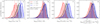 |
Fig. 4 Average distribution of the sum along the line of sight (x-axis) of the electron density (A), the parallel component of the magnetic field (B). the product of those two quantities (C), and the product divided by the (1 +z)−2 contribution, for Ntree = 103 MTs of our model with Mclust = 1015M⊙. In the same panel, each distribution corresponds to a given redshift value. Each histogram is fitted with a skew-normal distribution (see Appendix C of Rappaz & Schober 2024) which is shown in solid lines and the median value of the latter is displayed in dotted lines, to highlight which parameter amongst the electron density and the line-of-sight component of the magnetic field has the most influence on the rotation measure. It appears that if the contribution of the expansion of the universe is not taken into account, the distribution of thermal electron density is dominant. With the expansion, the RM shows minor variations. |
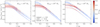 |
Fig. 5 Evolution of the standard deviation σRM of the RM computed for the equipartition magnetic field Bequ as a function of the redshift. Each column corresponds to a specific MT configuration. The different colours correspond to the ratio of the typical size ℒ of the observed RM patch to the virial radius of the halo. Note that the profiles are calculated up to the value of r where the edge of the extracted sub-matrix with a size corresponding to a given value of ℒ/r200 reaches r200. Therefore, for higher values of ℒ/r200 the profiles extend up to lower values of r/r200. |
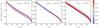 |
Fig. 6 Radial-averaged RM of the equipartition magnetic field Bequ as a function of the radius normalized to r200, for the three MT configurations. Each coloured line corresponds to a given redshift value, up to ɀ = 1.5. |
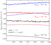 |
Fig. 7 Evolution of 〈|μRM.〉 at r = 0 (solid lines) and r = r200/2 (dashed lines), as a function of the redshift, for the three MT configurations. |
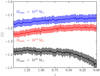 |
Fig. 8 Best-fit values for the fitting parameter γ in Eq. (16). The solid lines represent the skew-normal median of γ of all MTs at a given redshift. The shaded areas are the errors given by the skew-normal standard deviation. |
4 Discussion
4.1 Missing physics
The advantage of our model is its simplicity which allows us to scan a large range of characteristic parameters of galaxy clusters. However, our model is relatively basic, and several factors might influence our results. Firstly, our assumptions of spherical symmetry and the nature of plasma are rough. Although we aim to study global RM trends, it is well known that the ICM is multiphase. For instance, observations have shown the presence of regions of cold neutral hydrogen gas, calling into question the dominant character of hot gas in the ICM (Bonamente et al. 2001). The effect of the multiphase nature of the ICM on X-ray observables was investigated using data from hydrodynamic simulations, including components such as AGN feedback (ZuHone et al. 2023). Furthermore, from recent turbulent magnetohydro-dynamic simulations, it is known that the multiphase nature of the medium affects magnetic field properties (Seta & Federrath 2022; Mohapatra et al. 2022; Das & Gronke 2024). We also adopted a very simple turbulent velocity model, assuming that turbulence was only generated by shocks and shear from mergers of dark matter halos. However, recent 3D MHD simulations have shown, for example, that turbulence in the ICM hot gas could also have contributions from AGN jets or the stream of precipitating cold filaments (Wang et al. 2021).
Finally, we assume that the SSD amplifies the magnetic field up to equipartition with the turbulent velocity field and that the magnetic energy peak shifts towards larger spatial scales in the nonlinear dynamo phase. At saturation, we assume that the peak of the magnetic energy spectrum has reached the turbulent forcing scale. While such a shift of magnetic energy towards larger scales is observed in numerical simulations (e.g. Federrath et al. 2014; Seta & Federrath 2021b), it remains unclear whether this shift continues up to the forcing scale. Moreover, this is even less known and understood for weakly collisional plasmas.
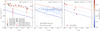 |
Fig. 9 Comparison of the predicted RM radial profiles from our model with radio observations. (Left) Comparison of the modelled RM radial profiles with the following observational data from radio sources of a sample of various clusters: A1656 (Coma) from Bonafede et al. (2010); A2255, A119, and A514 from Govoni et al. (2010); A376, A426 (Perseus), A496, A754, A1060 (Hydra), A1314, and A2247 from Clarke et al. (2001); A2255 from Govoni et al. (2005); and A400 and A2634 from Eilek & Owen (2002). Our model with Mclust = 1015 M⊙ seems to be in good agreement with the observations. In particular, a strong similarity is observed with observations of A1656 (Coma), probably due to its high X-ray emission symmetry. Significant deviations are observed for A1060 (Hydra) and A426 (Perseus), probably due to high AGN activity and strong gas mixing. (Centre) Comparison of our RM model with the galactic foreground corrected data of the AS0373 (Fornax) cluster from Anderson et al. (2021). The solid lines correspond to our model at ɀ = 0. The black dotted line corresponds to a fit of the form |

4.2 Possible observational effects
We have seen that our predictions for the RM are in good agreement with observations of multiple radio sources in a set of about ten clusters. However, several factors could bias our results. Our RM maps are calculated on the assumption that each numerical cell is a source of linearly polarized wave emission. In this case, the redshift of the source corresponds to the redshift of the cluster studied. Depending on the redshift of the emitting source, this may, for example, cause a vertical shift in the observations. The effect of intracluster sources is also not analysed, nor is the emission of cosmic ray electrons from the ICM. However, in observations presented in Bonafede et al. (2010) some radio sources are located within the virial radius of the cluster. Also, it is common for several distinctive areas of RM emission to originate from the same radio source. Depending on the reverse scale of the ICM’s magnetic field, some of these zones may thus present different values, sometimes of opposite sign, producing a discontinuous RM distribution (e.g. Govoni et al. 2010; Bonafede et al. 2010). Averaging such data using a Gaussian fit could produce a different standard deviation value from that observed if more data were available. More generally, the cosmic ray and thermal electrons in the ICM are mixed and thus the emission and Faraday rotation of the emission happens within the same region. This might affect some of our results, especially the estimates of σRM. We also assumed that the resolution of our RM maps was set by the turbulent driving scale, as the SSD predicts that the power spectrum of magnetic energy shifts towards such length scales from the moment the magnetic energy density is more or less in equipartition with the kinetic energy density of the turbulence. However, the non-linear effects of dynamo in WCPs have yet to be fully elucidated. Thus, if the typical length scale of the magnetic field were to vary spatially, the results could differ from our predictions.
5 Conclusions
Magnetic fields in the microgauss range are systematically observed in the ICM of galaxy clusters. The previous work by Rappaz & Schober (2024), which was motivated by the pioneering work of Schekochihin & Cowley (2006), St-Onge & Kunz (2018), and St-Onge et al. (2020), suggests that if such fields were amplified from primordial fields, the growth of the magnetized field would be much faster than suggested by classical MHD theory. In this paper, we study the evolution of the RM implemented in MTs generated by the modified GALFORM algorithm (Parkinson et al. 2008), assuming that the magnetic field had already been amplified to equipartition with the turbulent velocity field. The main outcomes of this work are the following.
The average RM is the highest for our MT configuration with Mclust = 1015 .⊙, and the lowest with Mclust = 1013 .⊙. In all MT configurations, the mean RM amplitude does not change significantly up to redshift ɀ ≃ 1.5. This effect is due to two contributions. Between ɀmax ≃ 1.5 and ɀ = 0, the mean thermal electron density ne decreases, which causes the RM to be higher at ɀmax. At the same time, the RM depends on the redshift as (1 + ɀ)−2. The two effects compensate for each other, resulting in no major evolution in the RM. For Mclust = 1014 and 1015 M⊙. the RM radial profiles μRM follow approximately the same power law, that is, log10(µRM) ∝ −1.2(r/r200). For Mclust = 1013 M⊙. this relation is log10.µRM. ∝ − 1.4(r/r200). Overall, the radial profile associated with our model with Mclust = 1015 M⊙ to ɀ = 0 is in good agreement with radio observations from various clusters. The observations of Abell1656 (Coma) are the closest to our model. We assume that the main reason for such a good agreement is that Coma has recently (approximately 1 Gyr ago) undergone a major merger event with the NGC 4839 group, and is now settling in a configuration close to hydrostatic equilibrium, as suggested by Neumann et al. (2003) and Churazov et al. (2021). This gives it a symmetry in X-ray emission that is very close to our assumption of spherical symmetry for the plasma quantities implemented in our subhalos. On the other hand, our model does not agree well with certain values of the Abell426 (Perseus) observations. We assume that this is due to strong AGN activity in Perseus’ core and in particular an X-ray emission structure suggestive of strong gas mixing (see e.g. Zhuravleva et al. 2014).
Our model does not include certain factors likely to modify the observed RM value, such as AGN jets, the multiphase nature of the ICM, and sources of turbulence besides merging halos. Despite this, we suggest that our model can be used to efficiently create radial RM distributions for redshifts up to ɀ ≃ 1.5, for clusters with masses of the order of 1015 M⊙. The complete analysis, from the raw data of the modified GALFORM to the results presented in this work, does indeed take just one or two days, on a set of around ten conventional CPUs. This is very time-saving compared with full-scale MHD cosmological simulations, which can take several months or even years to complete and process. Finally, our model could prove useful in the creation of mock radio observations for next-generation radio telescopes, such as the Square Kilometre Array (Heald et al. 2020).
Acknowledgements
We are grateful to Jean-Paul Kneib, Antoine Rocher, and Aurélien Verdier for very useful discussions on the cosmology part of this work. We thank Radhika Achikanath Chirakkara for useful discussions related to dynamos in galaxy clusters. Y.R. and J.S. acknowledge the support from the Swiss National Science Foundation under Grant No. 185863. C.F. acknowledges funding provided by the Australian Research Council (Discovery Project DP230102280), and the Australia-Germany Joint Research Cooperation Scheme (UA-DAAD).
Appendix A RM maps resolution
In this section we study the effect of both numerical resolution and forcing scale values on the computed signals of the RM. Figure A.1 shows the effect of increasing the resolution in each grid cell of an RM map by a factor Λ on the radial profile of the RM and its standard deviation. In particular, the profiles are computed for a single realization of a merger tree with Mclust = 1015 M⊙, at ɀ = 0. For σRM, we compute the profiles for ℒ/r200 = 0.2 and 0.5. Overall, there is no difference between the curves, and we directly conclude that Λ does not affect the final result.
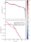 |
Fig. A.1 Effect of increasing the resolution in each grid cell of an RM map by a factor of Λ, on the radial profile of the RM (top) and its standard deviation (bottom). The different curves are calculated for a single tree with Mclust = 1015 M⊙. |
Appendix B Effect of different averages
Here, we present an analysis of the effect of different types of averages on the evolution of the temperature, for our model with Mclust = 1015 M⊙. To do this, we calculated the temperature profile for each Ntree = 103 MTs. At each fixed red-shift value, we estimated the mean of the temperature values of all MTs in different ways. Specifically, we calculated the arithmetic mean 〈T〉, the root mean square 〈T〉rms, the median value 〈T〉SN of the fit of the data with a skew-normal distribution, as well as the mean 〈T〉gauss of the fit of the data with a normal distribution. We then repeated the same operation but on logarithmic temperature values. Figure B.1 shows the different results of such averaging processes on temperature evolution. It is clear that the variations between averages are minor, and that the arbitrary choice of one of these processes does not change the results and conclusions of our study.
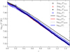 |
Fig. B.1 Evolution of the temperature T for Mclust = 1015 M⊙ and ɀmax calculated in different ways. The lines correspond to the arithmetic mean 〈〉a, the root-mean-square 〈〉rms, the median of a skew-normal fitting 〈〉, and the average of a Gaussian fitting 〈〉gauss, for which the logarithm was taken. The markers correspond to the same average processes but are performed on the logarithmic values of T. |
References
- Abell, G. O., Corwin, J., Harold G., & Olowin, R. P. 1989, ApJS, 70, 1 [NASA ADS] [CrossRef] [Google Scholar]
- Achikanath Chirakkara, R., Seta, A., Federrath, C., & Kunz, M. W. 2024, MNRAS, 528, 937 [NASA ADS] [CrossRef] [Google Scholar]
- Anderson, C. S., Heald, G. H., Eilek, J. A., et al. 2021, PASA, 3 8, e020 [CrossRef] [Google Scholar]
- Baldi, A., Ettori, S., Molendi, S., & Gastaldello, F. 2012, A&A, 545, A41 [NASA ADS] [CrossRef] [EDP Sciences] [Google Scholar]
- Bhat, P., & Subramanian, K. 2013, MNRAS, 429, 2469 [NASA ADS] [CrossRef] [Google Scholar]
- Bonafede, A., Feretti, L., Murgia, M., et al. 2010, A&A, 513, A30 [NASA ADS] [CrossRef] [EDP Sciences] [Google Scholar]
- Bonamente, M., Lieu, R., & Mittaz, J. P. D. 2001, ApJ, 546, 805 [NASA ADS] [CrossRef] [Google Scholar]
- Boschin, W., Barrena, R., & Girardi, M. 2010, A&A, 521, A78 [NASA ADS] [CrossRef] [EDP Sciences] [Google Scholar]
- Braginskii, S. I. 1965, Rev. Plasma Phys., 1, 205 [Google Scholar]
- Brandenburg, A., & Subramanian, K. 2005, Phys. Rep., 417, 1 [NASA ADS] [CrossRef] [Google Scholar]
- Brandenburg, A., Rogachevskii, I., & Schober, J. 2023, MNRAS, 518, 6367 [Google Scholar]
- Brentjens, M. A., & de Bruyn, A. G. 2005, A&A, 441, 1217 [NASA ADS] [CrossRef] [EDP Sciences] [Google Scholar]
- Burn, B. J. 1966, MNRAS, 133, 67 [Google Scholar]
- Chandrasekhar, S., Kaufman, A. N., & Watson, K. M. 1958, Proc. R. Soc. London Ser. A, 245, 435 [NASA ADS] [CrossRef] [Google Scholar]
- Cho, J. 2014, ApJ, 797, 133 [NASA ADS] [CrossRef] [Google Scholar]
- Churazov, E., Khabibullin, I., Lyskova, N., Sunyaev, R., & Bykov, A. M. 2021, A&A, 651, A41 [NASA ADS] [CrossRef] [EDP Sciences] [Google Scholar]
- Clarke, T. E., Kronberg, P. P., & Böhringer, H. 2001, ApJ, 547, L111 [NASA ADS] [CrossRef] [Google Scholar]
- Cole, S., Lacey, C. G., Baugh, C. M., & Frenk, C. S. 2000, MNRAS, 319, 168 [Google Scholar]
- Das, H. K., & Gronke, M. 2024, MNRAS, 527, 991 [Google Scholar]
- Di Gennaro, G., van Weeren, R. J., Brunetti, G., et al. 2021, Nat. Astron., 5, 268 [Google Scholar]
- Donnert, J., Dolag, K., Lesch, H., & Müller, E. 2009, MNRAS, 392, 1008 [NASA ADS] [CrossRef] [Google Scholar]
- Donnert, J., Vazza, F., Brüggen, M., & ZuHone, J. 2018, Space Sci. Rev., 214, 122 [Google Scholar]
- Dvorkin, I., & Rephaeli, Y. 2011, MNRAS, 412, 665 [NASA ADS] [CrossRef] [Google Scholar]
- Eilek, J. A., & Owen, F. N. 2002, ApJ, 567, 202 [NASA ADS] [CrossRef] [Google Scholar]
- Enßlin, T. A., & Vogt, C. 2003, A&A, 401, 835 [NASA ADS] [CrossRef] [EDP Sciences] [Google Scholar]
- Federrath, C. 2016, J. Plasma Phys., 82, 535820601 [Google Scholar]
- Federrath, C., Roman-Duval, J., Klessen, R. S., Schmidt, W., & Mac Low, M. M. 2010, A&A, 512, A81 [NASA ADS] [CrossRef] [EDP Sciences] [Google Scholar]
- Federrath, C., Schober, J., Bovino, S., & Schleicher, D. R. G. 2014, ApJ, 797, L19 [NASA ADS] [CrossRef] [Google Scholar]
- Federrath, C., Klessen, R. S., Iapichino, L., & Beattie, J. R. 2021, Nat. Astron., 5, 365 [NASA ADS] [CrossRef] [Google Scholar]
- Ferrière, K., West, J. L., & Jaffe, T. R. 2021, MNRAS, 507, 4968 [Google Scholar]
- Gary, S. P. 1992, J. Geophys. Res., 97, 8519 [NASA ADS] [CrossRef] [Google Scholar]
- Girardi, M., Giuricin, G., Mardirossian, F., Mezzetti, M., & Boschin, W. 1998, ApJ, 505, 74 [NASA ADS] [CrossRef] [Google Scholar]
- Govoni, F., Murgia, M., Feretti, L., et al. 2005, A&A, 430, L5 [NASA ADS] [CrossRef] [EDP Sciences] [Google Scholar]
- Govoni, F., Dolag, K., Murgia, M., et al. 2010, A&A, 522, A105 [NASA ADS] [CrossRef] [EDP Sciences] [Google Scholar]
- Groener, A. M., Goldberg, D. M., & Sereno, M. 2016, MNRAS, 455, 892 [NASA ADS] [CrossRef] [Google Scholar]
- Haugen, N. E., Brandenburg, A., & Dobler, W. 2004, Phys. Rev. E, 70, 016308 [NASA ADS] [CrossRef] [Google Scholar]
- Heald, G., Mao, S. A., Vacca, V., et al. 2020, Galaxies, 8, 53 [NASA ADS] [CrossRef] [Google Scholar]
- Hellinger, P. 2007, Phys. Plasmas, 14, 082105 [NASA ADS] [CrossRef] [Google Scholar]
- Jiang, F., & van den Bosch, F. C. 2014, MNRAS, 440, 193 [CrossRef] [Google Scholar]
- Kim, K. T., Tribble, P. C., & Kronberg, P. P. 1991, ApJ, 379, 80 [NASA ADS] [CrossRef] [Google Scholar]
- Kravtsov, A. V., & Borgani, S. 2012, ARA&A, 50, 353 [Google Scholar]
- Kriel, N., Beattie, J. R., Seta, A., & Federrath, C. 2022, MNRAS, 513, 2457 [NASA ADS] [CrossRef] [Google Scholar]
- Kritsuk, A. G., Norman, M. L., Padoan, P., & Wagner, R. 2007, ApJ, 665, 416 [NASA ADS] [CrossRef] [Google Scholar]
- Kuchar, P., & Enßlin, T.A. 2011, A&A, 529, A13 [NASA ADS] [CrossRef] [EDP Sciences] [Google Scholar]
- Kulsrud, R. M. 1983, in Handbook of Plasma Physics, Basic plasma physics I., eds. A. A. Galeev, & R. N. Sudan (Amsterdam: North-Holland Publishing Company), 1115 [Google Scholar]
- Kunz, M. W., Schekochihin, A. A., & Stone, J. M. 2014, Phys. Rev. Lett., 112, 205003 [NASA ADS] [CrossRef] [Google Scholar]
- Lavaux, G., & Hudson, M. J. 2011, MNRAS, 416, 2840 [Google Scholar]
- Maddox, N., Serra, P., Venhola, A., et al. 2019, MNRAS, 490, 1666 [Google Scholar]
- Malvadi Shivakumar, L., & Federrath, C. 2023, arXiv e-prints [arXiv:2311.10350] [Google Scholar]
- Marinacci, F., Vogelsberger, M., Pakmor, R., et al. 2018, MNRAS, 480, 5113 [NASA ADS] [Google Scholar]
- Melville, S., Schekochihin, A. A., & Kunz, M. W. 2016, MNRAS, 459, 2701 [NASA ADS] [CrossRef] [Google Scholar]
- Mogavero, F., & Schekochihin, A. A. 2014, MNRAS, 440, 3226 [NASA ADS] [CrossRef] [Google Scholar]
- Mohapatra, R., Jetti, M., Sharma, P., & Federrath, C. 2022, MNRAS, 510, 3778 [NASA ADS] [CrossRef] [Google Scholar]
- Moretti, A., Gastaldello, F., Ettori, S., & Molendi, S. 2011, A&A, 528, A102 [NASA ADS] [CrossRef] [EDP Sciences] [Google Scholar]
- Navarro, J. F., Frenk, C. S., & White, S. D. M. 1996, ApJ, 462, 563 [Google Scholar]
- Nelson, D., Pillepich, A., Springel, V., et al. 2019, MNRAS, 490, 3234 [Google Scholar]
- Neumann, D. M., Lumb, D. H., Pratt, G. W., & Briel, U. G. 2003, A&A, 400, 811 [NASA ADS] [CrossRef] [EDP Sciences] [Google Scholar]
- Ostriker, J. P., Bode, P., & Babul, A. 2005, ApJ, 634, 964 [NASA ADS] [CrossRef] [Google Scholar]
- Parker, E. N. 1958, Phys. Rev., 109, 1874 [NASA ADS] [CrossRef] [Google Scholar]
- Parkinson, H., Cole, S., & Helly, J. 2008, MNRAS, 383, 557 [Google Scholar]
- Planck Collaboration VI. 2020, A&A, 641, A6 [NASA ADS] [CrossRef] [EDP Sciences] [Google Scholar]
- Press, W. H., & Schechter, P. 1974, ApJ, 187, 425 [Google Scholar]
- Rappaz, Y., & Schober, J. 2024, A&A, 683, A35 [NASA ADS] [CrossRef] [EDP Sciences] [Google Scholar]
- Richardson, T. R. G., & Corasaniti, P. S. 2022, MNRAS, 513, 4951 [NASA ADS] [CrossRef] [Google Scholar]
- Rincon, F. 2019, J. Plasma Phys., 85, 205850401 [NASA ADS] [CrossRef] [Google Scholar]
- Rincon, F., Schekochihin, A. A., & Cowley, S. C. 2015, MNRAS, 447, L45 [NASA ADS] [CrossRef] [Google Scholar]
- Rincon, F., Califano, F., Schekochihin, A. A., & Valentini, F. 2016, Proc. Natl. Acad. Sci., 113, 3950 [NASA ADS] [CrossRef] [Google Scholar]
- Rudakov, L. I., & Sagdeev, R. Z. 1961, Sov. Phys. Doklady, 6, 415 [NASA ADS] [Google Scholar]
- Santos-Lima, R., de Gouveia Dal Pino, E. M., Kowal, G., et al. 2014, ApJ, 781, 84 [NASA ADS] [CrossRef] [Google Scholar]
- Schekochihin, A. A., & Cowley, S. C. 2006, Phys. Plasmas, 13, 056501 [NASA ADS] [CrossRef] [Google Scholar]
- Schekochihin, A. A., Cowley, S. C., Taylor, S. F., Maron, J. L., & McWilliams, J. C. 2004, ApJ, 612, 276 [NASA ADS] [CrossRef] [Google Scholar]
- Schekochihin, A. A., Cowley, S. C., Rincon, F., & Rosin, M. S. 2010, MNRAS, 405, 291 [NASA ADS] [Google Scholar]
- Schober, J., Schleicher, D., Federrath, C., Klessen, R., & Banerjee, R. 2012, Phys. Rev. E, 85, 026303 [NASA ADS] [CrossRef] [Google Scholar]
- Schober, J., Schleicher, D. R. G., & Klessen, R. S. 2013, A&A, 560, A87 [NASA ADS] [CrossRef] [EDP Sciences] [Google Scholar]
- Seta, A., & Federrath, C. 2020, MNRAS, 499, 2076 [NASA ADS] [CrossRef] [Google Scholar]
- Seta, A., & Federrath, C. 2021a, MNRAS, 502, 2220 [NASA ADS] [CrossRef] [Google Scholar]
- Seta, A., & Federrath, C. 2021b, Phys. Rev. Fluids, 6, 103701 [NASA ADS] [CrossRef] [Google Scholar]
- Seta, A., & Federrath, C. 2022, MNRAS, 514, 957 [NASA ADS] [CrossRef] [Google Scholar]
- Seta, A., Bushby, P. J., Shukurov, A., & Wood, T. S. 2020, Phys. Rev. Fluids, 5, 043702 [NASA ADS] [CrossRef] [Google Scholar]
- Seta, A., Federrath, C., Livingston, J. D., & McClure-Griffiths, N. M. 2023, MNRAS, 518, 919 [Google Scholar]
- Shi, X., Nagai, D., & Lau, E. T. 2018, MNRAS, 481, 1075 [NASA ADS] [CrossRef] [Google Scholar]
- Southwood, D. J., & Kivelson, M. G. 1993, J. Geophys. Res., 98, 9181 [NASA ADS] [CrossRef] [Google Scholar]
- Springel, V., White, S. D. M., Jenkins, A., et al. 2005, Nature, 435, 629 [Google Scholar]
- St-Onge, D. A., & Kunz, M. W. 2018, ApJ, 863, L25 [CrossRef] [Google Scholar]
- St-Onge, D. A., Kunz, M. W., Squire, J., & Schekochihin, A. A. 2020, J. Plasma Phys., 86, 905860503 [NASA ADS] [CrossRef] [Google Scholar]
- Stasyszyn, F. A., & de los Rios, M. 2019, MNRAS, 487, 4768 [NASA ADS] [CrossRef] [Google Scholar]
- Stuardi, C., Bonafede, A., Lovisari, L., et al. 2021, MNRAS, 502, 2518 [NASA ADS] [CrossRef] [Google Scholar]
- Subramanian, K., Shukurov, A., & Haugen, N. E. L. 2006, MNRAS, 366, 1437 [CrossRef] [Google Scholar]
- Sur, S. 2019, MNRAS, 488, 3439 [NASA ADS] [CrossRef] [Google Scholar]
- Vazza, F., Roediger, E., & Brüggen, M. 2012, A&A, 544, A103 [NASA ADS] [CrossRef] [EDP Sciences] [Google Scholar]
- Vazza, F., Brüggen, M., Gheller, C., & Wang, P. 2014, MNRAS, 445, 3706 [CrossRef] [Google Scholar]
- Wallbank, A. N., Maughan, B. J., Gastaldello, F., Potter, C., & Wik, D. R. 2022, MNRAS, 517, 5594 [NASA ADS] [CrossRef] [Google Scholar]
- Wang, C., Ruszkowski, M., Pfrommer, C., Oh, S. P., & Yang, H. Y. K. 2021, MNRAS, 504, 898 [NASA ADS] [CrossRef] [Google Scholar]
- Zhuravleva, I., Churazov, E., Schekochihin, A. A., et al. 2014, Nature, 515, 85 [Google Scholar]
- Zhuravleva, I., Allen, S. W., Mantz, A., & Werner, N. 2018, ApJ, 865, 53 [CrossRef] [Google Scholar]
- ZuHone, J., Bahar, Y. E., Biffi, V., et al. 2023, A&A, 675, A150 [NASA ADS] [CrossRef] [EDP Sciences] [Google Scholar]
More precisely, we mentioned in Sect. 2.1 that c is calculated by energy conservation before and after a merger. When a halo does not participate in any merger, as is often the case for redshifts close to ɀmax, only the energy component of the accreted matter is added to the halo’s energy, decreasing the value of c. On the other hand, as ɀ approaches zero, more mergers take place, and the value of c increases. The evolution of gas density ρg (and therefore of ne) then follows a similar trend. Subsequently, as all other plasma quantities are calculated as a function of ne, T, and υturb, they also follow a similar trend.
Taking the sum of the different quantities along the x-axis leads to a distribution closer to a skew-normal distribution. This is why we choose not to fit the distributions with a Gaussian law.
All Figures
|
Fig. 1 Evolution of the concentration parameter c, the temperature T, the electron density ne, the turbulent velocity υturb, the turbulent driving scale L0, and the equipartition magnetic field Bequ, as a function of the redshift ɀ. Each colour represents a different merger tree configuration with a given mass Mcıust of our modelled cluster at z = 0. The mass resolution is the same in all cases, i.e. Mcıust/Mres = 10−3. Each merger tree mass configuration is also computed for ɀmax = 2-4, where vertical grey dotted lines represent the starting point of the merging process. The solid lines represent the evolution of the plasma quantities without turbulent decay. The coloured dotted lines correspond to the evolution of plasma quantities with turbulent decay according to power laws given by Eqs. (9) and (10). Each line represents, at a given redshift, the skew-normal median of Ntree = 103 merger trees. The grey area corresponds to the part of the merger trees we neglect in the subsequent analysis. |
| In the text | |
|
Fig. 2 Spatial distribution of characteristic quantities for one realization of a merger tree. The example shows a cluster with Mclust = 1015 M⊙ at ɀ = 0, which has been modelled starting at ɀmax = 4. Each column corresponds to a different value of redshift, as indicated on top. (A) Central 2D slice of the 3D distribution of the electron density. (B) Central 2D slice of the 3D distribution of the turbulent velocity. (C) Central 2D slice of the 3D distribution of the line-of-sight component of the magnetic field. (D) Rotation measure map. (E) Probability distribution function of the RM maps. The red lines correspond to a fit of the histogram data with a Gaussian distribution with the corresponding standard deviation of the Gaussian distribution, σRM, shown in the legend. The mean of the RM distribution is ≈0 rad m−2, as expected for the random magnetic fields. |
| In the text | |
|
Fig. 3 Radial distribution of the electron density (A), the equipartition magnetic field (B), and the product of the two with (D) and without (C) redshift dilution, for Mclust = 1015 M⊙ and ɀmax = 4. Each value at a given radius is the skew-normal median of the values of all Ntree = 103 MTs. We can see that the ne profiles decrease more than that of Bequ. Without redshift dilution, we would expect ne to play a major role in the RM decay. However, because of the (1 + ɀ)−2 factor, RM curves evolve very little over time. |
| In the text | |
|
Fig. 4 Average distribution of the sum along the line of sight (x-axis) of the electron density (A), the parallel component of the magnetic field (B). the product of those two quantities (C), and the product divided by the (1 +z)−2 contribution, for Ntree = 103 MTs of our model with Mclust = 1015M⊙. In the same panel, each distribution corresponds to a given redshift value. Each histogram is fitted with a skew-normal distribution (see Appendix C of Rappaz & Schober 2024) which is shown in solid lines and the median value of the latter is displayed in dotted lines, to highlight which parameter amongst the electron density and the line-of-sight component of the magnetic field has the most influence on the rotation measure. It appears that if the contribution of the expansion of the universe is not taken into account, the distribution of thermal electron density is dominant. With the expansion, the RM shows minor variations. |
| In the text | |
|
Fig. 5 Evolution of the standard deviation σRM of the RM computed for the equipartition magnetic field Bequ as a function of the redshift. Each column corresponds to a specific MT configuration. The different colours correspond to the ratio of the typical size ℒ of the observed RM patch to the virial radius of the halo. Note that the profiles are calculated up to the value of r where the edge of the extracted sub-matrix with a size corresponding to a given value of ℒ/r200 reaches r200. Therefore, for higher values of ℒ/r200 the profiles extend up to lower values of r/r200. |
| In the text | |
|
Fig. 6 Radial-averaged RM of the equipartition magnetic field Bequ as a function of the radius normalized to r200, for the three MT configurations. Each coloured line corresponds to a given redshift value, up to ɀ = 1.5. |
| In the text | |
|
Fig. 7 Evolution of 〈|μRM.〉 at r = 0 (solid lines) and r = r200/2 (dashed lines), as a function of the redshift, for the three MT configurations. |
| In the text | |
|
Fig. 8 Best-fit values for the fitting parameter γ in Eq. (16). The solid lines represent the skew-normal median of γ of all MTs at a given redshift. The shaded areas are the errors given by the skew-normal standard deviation. |
| In the text | |
|
Fig. 9 Comparison of the predicted RM radial profiles from our model with radio observations. (Left) Comparison of the modelled RM radial profiles with the following observational data from radio sources of a sample of various clusters: A1656 (Coma) from Bonafede et al. (2010); A2255, A119, and A514 from Govoni et al. (2010); A376, A426 (Perseus), A496, A754, A1060 (Hydra), A1314, and A2247 from Clarke et al. (2001); A2255 from Govoni et al. (2005); and A400 and A2634 from Eilek & Owen (2002). Our model with Mclust = 1015 M⊙ seems to be in good agreement with the observations. In particular, a strong similarity is observed with observations of A1656 (Coma), probably due to its high X-ray emission symmetry. Significant deviations are observed for A1060 (Hydra) and A426 (Perseus), probably due to high AGN activity and strong gas mixing. (Centre) Comparison of our RM model with the galactic foreground corrected data of the AS0373 (Fornax) cluster from Anderson et al. (2021). The solid lines correspond to our model at ɀ = 0. The black dotted line corresponds to a fit of the form |
| In the text | |
|
Fig. A.1 Effect of increasing the resolution in each grid cell of an RM map by a factor of Λ, on the radial profile of the RM (top) and its standard deviation (bottom). The different curves are calculated for a single tree with Mclust = 1015 M⊙. |
| In the text | |
|
Fig. B.1 Evolution of the temperature T for Mclust = 1015 M⊙ and ɀmax calculated in different ways. The lines correspond to the arithmetic mean 〈〉a, the root-mean-square 〈〉rms, the median of a skew-normal fitting 〈〉, and the average of a Gaussian fitting 〈〉gauss, for which the logarithm was taken. The markers correspond to the same average processes but are performed on the logarithmic values of T. |
| In the text | |
Current usage metrics show cumulative count of Article Views (full-text article views including HTML views, PDF and ePub downloads, according to the available data) and Abstracts Views on Vision4Press platform.
Data correspond to usage on the plateform after 2015. The current usage metrics is available 48-96 hours after online publication and is updated daily on week days.
Initial download of the metrics may take a while.