| Issue |
A&A
Volume 691, November 2024
|
|
|---|---|---|
| Article Number | A49 | |
| Number of page(s) | 10 | |
| Section | Astronomical instrumentation | |
| DOI | https://doi.org/10.1051/0004-6361/202450656 | |
| Published online | 29 October 2024 | |
Long-term changes of sodium column abundance at 24.6°S above the Atacama Desert in Chile
1
European Southern Observatory (ESO),
85748
Garching bei München,
Germany
2
Institute of Physics, University of Greifswald,
17489
Greifswald,
Germany
3
School of Chemistry, University of Leeds,
Leeds,
UK
4
National Centre for Atmospheric Science, University of Leeds,
Leeds,
UK
5
School of Physics and Astronomy, University of Leeds,
Leeds,
UK
★ Corresponding author; This email address is being protected from spambots. You need JavaScript enabled to view it.
Received:
8
May
2024
Accepted:
19
August
2024
Abstract
Aims. The utilisation of artificial laser guide star (LGS) obviates the necessity for a prominent natural guide star (NGS) within adaptive optics (AO) systems. High-power lasers are fundamental components of most AO systems today. The generation of an LGS relies on the excitation of sodium (denoted by its symbol Na) atoms situated in the upper atmosphere. Therefore, the sodium vertical column density (denoted as CNa) is a crucial parameter. Beyond ensuring the optimal and stable performance of an AO system, knowledge of the return flux from an LGS is imperative during the design phase, aiding in the accurate specification of both the LGS and the AO system. The availability of sodium in the upper atmosphere has been the focal point of diverse studies, exhibiting a pronounced dependence on the specific observatory site. Furthermore, it is well established that CNa varies across multiple timescales, including hours, nights, months, seasons, and even several years. As many of the world’s largest telescopes are located in the Atacama Desert in northern Chile, our objective is to provide CNa statistics pertinent to this specific region.
Methods. We used telemetry data from the AO systems operational at the Paranal Observatory (24.6°S, 70.4°W): Ground Atmospheric Layer Adaptive Corrector for Spectroscopic Imaging (GALACSI) and Ground layer Adaptive Optics system Assisted by Lasers (GRAAL). We combined these data with measurements from two space instruments: SCanning Imaging Absorption Spectrometer for Atmospheric CHartographY (SCIAMACHY) and Optical Spectrograph and Infrared Imaging System (OSIRIS), as well as with simulated data from the Whole Atmosphere Community Climate Model (WACCM). We carefully analysed and compared these datasets to develop a statistical model for the temporal variations of CNa.
Results. We validated the use of the AO telemetry data from Paranal systems to retrieve the CNa. The near-continuous measurements encompassing the period from mid-2017 to the end of 2023 facilitated the determination of monthly and yearly abundance and variability of Na in the mesopause region. Throughout the complete years of measurement, the annual and semi-annual variations exhibit consistent characteristics that align with previously documented findings in atmospheric studies. Through meticulous comparison and the fitting of various long-term datasets, we formulated a model depicting the evolution of CNa over time. The validity of our data processing and model is scrutinised, and the results obtained for the Paranal latitude exhibit noteworthy concordance with the findings of other studies.
Key words: instrumentation: adaptive optics / methods: data analysis / methods: statistical / site testing
© The Authors 2024
 Open Access article, published by EDP Sciences, under the terms of the Creative Commons Attribution License (https://creativecommons.org/licenses/by/4.0), which permits unrestricted use, distribution, and reproduction in any medium, provided the original work is properly cited.
This article is published in open access under the Subscribe to Open model. This email address is being protected from spambots. You need JavaScript enabled to view it. to support open access publication.
1 Introduction
The utilisation of laser guide stars (LGSs) has become standard practice in adaptive optics (AO) systems, providing expanded sky coverage by reducing the reliance on the presence of a bright natural guide star. The LGSs are generated by exciting sodium (Na) atoms within a layer extending from approximately 80 km to 105 km in the upper mesosphere and lower thermosphere regions (Plane et al. 2015). The return flux from an LGS is contingent upon the Na vertical column density, denoted as CNa, in this specific layer. While it is possible to enhance the return flux by increasing laser power, this approach entails a higher level of complexity and increased financial cost, and it is constrained by saturation effects in Na atom excitation. Understanding the statistical variations and temporal evolution of CNa is crucial for the design of LGS and AO systems.
Knowledge of the presence of Na atoms in the mesosphere has existed since geophysics and atmospheric studies in the 1920 and 30s (Slipher 1929; Bernard 1938). The origin of Na lies in the ablation of meteoroids in the upper atmosphere (Plane et al. 2015), contributing an estimated 20–40 tons of meteoroidal material per day on a global scale (Carrillo-Sánchez et al. 2020). Various studies have explored the temporal variations and vertical structure of the Na layer, emphasising its significance in AO design (Pfrommer & Hickson 2014; Castro-Almazán et al. 2017; Neichel et al. 2013). To gather information on Na abundance variations at the Paranal Observatory, telemetry data from the wavefront sensors of two AO systems were employed. While these systems were not originally designed for measuring Na vertical column density, previous work (Haguenauer 2022) has demonstrated their utility for this purpose, offering statistical insights into Na availability and its short- and long-term fluctuations. An initial attempt at fitting a model to long-term variations was also presented in this study, but it was constrained by the limited time period covered by available data. This preliminary study highlighted the necessity for datasets spanning multiple years or even decades to formulate a comprehensive CNa model that accounts for all influencing mechanisms and their corresponding timescales. This current study aimed to enhance the quality and reliability of the model. In addition to an extended Paranal dataset, data from two space instruments, SCanning Imaging Absorption Spectrometer for Atmospheric CHartographY (SCIAMACHY, Burrows et al. 1995) and Optical Spectrograph and Infrared Imaging System (OSIRIS, McLinden et al. 2012), were incorporated to broaden the temporal coverage. We outline the production and utilisation of these diverse datasets, along with validation checks, to ensure compatibility despite differences in instruments and measurement techniques. Statistical analyses of CNa variations at the latitude of Paranal are presented, accompanied by a proposed model detailing its temporal evolution, incorporating annual and semi-annual variations, and concluding on its correlation with the solar cycle. The results are also compared with output from the Whole Atmosphere Community Climate Model (WACCM), which has been used to model the Na layer globally (Marsh et al. 2013).
2 Datasets
2.1 CNa retrievals from Paranal adaptive optics systems
The Na vertical column density at the Paranal Observatory was determined by extracting data from the fluxes measured at the wavelength of 589 nm by the four LGS wavefront sensors (WFSs) of the Ground Atmospheric Layer Adaptive Corrector for Spectroscopic Imaging (GALACSI) and the GRound layer Adaptive optics system Assisted by Lasers (GRAAL) AO systems. These systems are integral components of the Adaptive Optics Facility (AOF, Madec et al. 2018), installed on the unit telescope number four (UT4). The GALACSI and GRAAL systems are not specifically designed for measuring CNa, as their primary function is to provide real-time correction of atmospheric turbulence for downstream instruments. Nevertheless, for monitoring purposes, the fluxes measured by all the WFSs of both systems are regularly logged during operation. These logged data are stored in an ESO server for engineering purposes and are retrievable for any time period since the commencement of their operation. We utilised this database to analyse the temporal variability of CNa.
The GALACSI and GRAAL systems do not measure CNa in a manner similar to a light detection and ranging system (LIDAR), nor are they designed for precise photometry evaluation. Since flux measurements through the WFSs constitute an indirect method for estimating CNa, a meticulous check was conducted to ensure that data processing did not introduce biases and that the extraction of return flux from the LGSs is a valid procedure. Figure 1 illustrates an example image from one of the LGS-WFSs of GALACSI, showcasing the 1240 sub-apertures covering the telescope pupil, and from which the fluxes are extracted. Before logging, a pre-processing step is applied to the fluxes of all WFSs. Initially, detector background subtraction is performed on every detector frame, followed by the application of a threshold to pixel values (typically setting all pixel values below 15–0). Subsequently, the flux on each sub-aperture is averaged over a 1s total integration time (1000 frames), and the median for all sub-apertures is computed for each of the four WFSs. This computation results in fluxes expressed in analog-to-digital units (ADUs) per frame.
We used these median ADU values to calculate the equivalent flux from each LGS at ground level and at the entrance of the telescope. The conversion involved factors such as the detector conversion factor (18 electrons/ADU), detector gain (100), detector quantum efficiency (0.9), detector effective integration time (0.98 ms for a 1 ms frame, including a time of 0.02 ms for transferring charges in the detector), the number of sub-apertures (1240), the transmission of the AO systems plus the telescope at the laser wavelength (0.31 for GALACSI, 0.23 for GRAAL), and the surface area of the telescope primary mirror representing the collecting surface (49 m2). This input yields flux values at ground level in photons/s/m2. Stringent tests were conducted to verify that this pre-processing did not introduce biases, and we ensured that results from the four WFS were comparable. Some systematic slight differences were seen in the median fluxes reported by each WFS. These disparities arose from non-common optical paths and the use of different detectors in each WFS. Significant variations could also be attributed to the camera’s electron-multiplying gain (EM; this enables the multiplication of charges [electrons] collected in each pixel of the detector active array), which is theoretically set to 100 for each camera but subject to an approximately 10% variation. While these gain factors were calibrated during commissioning and have been sporadically verified, they were not consistently monitored. Additionally, the power emitted by the lasers (one laser per WFS) could vary, although this information was unfortunately not logged in real time (verification was conducted at startup before each night). The standard deviation between the four WFSs for each measurement, normalised by their average, resulted in a 10% difference. The median of the flux measured on the four WFSs was employed in the following analyses.
Automatic logging of the WFS fluxes has been available since July 1, 2017, and has been continuous since then. During 2017, the GALACSI and GRAAL systems were being commissioned, resulting in less regular recordings and changes in system configuration (some not easily traced back). Regular operation since early 2018 has provided good statistical coverage with approximately 126 500 independent measurements currently available; these were collected over 1115 nights. No data were obtained between April and October 2020 due to the closure of the Paranal observatory during the COVID-19 pandemic. Additionally, a technical issue with one of the lasers resulted in no data being recorded in May 2021.
The next step to enable comparison of the Paranal results with other systems monitoring the atmospheric Na layer involved deriving CNa from the LGS return flux at ground level. We applied a method that computes the Na abundance from the return flux (Holzlöhner et al. 2010a; Holzlöhner et al. 2010b). While a comprehensive description of the model is beyond the scope of this work, it integrates laser parameters (power, wavelength, polarisation, re-pumping ratio), geophysical parameters (location on Earth, geomagnetic field in the mesosphere, telescope pointing direction), and atmospheric characteristics (atmosphere transmission, atomic collision rates, mesosphere temperature, Na layer altitude). The return flux from the LGS depends on the pointing direction in the sky, atmospheric seeing (which in astronomy refers to the angular diameter of a long exposure image of a star and is related to the strength of atmospheric turbulence and image degradation), and sky optical transmission. The first two parameters are automatically logged for UT4 during on-sky operation and were retrieved along with the WFS fluxes. Although the absolute transmission of the atmosphere is not directly measured at Paranal, an indicator of photometric conditions is available for all instruments at the observatory: the absence of clouds and relative variations in optical transmission below 10%. Only WFS measurements corresponding to conditions considered photometric were used. We verified that the impact of the seeing is almost negligible in our case. All data underwent correction for telescope pointing dependence, leading to our measurement of CNa versus time presented in Fig. 2. To mitigate short-term variations, monthly medians and medians over contiguous 15-day windows were applied to the data. These two methods of computing medians preserve mid- and long-term trends while filtering out short-term fluctuations. Both averaging periods were used to find the best balance between filtering short-term variations and retaining sufficient information to derive an accurate model. Variations in CNa occur at various timescales: hourly, nightly, monthly, bi-annually, and annually. Thus, having good temporal coverage across these timescales was crucial for deriving robust statistics of variations and for our modelling development. The lower plot in Fig. 2 illustrates the number of individual measurements obtained for each monthly median, with an average of 1732 measurement points (maximum of 3702 and minimum of 2).
A cross-validation of the results was conducted between the GALACSI and GRAAL AO systems on nights when both systems were operational. Although not simultaneous due to technical constraints, the measurements were sufficiently close in time to ensure meaningful comparisons. An illustrative example of this comparison is depicted in Fig. 3 (left), focusing on three consecutive nights when both systems were in use. This highlights the importance of obtaining measurements in close temporal proximity, revealing substantial variability on short timescales. The figure shows a strong correlation in the computed CNa between the two systems. An additional layer of verification comes from a third system, the Laser Pointing Camera (LPC), which is situated on the top ring of UT4. The LPC measurements, while limited (few measurements per night with extended intervals between consecutive measurements), presented challenges for direct comparison due to rapid short-term variations. Nevertheless, LPC data played a crucial role in validating the processing of GALACSI and GRAAL data. Figure 3 (right) zooms in on two nights when GALACSI and LPC data were obtained, highlighting the high variability in their measurements, yet demonstrating the accurate alignment of their respective readings when obtained close enough in time to mitigate the impact of this high temporal variability.
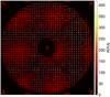 |
Fig. 1 Image from one of the GALACSI LGS-WFS cameras. |
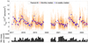 |
Fig. 2 Na vertical column density versus time measured at Paranal (top): all available measurements (orange dots), monthly median (red diamonds) and 15-day median (blue squares); number of measurements for each monthly median (bottom). |
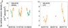 |
Fig. 3 Comparison of Na vertical column density. Left: measured by GALACSI (orange dots) and GRAAL (green dots). Right: measured by GALACSI (orange dots) and LPC (red dots) on chosen nights. |
2.2 CNa retrievals from SCIAMACHY measurements
Vertical Na concentration profiles in the mesopause region were retrieved from daytime limb observations of sunlight resonantly scattered in the Na D-lines, using the SCIAMACHY instrument on ESA’s environmental research satellite Envisat (Burrows et al. 1995; Bovensmann et al. 1999). The nominal SCIAMACHY daytime limb scans did not cover the entire mesopause region, so the retrievals used here are based on a special MLT (Mesosphere – Lower Thermosphere) limb observation mode. Measurements in this mode were carried out between mid 2008 and the end of the Envisat mission in April 2012, twice monthly for a full day each time. These limb measurements covered the tangent height range between 75 and 150 km, providing a complete vertical coverage of the Na D-line emission. It is important to mention that Envisat orbited the Earth in a polar, sun-synchronous orbit with a descending node at 10:00 am local solar time (LST). The LST of the SCIAMACHY daytime limb observations at the latitude of Paranal observatory is about 9:45 LST. The Na profile retrieval methodology has been extensively described in Langowski et al. (2016). Those authors also demonstrated that the SCIAMACHY Na retrieval results are in good agreement with various other observational and modelling datasets, with relative differences typically below 20%. Langowski et al. (2017) conducted a comparison of SCIAMACHY MLT Na profile retrievals with observations by OSIRIS (Llewellyn et al. 2004) on the Earth observation satellite Odin (Murtagh et al. 2002) and an Na climatology based on Global Ozone Monitoring by Occultation of Stars (GOMOS) measurements (Fussen et al. 2010), along with simulations from the WACCM. This study demonstrated good overall agreement among the Na vertical column densities from all observational datasets and the global sodium model simulations.
Figure 4 shows the complete SCIAMACHY dataset, encompassing all available latitudes with measurements averaged over every five degrees of latitude. Within each five-degree latitude range, measurements for all longitudes were used for zonal averaging. This approach is valid since, unlike latitudes that were displaying a significant dependence, no discernible relation to longitude was observed. The measurements are plotted against time, showing all data, together with monthly medians and those over contiguous 15-day windows. The red dashed lines represent the range of ±5 degrees centred around the latitude of 24.6°S, the focus of this CNa study. Figure 5 illustrates all measurements retrieved for this latitude range over time, together with the monthly median and the 15-day median results. The lower plot shows the number of individual measurements obtained for each month. The SCIAMACHY dataset provided consistent and regular coverage across all months of the years of this operational mode. The monthly medians have an average of 17 measurement points (maximum of 25 and minimum of 7).
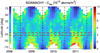 |
Fig. 4 Na vertical column density over time as measured by SCIAMACHY for all latitudes. |
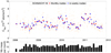 |
Fig. 5 Na vertical column density measured by SCIAMACHY (top): all available measurements (orange dots), monthly median (red diamonds) and 15-day medians (blue squares); number of measurements for each monthly median for the latitude range of 24.6°S±5° (bottom). |
2.3 CNa retrievals from OSIRIS measurements
OSIRIS (McLinden et al. 2012), mounted on the Odin satellite, measured Na (and other terrestrial atmospheric species) profiles in the mesosphere and lower thermosphere with an altitude resolution of 1 km. This was achieved through limb-scattered sunlight. The field of view was 0.02° (vertical) × 0.75° (horizontal), corresponding to 1 km × 40 km at the Earth’s limb. OSIRIS was launched in February 2001 into a sun-synchronous, 6 pm and 6 am local time orbit at an altitude of 620 km. Typically, OSIRIS observations in mid- to high-latitudes were not available in the Northern Hemisphere and in the Southern Hemisphere during their respective winters. Absolute mesospheric Na density profiles were derived from OSIRIS measurements using the method presented in Gumbel et al. (2007).
Figure 6 displays the complete OSIRIS dataset, following the same latitude and time presentation as the SCIAMACHY data. Figure 7 illustrates the complete set of measurements at the latitude of Paranal ± 5 degrees, together with the monthly median and the 15-day median results. The lower plot depicts the number of individual measurements acquired for each month. Significant variations in the number of measurements are observed across different periods of the year. This disparity was caused by Odin’s near-terminator orbit, resulting in notably more daytime observations in the summer hemisphere compared to the winter hemisphere. For the period 2004–2005, no measurements were obtained for certain months. Improved coverage and statistics were available for the years 2008 and 2009. The monthly medians have an average of 190 measurements (maximum of 867 and minimum of 2). In the high Na season (April to September), averages of 35 measurements per month were obtained for 2004–2006, and 131 were obtained for 2007–2009. For the low Na season, averages of 190 measurements per month were obtained for 2004–2006, and 330 were obtained for 2007–2009.
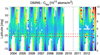 |
Fig. 6 Na vertical column density over time as measured by OSIRIS for all latitudes. |
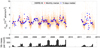 |
Fig. 7 Na vertical column density measured by OSIRIS (top): all available measurements (orange dots), monthly median (red diamonds) and 15-day median (blue squares); number of measurements for each monthly median for the latitude range of 24.6°S±5° (bottom). |
2.4 WACCM4 simulations
In this work, we chose the WACCM-Na results from Dawkins et al. (2016). This represented the longest Na model simulation (1955–2005) from a free-running version of WACCM4 within the first version of Community Earth System Model (CESM1) framework (Hurrell et al. 2013). Na chemistry and the meteoric injection function are based on Marsh et al. (2013). The model accurately simulates the observed Na layer when compared with available LIDAR and satellite measurements (e.g. Marsh et al. 2013; Dunker et al. 2015; Langowski et al. 2017; Feng et al. 2017).
Figure 8 shows the zonally averaged CNa simulated by version 4 of WACCM, with all latitudes presented. The simulations provided a latitude resolution of 1.9 degrees and a longitude resolution of 2.5 degrees. Here, all longitudes have been averaged for each simulated latitude. The simulations were conducted with a temporal resolution of one month.
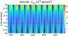 |
Fig. 8 Na vertical column simulated by WACCM4 over time and for all latitudes. |
3 Data analysis and fitting
In our data analysis, our primary objective was to produce a model that fits the available data for the Paranal latitude. Additionally, we aimed to explore whether this model could be used to predict the sodium levels available for LGS applications. To achieve this, we investigated the various contributors to the observed variations, with a specific focus on mid- to long-term effects.
Our three distinct datasets – Paranal, SCIAMACHY, and OSIRIS – and the data simulated by WACCM4 over time at the latitude of 24.6°S are depicted in Fig. 9. To focus on longer timescale variations, we computed the monthly median and the median over 15-day median to the Paranal, SCIAMACHY, and OSIRIS data. Unlike the average, the median is robust against outliers, providing a more reliable estimate of trends. Notably, during periods of overlap between OSIRIS and SCIAMACHY (late 2008 to early 2010, and late 2011 to mid 2012), we observed strong agreement. However, the WACCM4 data, while temporally aligned with SCIAMACHY and OSIRIS, exhibited significant differences in the variations of CNa compared to these two instruments. This result is somewhat surprising, since the WACCM-Na model has been satisfactorily validated against LIDAR measurements at 40°N (Marsh et al. 2013) and higher northern latitudes (Dunker et al. 2015; Langowski et al. 2017; Feng et al. 2017). Thus, while the WACCM-Na model should be a useful tool for predicting the absolute seasonal variations of CNa at many locations, it does not perform as well at the sub-tropical southern latitude of Cerro Paranal. This should be investigated in the future.
WACCM4 simulates reasonable Na abundances when compared with OSIRIS, SCIAMACHY and Paranal observations (Fig. 9), but it is noticeable that this model has produced a larger semi-annual variation over 24.6°S, which requires further investigation. Therefore, we relied solely on measurements from Paranal, SCIAMACHY, and OSIRIS for our objective at modelling the evolution of CNa at 24. 6° S.
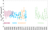 |
Fig. 9 CNa datasets available at latitude of 24.6°S: WACCM4 (red line), OSIRIS (blue dots), SCIAMACHY (orange dots), and Paranal (green dots). The monthly medians are shown here for Paranal, SCIAMACHY, and OSIRIS. |
3.1 Seasonal variations
Astronomical instruments utilising LGSs at Paranal operate every night throughout the year. Understanding the potential variations of CNa over the course of a year is therefore crucial. Our analysis, as depicted in Figs. 2 and 3, revealed significant nocturnal fluctuations. Notably, the median CNa exhibited well established annual and semi-annual periodicities, as documented in previous studies (Simonich et al. 1979; Plane et al. 1999; Hu et al. 2003; Gardner et al. 2005; Clemesha & Batista 2006; Vishnu Prasanth et al. 2009; Fussen et al. 2010; Langowski et al. 2017; Andrioli et al. 2020). To mitigate the impact of night-to-night variations, we computed monthly medians and 15-day period medians to emphasise underlying trends.
Figures 4 and 6 showcase SCIAMACHY and OSIRIS data across a wide range of latitudes, illustrating variations over the year and from one year to the next. As noted in the cited literature, high latitudes are mainly dominated by an annual variation, while semi-annual patterns become more pronounced at mid and low latitudes. Furthermore, these plots highlight significant CNa variations between consecutive years, particularly evident at mid to high latitudes.
The statistical analysis of Paranal data, as depicted in Fig. 10, encompasses several key metrics: the monthly median and the 10th and 90th percentiles. As anticipated based on SCIAMACHY and OSIRIS measurements, we observe both annual and semi-annual variations across years with complete monthly coverage. CNa exhibits a strong annual cycle, peaking between May and July and reaching a minimum in January-February. Notably, CNa rises sharply from April, declines rapidly from July, and flattens out during the September-October period. Subsequent decreases occur in November-December, reaching a minimum in mid-summer. The 10th and 90th percentiles provide insights into the variability encountered each month. Interestingly, the amplitude of monthly variations correlates with the corresponding monthly median. These percentiles do not reveal any distinct annual or semi-annual patterns. It seems that the ratio of the 10th percentile to the median slightly decreases during January and February, as observed in 2019 and 2022 (December and January for the 2017–2018 transition). This suggests that when CNa reaches its lowest median value during the year, the very lowest values are proportionally even lower compared to other periods. Consequently, the lowest CNa encountered during these periods can be exceptionally low. The medians of the measured ratios are as follows: 0.59 ± 0.08 for the 10th percentile and 1.57 ± 0.16 for the 90th percentile. Figure 11 illustrates the distributions of measured CNa for each month, with red dots representing the monthly medians.
Figure 12 illustrates the relative variations of the CNa for each month. These relative variations were computed using two distinct references. The first one, represented by the thick blue (positive variation) and red (negative variation) bars, compares monthly median values to the global mean across the entire available dataset (spanning from 2017 to 2023). This presentation emphasises long-term trends and reveals noticeable differences between years (as explored in Sect. 3.2). The second comparison, displayed by the thin violet (positive variation) and orange (negative variation) bars, represents the relative variations computed using the mean of the corresponding year only. This approach is limited to years with complete monthly coverage. It specifically focuses on variations within a specific year. The detailed results for each year and the comparisons to these two different references are summarised in Table 1. Notably, when using the corresponding year mean as a reference, we observe seasonal variations from the minimum to the maximum for a chosen year ranging from 1.7 (70% increase in 2021) to 2.1 (109% increase in 2023).
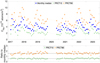 |
Fig. 10 Statistical overview of Na vertical column density over time measured at Paranal. Top: monthly median (blue squares), 10th percentile (green diamonds), and 90th percentile (orange diamonds). Bottom: ratios of the 10th and 90th percentiles in comparison to their respective monthly medians. |
3.2 Fitting
As depicted in Fig. 12, the CNa measured at Paranal exhibits variations between the years that cannot be adequately modelled by considering only annual and semi-annual fluctuations. This global-level variation from year to year is also observed in the OSIRIS and SCIAMACHY data. Hence, at least one longer term effect would be required to derive a model that accounts for these variations. Some studies using LIDAR (Clemesha et al. 1997, She et al. 2023) and meteor radar techniques (Clemesha & Batista 2006) have concluded that there is an influence of the 11-year solar cycle on CNa (and the centroid height). The most comprehensive dataset (to our knowledge), obtained with LIDAR observations at the latitude of 41°N spanning 28 years from 1990 to 2017 (She et al. 2023), shows a solar cycle response of 16.9 ± 2.8% per 100 solar flux units (SFU). We therefore also examined our datasets for potential evidence of a similar influence. The main challenge lies in the fact that the solar cycle has an average length of 11 years, while none of our three instruments’ datasets are long enough to cover at least one cycle. Therefore, the SCIAMACHY and OSIRIS data serve as valuable additions to complement the Paranal dataset for the latitude of 24.6°S.
Our initial attempt at modelling the possible effect of solar activity cycles on CNa was conducted using the Paranal data. As mentioned earlier, during 2017 the GALACSI and GRAAL systems were in a commissioning and testing phase, resulting in less regular and possibly less reliable measurements. For the fitting, we used only the data from January 2018 onward, obtained under stable configurations. The results are presented in Fig. 13, in which we show the complete dataset, the monthly medians, the 15-day period medians, and the fitting to the data (including or excluding solar activity). The fitting was performed using the monthly medians, as this method effectively filtered the short-term variations in CNa for mid-and long-term modelling. Solar activity data, obtained from the LASP Interactive Solar Irradiance Datacenter (LISIRD, https://lasp.colorado.edu/lisird/data), are also presented through the solar radio flux at 10.7 cm. We chose to test the fitting method on this dataset as it comprises a significant number of measurements and provides good coverage of the nights for all the available years. The downside of this dataset is, of course, that it covers only about half a solar cycle.
The following model was used, which includes the annual, semi-annual, and solar cycle:
![Mathematical equation: $\[\begin{aligned}C_{N a}= & \alpha+A_1 \sin \left(2 \pi \frac{t}{365}\right)+A_2 \cos \left(2 \pi \frac{t}{365}\right) \\& +A_3 \sin \left(2 \pi \frac{t}{365 / 2}\right)+A_4 \cos \left(2 \pi \frac{t}{365 / 2}\right)+\delta F_{10.7 a}\end{aligned}\]$](/articles/aa/full_html/2024/11/aa50656-24/aa50656-24-eq1.png) (1)
(1)
with: α the multi-year mean, Ai the fitting coefficients for the annual and semi-annual variations, δ the solar flux fitting, and F10.7a the 81-day moving median of the solar radio flux at F10.7 cm (in SFU). For fitting without solar activity, the last term was of course omitted. A multiple linear regression was used to fit Eq. (1) to the data. When analysing effects linked to the atmosphere, one expects the measurements to be correlated in time to a certain degree, depending on the atmospheric parameter being analysed and the frequency of the measurements compared to the temporal evolution of this parameter. This correlation reduces the number of independent measurements, and this effect was taken into account in the estimation of the uncertainties in the fitting using the methods described in Tiao et al. (1990) and Chiodo et al. (2012). The fitting was performed on both the full Paranal dataset and the monthly medians. The coefficients resulting from the fits are presented in Table 2. The histograms of the data and of the resulting models are depicted in Fig. 14. The goodness of fit, R2, is low when all the data are used; this is due to the high short-term variations on a scale of hours to nights. Using the monthly median to perform the fit increases the goodness of fit, as the high-amplitude short-term variations are filtered out. All the different fits we performed in our study led to very similar results. The correlation between consecutive data points highlights the importance of considering it in the analysis of the uncertainty for the model. The results of the fits including the solar cycle differ significantly when using all the data compared to the monthly median, thus preventing us from drawing any conclusions on this effect. A null-hypothesis test at the 5% level performed to compare the datasets to the different models reported in Table 2 resulted positively for the mean values, but the null hypothesis was rejected in all cases when comparing the standard deviations. The histograms from the models performed on the monthly medians, shown in Fig. 14, do not match the ones from the monthly median exactly; as they clearly miss the highest values of CNa. This mismatch in the standard deviations can be explained by the fact that the highest variations of the CNa measured at Paranal occur on a short timescale; these are not included in our model.
Examining Fig. 13, although the summer minima of each year are well matched, the measured winter maxima are not reached by the models, especially in 2018. Despite the solar activity being at a minimum during that year, the measured Na densities were higher than in years when the Sun was more active. These variations must therefore stem from other effects beyond the scope of this study. The annual and semi-annual variations are well modelled in both fits, with coefficients that match well. However, some shifts in the measured seasonal variations compared to the models are noticeable. While they are well-phased in time for the years 2019 and 2023, the winter increase and maxima are reached earlier than predicted by the model in 2018 and later in 2022. These discrepancies are attributed to natural atmospheric variability.
After testing and validating the fitting method for the Paranal data, we incorporated the SCIAMACHY and OSIRIS data into our analysis, allowing us to span more than one solar cycle. In this context, it is crucial to ensure that data from different instruments, using distinct measuring methods, exhibit sensible agreement. As shown earlier, this is confirmed between SCIAMACHY and OSIRIS during overlapping periods. Unfortunately, there is no overlap of the Paranal data with either of the two satellite datasets, so we assume that the individual measurements of CNa are well calibrated and accurately reported. During our analysis, it became evident that we needed to be cautious regarding the sizes of the three datasets to avoid biasing the results. We thus used the monthly medians for all three datasets. Furthermore, as observed in Fig. 7, OSIRIS data during the winter months are mostly missing for the initial years or have considerably lower data availability compared to the summer months. During the data analysis and fitting tests, this was found to lead to inconsistent results compared to the other datasets. Neither the annual cycle nor the semi-annual cycle are well represented when using the complete OSIRIS dataset for the Paranal latitude. Therefore, we additionally limited the OSIRIS data to October to March, where the amount of available data is high.
With the data selected as described above, we performed the fit using Eq. (1). The results are presented in Table 3 and plotted in Fig. 15. The fit to the Paranal-only monthly medians, not including the solar cycle effect, is also shown for comparison. The two fits give close results, with the most significant differences being in the phase of the annual variations and the amplitude of the semi-annual one. Figure 15 shows generally good agreement between the different fits and the data, with variations mostly dominated by the seasonal ones.
Relative variations of Na vertical column density for each year compared to the global dataset mean (left values) and to their yearly mean (right values).
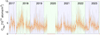 |
Fig. 11 Na vertical column-density monthly distributions for Paranal: histogram of the measurements obtained for each month (orange), and median values of each month (red dots). |
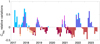 |
Fig. 12 Na vertical column density monthly relative variations. |
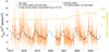 |
Fig. 13 Na vertical column density at Paranal. All data (orange dots), monthly median (red diamonds), and two fitting scenarios: considering the solar cycle (black dashed line) and not considering the solar cycle (blue solid line). Solar activity is indicated by the 81-day moving median of the solar flux at 10.7 cm measured in solar flux units (SFU). |
CNa fitting coefficients for Paranal dataset, with or without the solar cycle influence.
CNa fitting coefficients for the monthly medians of all data sets together, with or without the solar cycle influence.
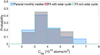 |
Fig. 14 Comparison of histogram distribution of CNa between the Paranal data and the model with and without the Sun activity. |
4 Discussion
Figure 2 illustrates the high variability in measured CNa at Paranal, showcasing fluctuations across diverse timescales. The LGS, whose return flux is utilised for LGS-WFS measurements, is generated in the Na layer aligned with the telescope’s observation direction. The laser beam creating the LGS has a diameter of approximately 75 cm at the altitude of the Na layer (representing the 1/e2 width for a Gaussian beam, for a 1 arcsec spot at the mesospheric altitude of 90 km). This relatively small beam diameter makes it sensitive to local effects on small spatial scales. Sporadic Na layers in the mesosphere have been documented by Clemesha (1995), Batista et al. (1989), Friedman et al. (2000), O’Sullivan et al. (2000), and Pfrommer et al. (2009). The rapid amplitude variations of CNa in the Paranal data on a scale of less than an hour can be adequately explained by this effect, along with disturbances induced by short-period atmospheric gravity waves (Fritts et al. 2018). This underlines the importance of obtaining measurements, ideally with a frequency of minutes during significant portions of a night, and covering as many nights as possible in a continuous manner. The Paranal systems achieve this effectively, and they are frequently employed for scientific observations.
For mid- and long-term variations in CNa, a monthly median proved to be an effective low-pass filter for shorter timescale variations. Although a 15-day median was also considered during the analysis, it was found to be less efficient at filtering night-to-night variations occurring within a month. We opted for the median over the mean for its robustness against potential outliers. While alternatives were considered such as computing the median for each night when measurements were available, or using all available data, they led to difficulty in comparing the model to the data because of the significant short timescale variations not addressed in this modelling attempt. Consequently, the monthly median was selected to analyse all datasets in this study.
To optimise the design of LGSs-based AO systems and maximise their performance, understanding the statistical variations in the return flux from the Na layer, both in time and amplitude, is crucial. Through extensive use of the GALACSI and GRAAL systems at Paranal, we amassed a significant statistical sample comprising approximately 126 500 individual measurements. These were obtained over many nights spanning a period of six years, with an interruption in 2020 during the COVID-19 pandemic. Clear annual and semi-annual variations are evident in the dataset. The winter peak spans about four months, with a notable rise starting around April and a decline from July onwards. A plateau is consistently seen in the spring time before a second decrease leading into the summer minimum from December to February. Measurements at Paranal indicate winter enhancements ranging between 1.7 and 2.1, closely matching seasonal variations observed by LIDAR at a similar latitude in São José dos Campos (Brazil, 23°S), where a factor of two is reported (Simonich et al. 1979). This seasonal amplitude varies with latitude; mid-latitudes such as Illinois (40°N) and Colorado (41°N) have reported factors of three (Plane et al. 1999), while polar regions exhibit ratios up to ten (Gardner et al. 1988, Gardner et al. 2005). Although the distribution of CNa for a given month shows considerable variability (see Fig. 11), we also demonstrate that the ratios between the 10th and 90th percentiles remain relatively constant compared to the median value (Fig. 10).
Our data analysis did not provide conclusive evidence of the solar cycle’s influence on the Na layer. This effect has been explored in previous studies, yielding varying conclusions. Simonich et al. (1979), using LIDAR data obtained at 23°S, suggested a variation in Na abundance due to the solar cycle. However, with only five years of data, they faced the same challenge as our study, emphasising the need for more extensive and longer spanning data for confirmation. In a study focusing on the vertical distribution of the Na layer using LIDAR data from the same location, Clemesha et al. (1997) concluded that the solar cycle caused a small variation in the centroid height of the layer. Subsequently, in a study covering almost three solar cycles from 1972 to 2001, the same group (Clemesha et al. 2004) found no discernible effect of the solar cycle on the centroid height of the Na layer. Another study (Clemesha & Batista 2006), using meteor radar data from 2000 to 2005 to analyse changes in meteor ablation height at a latitude of 23°S, suggested a possible detection of a solar cycle effect. This series of studies, conducted at the same location and partially with the same data, vividly illustrates the challenge of finding evidence (or lack thereof) of the solar cycle’s influence, given its small amplitude compared to seasonal variations. Indeed, Dawkins et al. (2016) reported an insignificant solar-cycle dependence (<1% per 100 SFU at all latitudes) on the Na layer from 50 years of WACCM4 simulations between 1955 and 2005. However, in a recent study (She et al. 2023) using 28 years of LIDAR data obtained at latitudes 41°N and 42°N at Colorado and Utah State universities (CSU, USU), a clear correlation between the Na layer’s vertical column density and the solar flux was established. The authors reported an influence of the solar cycle of 16.9 ± 2.8% per 100 SFU. During our investigation, productive discussions with Prof. Chiao-Yao facilitated a comparison of our method with his data at 41°N. Using a model similar to She et al. (2023), differing only in the linear trend, we applied our fitting method to the CSU and USU datasets and independently obtained a very similar value for the influence of the solar cycle at 41°N.
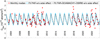 |
Fig. 15 Monthly Na vertical column density versus time measured at latitude of 24.6°S, gathering the Paranal, SCIAMACHY, and OSIRIS data (red diamonds); model derived from fitting only the Paranal monthly medians (blue dashed line) and from fitting the monthly medians of the three datasets together (black dotted line). |
5 Conclusions
We analysed variations in the vertical column density, CNa, at the latitude of 24.6°S corresponding to the Paranal Observatory, using the flux measured by the LGS-WFSs of the AOF, in conjunction with measurements from the SCIAMACHY and OSIRIS space instruments. The LGS-WFSs systems were not originally designed for measuring Na density in the atmosphere, and we validated the extraction of CNa from these instruments by comparing them with measurements from an independent system also installed at the Paranal Observatory. The CNa computed with this new method also align well with levels measured by LIDAR at a similar latitude but different times, as reported in Simonich et al. (1979). There is good agreement of CNa with measurements from the SCIAMACHY (Langowski et al. 2016) and OSIRIS space-based instruments, which allowed us to extend the time coverage from 2004 to 2023 and search for long-term trends. Larger variations in CNa are observed in the Paranal dataset compared to those found in the SCIAMACHY and OSIRIS data. One possible reason for this is that the Paranal data are exclusively nighttime observations, taken over most of each night, whereas the satellite data is restricted to daytime observations at set local times (where changes in atmospheric tides might have a greater effect).
With 126 500 independent measurements obtained over 1115 nights spanning six years at Paranal, we have compiled an essential statistical database for Na vertical column density, crucial for designing AO systems. This database provides insights into variations across various timescales. Short-term variations on the scale of minutes allow us to evaluate their impact on realtime control for atmospheric turbulence correction. Variations over the course of a night offer crucial insights into managing and optimising AO systems to ensure consistent performance during astronomical observations. We also demonstrated that the LGSs can be relatively dim in the southern summer following seasonal variations, reaching very low values during the summer minimum. Conversely, the LGSs can become very bright during winter owing to sporadic Na events in the upper and lower mesosphere. Through careful analysis of Na vertical column density at the latitude of the Paranal Observatory, we developed a model for the mid- and long-term evolution of CNa over time, as indicated by the fit coefficients in Table 2. The design of AO systems using LGSs must consider these effects, and the substantial Paranal database is invaluable for achieving this.
Acknowledgements
The SCIAMACHY Na profile retrievals were in part supported by the European Space Agency (ESA) through the MesosphEO project, by the University of Greifswald and the University of Bremen. SCIAMACHY was jointly funded by Germany (DLR), the Netherlands (NSO) and Belgium. We are indebted to ESA for providing the SCIAMACHY Level 1 data used. We are grateful to Pr. Chiao-Yao She for the fruitful discussions and insights for the analysis and understanding of our data. D.R.M. is supported in part by Natural Environment Research Council Grant NE/V018442/1, MesoS2D: Mesospheric sub-seasonal to decadal predictability. W.F. and J.M.C. Plane were supported by the European Research Council (project number 291332 – CODITA) and the UK Natural Environment Research Council (NERC grant NE/G019487/1).
References
- Andrioli, V., Xu, J., Batista, P., et al. 2020, J. Geophys. Res. Space Phys., 125, e2019JA027493 [CrossRef] [Google Scholar]
- Batista, P. P., Clemesha, B. R., Batista, I. S., & Simonich, D. M. 1989, J. Geophys. Res., 94, 15349 [NASA ADS] [CrossRef] [Google Scholar]
- Bernard, R. 1938, Nature, 142, 164 [CrossRef] [Google Scholar]
- Bovensmann, H., Burrows, J. P., Buchwitz, M., et al. 1999, J. Atmos. Sci., 56, 127 [NASA ADS] [CrossRef] [Google Scholar]
- Burrows, J. P., Hölzle, E., Goede, A. P. H., Visser, H., & Fricke, W. 1995, Acta Astronaut., 35, 445 [NASA ADS] [CrossRef] [Google Scholar]
- Carrillo-Sánchez, J. D., Gómez-Martín, J. C., Bones, D. L., et al. 2020, Icarus, 335, 445 [Google Scholar]
- Castro-Almazán, J., Alonso, A., Bonaccini Calia, D., et al. 2017, in AO4ELT5 [Google Scholar]
- Chiodo, G., Calvo, N., Marsh, D. R., & Garcia-Herrera, R. 2012, J. Geophys. Res., 117 [Google Scholar]
- Clemesha, B. R. 1995, J. Atmos. Terres. Phys., 57, 725 [NASA ADS] [CrossRef] [Google Scholar]
- Clemesha, B., & Batista, P. 2006, J. Atmos. Sol.-Terres. Phys., 68, 1934 [NASA ADS] [CrossRef] [Google Scholar]
- Clemesha, B., Batista, P., & Simonich, D. 1997, J. Atmos. Sol.-Terres. Phys., 59, 1673 [NASA ADS] [CrossRef] [Google Scholar]
- Clemesha, B. R., Simonich, D. M., & Batista, I. S. 2004, J. Geophys. Res., 109, D11306 [Google Scholar]
- Dawkins, E. C. M., Plane, J. M. C., Chipperfield, M. P., et al. 2016, J. Geophys. Res. Space Phys., 121, 7153 [NASA ADS] [CrossRef] [Google Scholar]
- Dunker, T., Hoppe, U.-P., Feng, W., Plane, J. M., & Marsh, D. R. 2015, J. Atmos. Sol.-Terres. Phys., 127, 111 [NASA ADS] [CrossRef] [Google Scholar]
- Feng, W., Kaifler, B., Marsh, D. R., et al. 2017, J. Atmos. Sol.-Terres. Phys., 162, 162 [NASA ADS] [CrossRef] [Google Scholar]
- Friedman, J. S., González, S. A., Tepley, C. A., et al. 2000, Geophys. Res. Lett., 27, 449 [NASA ADS] [CrossRef] [Google Scholar]
- Fritts, D. C., Vosper, S. B., Williams, B. P., et al. 2018, J. Geophys. Res. Atmos., 123, 9992 [NASA ADS] [CrossRef] [Google Scholar]
- Fussen, D., Vanhellemont, F., Tétard, C., et al. 2010, Atmos. Chem. Phys., 10, 9225 [NASA ADS] [CrossRef] [Google Scholar]
- Gardner, C. S., Senft, D. C., & Kwon, K. H. 1988, Nature, 332, 142 [CrossRef] [Google Scholar]
- Gardner, C. S., Plane, J. M. C., Pan, W., et al. 2005, J. Geophys. Res. Atmos., 110, 718 [Google Scholar]
- Gumbel, J., Fan, Z. Y., Waldemarsson, T., et al. 2007, Geophys. Res. Lett., 34, 15 [CrossRef] [Google Scholar]
- Haguenauer, P. 2022, SPIE, 12185, 1218512 [NASA ADS] [Google Scholar]
- Holzlöhner, R., Rochester, S. M., Bonaccini Calia, D., et al. 2010a, A&A, 510, A20 [NASA ADS] [CrossRef] [EDP Sciences] [Google Scholar]
- Holzlöhner, R., Rochester, S., Pfrommer, T., et al. 2010b, SPIE, 7736, 77365D [Google Scholar]
- Hu, X., Gardner, C. S., & Liu, A. Z. 2003, Chinese J. Geophys., 46, 432 [CrossRef] [Google Scholar]
- Hurrell, J. W., Holland, M. M., Gent, P. R., et al. 2013, Bull. Am. Meteorol. Soc., 94, 1339 [CrossRef] [Google Scholar]
- Langowski, M. P., von Savigny, C., Burrows, J. P., et al. 2016, Atmos. Meas. Tech., 9, 295 [NASA ADS] [CrossRef] [Google Scholar]
- Langowski, M. P., von Savigny, C., Burrows, J. P., et al. 2017, Atmos. Meas. Tech., 10, 2989 [NASA ADS] [CrossRef] [Google Scholar]
- Llewellyn, E. J., Lloyd, N. D., Degenstein, D. A., et al. 2004, Can. J. Phys., 82, 411 [NASA ADS] [CrossRef] [Google Scholar]
- Madec, P.-Y., Arsenault, R., Kuntschner, H., et al. 2018, SPIE, 10703, 1 [Google Scholar]
- Marsh, D. R., Janches, D., Feng, W., & Plane, J. M. C. 2013, J. Geophys. Res. Atmos., 118, 11442 [NASA ADS] [CrossRef] [Google Scholar]
- McLinden, C. A., Bourassa, A. E., Brohede, S., et al. 2012, Bull. Am. Meteorol. Soc., 93, 1845 [CrossRef] [Google Scholar]
- Murtagh, D., Frisk, U., Merino, F., et al. 2002, Can. J. Phys., 80, 309 [NASA ADS] [CrossRef] [Google Scholar]
- Neichel, B., D’Orgeville, C., Callingham, J., et al. 2013, MNRAS, 429, 3522 [NASA ADS] [CrossRef] [Google Scholar]
- O’Sullivan, C., Redfern, R. M., Ageorges, N., et al. 2000, Exp. Astron., 10, 147 [CrossRef] [Google Scholar]
- Pfrommer, T., & Hickson, P. 2014, A&A, 565, A102 [EDP Sciences] [Google Scholar]
- Pfrommer, T., Hickson, P., & She, C.-Y. 2009, Geophys. Res. Lett., 36, 15 [CrossRef] [Google Scholar]
- Plane, J. M. C., Gardner, C. S., Yu, J., et al. 1999, J. Geophys. Res., 104, 3773 [NASA ADS] [CrossRef] [Google Scholar]
- Plane, J. M. C., Feng, W., & Dawkins, E. C. M. 2015, Chem. Rev., 115, 4497 [CrossRef] [Google Scholar]
- She, C.-Y., Krueger, D. A., Yan, Z.-A., Yuan, T., & Smith, A. K. 2023, J. Geophys. Res. Space Phys., 128, e2023JA031652 [NASA ADS] [CrossRef] [Google Scholar]
- Simonich, D. M., Clemesha, B. R., & Kirchhoff, V. W. J. H. 1979, J. Geophys. Res. Space Phys., 84, 1543 [NASA ADS] [CrossRef] [Google Scholar]
- Slipher, V. M. 1929, PASP, 41, 262 [NASA ADS] [Google Scholar]
- Tiao, G., Reinsel, G., Xu, D., et al. 1990, J. Geophys. Res., 95, 20507 [NASA ADS] [CrossRef] [Google Scholar]
- Vishnu Prasanth, P., Sivakumar, V., Sridharan, S., et al. 2009, Annal. Geophys., 27, 3811 [NASA ADS] [CrossRef] [Google Scholar]
All Tables
Relative variations of Na vertical column density for each year compared to the global dataset mean (left values) and to their yearly mean (right values).
CNa fitting coefficients for Paranal dataset, with or without the solar cycle influence.
CNa fitting coefficients for the monthly medians of all data sets together, with or without the solar cycle influence.
All Figures
|
Fig. 1 Image from one of the GALACSI LGS-WFS cameras. |
| In the text | |
|
Fig. 2 Na vertical column density versus time measured at Paranal (top): all available measurements (orange dots), monthly median (red diamonds) and 15-day median (blue squares); number of measurements for each monthly median (bottom). |
| In the text | |
|
Fig. 3 Comparison of Na vertical column density. Left: measured by GALACSI (orange dots) and GRAAL (green dots). Right: measured by GALACSI (orange dots) and LPC (red dots) on chosen nights. |
| In the text | |
|
Fig. 4 Na vertical column density over time as measured by SCIAMACHY for all latitudes. |
| In the text | |
|
Fig. 5 Na vertical column density measured by SCIAMACHY (top): all available measurements (orange dots), monthly median (red diamonds) and 15-day medians (blue squares); number of measurements for each monthly median for the latitude range of 24.6°S±5° (bottom). |
| In the text | |
|
Fig. 6 Na vertical column density over time as measured by OSIRIS for all latitudes. |
| In the text | |
|
Fig. 7 Na vertical column density measured by OSIRIS (top): all available measurements (orange dots), monthly median (red diamonds) and 15-day median (blue squares); number of measurements for each monthly median for the latitude range of 24.6°S±5° (bottom). |
| In the text | |
|
Fig. 8 Na vertical column simulated by WACCM4 over time and for all latitudes. |
| In the text | |
|
Fig. 9 CNa datasets available at latitude of 24.6°S: WACCM4 (red line), OSIRIS (blue dots), SCIAMACHY (orange dots), and Paranal (green dots). The monthly medians are shown here for Paranal, SCIAMACHY, and OSIRIS. |
| In the text | |
|
Fig. 10 Statistical overview of Na vertical column density over time measured at Paranal. Top: monthly median (blue squares), 10th percentile (green diamonds), and 90th percentile (orange diamonds). Bottom: ratios of the 10th and 90th percentiles in comparison to their respective monthly medians. |
| In the text | |
|
Fig. 11 Na vertical column-density monthly distributions for Paranal: histogram of the measurements obtained for each month (orange), and median values of each month (red dots). |
| In the text | |
|
Fig. 12 Na vertical column density monthly relative variations. |
| In the text | |
|
Fig. 13 Na vertical column density at Paranal. All data (orange dots), monthly median (red diamonds), and two fitting scenarios: considering the solar cycle (black dashed line) and not considering the solar cycle (blue solid line). Solar activity is indicated by the 81-day moving median of the solar flux at 10.7 cm measured in solar flux units (SFU). |
| In the text | |
|
Fig. 14 Comparison of histogram distribution of CNa between the Paranal data and the model with and without the Sun activity. |
| In the text | |
|
Fig. 15 Monthly Na vertical column density versus time measured at latitude of 24.6°S, gathering the Paranal, SCIAMACHY, and OSIRIS data (red diamonds); model derived from fitting only the Paranal monthly medians (blue dashed line) and from fitting the monthly medians of the three datasets together (black dotted line). |
| In the text | |
Current usage metrics show cumulative count of Article Views (full-text article views including HTML views, PDF and ePub downloads, according to the available data) and Abstracts Views on Vision4Press platform.
Data correspond to usage on the plateform after 2015. The current usage metrics is available 48-96 hours after online publication and is updated daily on week days.
Initial download of the metrics may take a while.