| Issue |
A&A
Volume 691, November 2024
|
|
|---|---|---|
| Article Number | A279 | |
| Number of page(s) | 7 | |
| Section | Extragalactic astronomy | |
| DOI | https://doi.org/10.1051/0004-6361/202450616 | |
| Published online | 19 November 2024 | |
Detection of the Fe K lines from the binary AGN in 4C+37.11
1
Indian Institute of Astrophysics, 2nd Block Koramangala, Bangalore, 560034 Karnataka, India
2
Institute of Theoretical Astrophysics, University of Oslo, P.O box 1029 Blindern, 0315 OSLO, Norway
3
National Radio Astronomy Observatory, Socorro, NM 87801, USA
4
School of Physical Sciences, National Institute of Science Education and Research, Bhubaneswar An OCC of Homi Bhabha National Institute, Jatni -752050, India
5
Department of Physics and Astronomy, University of New Mexico, Albuquerque NM 87131, USA
⋆ Corresponding author; This email address is being protected from spambots. You need JavaScript enabled to view it.
; This email address is being protected from spambots. You need JavaScript enabled to view it.
Received:
6
May
2024
Accepted:
9
September
2024
Abstract
We report the discovery of the Fe K line emission at ∼6.62−0.06+0.06 keV with a width of ∼0.19−0.05+0.05 keV using two epochs of Chandra archival data for the nucleus of the galaxy 4C+37.11, which is known to host a binary supermassive black hole (BSMBH) system where the SMBHs are separated by ∼7 mas or ∼7pc. Our study reports the first detection of the Fe K line from a known binary AGN, which has an F-statistic value of 20.98 and a probability of 2.47 × 10⁻¹². Stacking two spectra reveals another Fe K line component at ∼7.87−0.09+0.19 keV. Different model scenarios indicate that the lines originate from the combined effects of accretion disk emission and circumnuclear collisionally ionized medium. The observed low column density favors a gas-poor merger scenario, where the high temperature of the hot ionized medium may be associated with the shocked gas in the binary merger and not with star formation activity. The estimated total BSMBH mass and disk inclination are ∼1.5 × 10¹⁰ M⊙ and ≳75°, indicating that the BSMBH is probably a high-inclination system. We were not able to tightly constrain the spin parameter using the present data sets. Our results draw attention to the fact that detecting the Fe K line emissions from BSMBHs is important for estimating the individual SMBH masses and the spins of the binary SMBHs, as well as for exploring their emission regions.
Key words: accretion / accretion disks / radiative transfer / Galaxy: nucleus / galaxies: interactions / galaxies: jets
© The Authors 2024
 Open Access article, published by EDP Sciences, under the terms of the Creative Commons Attribution License (https://creativecommons.org/licenses/by/4.0), which permits unrestricted use, distribution, and reproduction in any medium, provided the original work is properly cited.
This article is published in open access under the Subscribe to Open model. This email address is being protected from spambots. You need JavaScript enabled to view it. to support open access publication.
1. Introduction
Binary supermassive black holes (BSMBHs) are rare systems that may form during galaxy mergers (Begelman et al. 1980). When both the SMBHs are accreting mass, they become active galactic nuclei (AGN), and can be referred to as a binary AGN (< 100 pc), or dual AGN (DAGN; > 10 kpc) depending on their separation (Burke-Spolaor et al. 2014; Rubinur et al. 2019). Although there have been several detections of dual AGN, the detection of binary AGN is more challenging as it requires very high-resolution observations over different energy bands (e.g., see a recent review by De Rosa et al. 2019). These systems are important for understanding the final stages of galaxy mergers, especially when the SMBHs are separated by a few parsecs, as then they can become gravitationally bound. When this happens, the binary SMBH system can emit gravitational waves that will contribute to the gravitational wave background (Agazie et al. 2023). Several surveys in multiwavelength bands are focused on searching for DAGN and binary AGN (Abazajian et al. 2009; Wright et al. 2010; Ahn et al. 2012; Lena et al. 2018, and references therein).
So far, less than 200 DAGN systems have been detected (Rubinur et al. 2018; Bhattacharya et al. 2023). Only a few of them (e.g., 4C+37.11, NGC7674) are separated on parsec scales and have been detected with high-resolution Very Long Baseline Array (VLBA) observations (Rodriguez et al. 2006; Kharb et al. 2017). However, a recent study has claimed a nondetection of the radio core in NGC 7674 (Breiding et al. 2022), suggesting the requirement for a further in-depth analysis of the binary AGN system. Instead, most AGN pairs have been identified at kiloparsec (kpc) scale separations (DAGN), where the two nuclei may not be bound by mutual gravitational effects (Owen et al. 1985; Komossa et al. 2003; Bhattacharya et al. 2023). Of the binary AGN detected, 4C+37.11 is the most well-studied example. It is a radio galaxy at redshift z = 0.055, harboring a binary AGN system where the two cores (designated C1 and C2 in Figure 1) are separated by ∼7 pc (Maness et al. 2004; Rodriguez et al. 2006). A prominent jet (C2 in Figure 1) is also observed from one of the nuclei in the VLBA radio image (Bansal et al. 2017).
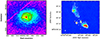 |
Fig. 1. Image of the core of 4C+37.11 in X-rays and radio wavelength. Left: The X-ray image obtained from Chandra observation. The red circle is the region of 12″ considered for spectral analysis. Right: Naturally weighted VLBA map of the zoomed-in central core region at 8 GHz, where the beam size along the jet direction is 1.26 mas (Bansal et al. 2017). The central core components are designated C1 and C2 with negative contours in magenta. The contour levels are 0.6, 1.25, 5, 10, 40, and 60% of the peak flux density 0.0792 Jy/beam. |
Depending on the separation between the AGN, the mass accretion may change, as the gravitational potential of one affects the other. Therefore, it is quite natural to see effects in the spectral properties. Among the several complex features in X-ray AGN spectra, the presence of the Fe Kα line and its shape are very important as they can provide valuable information regarding the accretion disk geometry, spin parameters, and physical processes occurring close to the SMBH. It is believed that the power-law spectrum in the hard X-ray band becomes modified by emission and absorption processes, which arise due to the reprocessing of radiation by cold material in the accretion disk or by more distant material such as that in the torus (Magdziarz & Zdziarski 1995; Chakrabarti & Titarchuk 1995; Nandra et al. 2007; García et al. 2013, and references therein). One of the signatures of such reprocessing is the presence of the Fe Kα line. Therefore, this line carries information about the dynamical state and thermodynamics of the reprocessing material. For example, if the disk moves much closer and reprocesses the radiation, this latter should be reflected in the shape of the Fe Kα, and should therefore be double peaked, for example, due to rotation and asymmetry owing to relativistic effects (see e.g., Fabian et al. 1989; Iwasawa et al. 1996; Brenneman & Reynolds 2006; Mondal et al. 2016, and references therein). A recent study of DAGN using Chandra reported strong neutral lines from both nuclei in the merger remnant NGC 6240 (Nardini 2017).
Though the different types of AGN show different features in their Fe Kα line, the width of the Fe Kα can be a valuable probe of the emission region. Typically, equivalent widths (EWs) of ∼1 keV are associated with absorbed sources, such as distant material or a torus, while EWs of ∼0.1 keV point to unabsorbed sources such as accretion disks or broad line regions. The broad iron lines, and the associated Compton reflection continuum, are generally weak or absent in the radio-loud (RL) counterparts (Eracleous et al. 1996; Reynolds & Begelman 1997; Sambruna et al. 1999; Grandi et al. 1999). This can be due to the washing out of a typical “Seyfert-like” X-ray spectrum by a Doppler-boosted jet component, or the inner disk may be unable to produce reflection features because it is in a very hot state. At the same time, it has been found that a broad component of the Fe Kα line is present in many radio-quiet (RQ; “nonjetted") AGNs (Nandra et al. 1997; Patrick et al. 2012; Mantovani et al. 2016). Also, it is important to note that the broad line profiles help to constrain the spin parameter of the BH (for a recent review see Reynolds 2019).
A systematic analysis of a sample of 149 RQ type-1 AGNs by de La Calle Pérez et al. (2010) using XMM-Newton data found that 36% of the sources show strong evidence of a relativistic Fe Kα line. The average EW of this line is of the order of 100 eV. Therefore, the question of whether or not a broad Fe line is commonly present in RL or RQ AGNs remains open. Earlier studies reported the identification of a broad Fe Kα line in a few individual RL AGNs (Lohfink et al. 2015). However, very few of them have robust spin measurements. Similarly, the narrow Fe Kα lines observed in X-ray spectra are interpreted as fluorescence lines from neutral (cold) matter away from the inner accretion disk. Propositions have been put forward as to the origin of the narrow emission line, which include the molecular torus, the broad line regions, or the very outermost regions of the accretion disk (Jiang et al. 2006).
Hence, independent of the merging process and the formation of DAGN, one can ask whether or not the spectrum of closely separated DAGN or a binary AGN system appear similar to that of an isolated AGN disk spectrum. As in the case of 4C+37.11, it may also be possible that one AGN is contributing to the observed spectrum, while the other is not emitting very actively. In this study, we have tried to answer these questions by analyzing the X-ray spectrum of the binary AGN system 4C+37.11 based on Chandra archival data. In the following section (Sect. 2), we discuss the observation details and data analysis. We discuss our results and findings in Sect. 3, and finally present our conclusions.
2. Observation and data analysis
We use archival Chandra observations (ids: 16120, 12704; hereafter O1 and O2) of 4C+37.11 obtained on November 6, 2013 and April 4, 2011. The exposure times of the observations are ∼95 ks and ∼11 ks, respectively. The Chandra data were reprocessed with CIAO (v.4.14) using the updated calibration files (v.4.9.6). The level 2 event files were recreated by the script of chandra_repro. The source was extracted from the circular region with a radius of 12″ and the background with a radius of 30″. The Chandra image of the source and the corresponding source region (red circle) are shown in the left panel of Figure 1. The right panel of Figure 1 shows the VLBA image of the zoomed-in central core region of 4C+37.11 at 8 GHz. The core components are C1 and C2, where C1 appears to be compact and C2 shows a prominent jet emanating from the central AGN (Bansal et al. 2017). The spectra of source and background, as well as the response files, were produced using the specextract script. We could not find significant pile-up1 (< 7%) for either spectrum. The spectra were binned using the grppha tool to ensure ten counts per spectral bin before exporting to xspec for analysis (Reynolds & Miller 2010). The spectral analysis was carried out for the energy range 0.7−8 keV. We tried a different source region of 6″, which does not change the spectral shape, but lowers the number of data points in the whole spectrum. Different models available in XSPEC (v.12.12.0) are used to fit the data from both observations. The spin parameter (a) is estimated directly from the kerrdisk spectral model (Brenneman & Reynolds 2006) fitting. These model fits give accretion properties, radiation processes, and most importantly the intrinsic parameters of the BH (e.g., spin). All errors are estimated at the 1σ confidence level throughout the paper using err task.
3. Results and discussion
First, we fitted the O1 data using a simple power-law ( pl) model to fit the continuum, which returns a statistically poor fit with χ2= 583 for 293 degrees of freedom (d.o.f.) and a photon index (Γ) of 2.59 ± 0.04. We then performed the same fitting by adding a zgauss component to the fit to detect the Fe K line. This improves the fit with χ2 = 279 for 290 d.o.f. and Γ = 2.75 ± 0.05. The Fe K line fits at energy ∼6.66 ± 0.02 keV with σE ∼ 82.7 ± 26.5 eV. In general, Fe Kα emission is often observed at 6.4 keV. However, other Fe K lines can be found in the 6–7 keV band, such as Fe XXV at 6.63–6.70 keV and Fe XXVI at 6.97 keV (see Ponti et al. 2009; Patrick et al. 2012, and references therein). Therefore, hereafter, we refer to the detected line as the Fe K line. We further ran the ftest task in xspec to check the requirement of the zgauss component, which yields an F-statistic value = 20.98 and a probability of 2.47 × 10⁻¹², which corresponds to a 6.9σ confidence level. We fitted the O2 observation using the same model and detect the presence of the Fe K line at 6.66 ± 0.11 keV; however, due to the lower number of data points, we could not constrain the line width ( eV). There is little difference between model fittings with (χ2 = 81 for 81 d.o.f.) and without (χ2 = 86 for 84 d.o.f.) the zgauss component, which could be due to the shorter exposure time. The F statistic value is 1.67 and the probability is 0.18, which corresponds to the 0.9σ level. As the Fe K line is clearly visible in our spectrum, we adopted the F-test method to determine the detection level of the emission line in O1, following approaches in the literature (see Ponti et al. 2009; Tombesi et al. 2010; Liu et al. 2010; Hu et al. 2019; Liu et al. 2024, and others).
Additionally, the spectrum (especially in O1) also shows a soft excess below 2 keV (see also, Arnaud et al. 1985; Singh et al. 1985). For the soft excess and the presence of optically thin collisionally ionized plasma, the apec model is used, while other additive models are used to take into account the Fe K line. To obtain more insight into the system and the origin of the line, we used two different classes of models. The first class are single-continuum models: M1: ztbabs( apec+ zgauss), M2: tbabs( apec+ laor), M3: tbabs( apec+ kerrdisk), and M4: ztbabs( xillver+ zgauss), and the second class are two-continuum models: M5: ztbabs( apec+ apec) and M6: ztbabs( relxill+ apec). These models cover both the contribution of ionized plasma due to shocked gas and the star formation activity in the host galaxy, distant reflection, and relativistic effects on the origin of the Fe K line. We first discuss the results from our analysis using the first set of models and then the second set. Finally, we draw conclusions based on the results from the second set of models.
3.1. Analysis with single-continuum models
We started the model fitting using a single-component apec model, which we found to be unable to fit the entire line in the O1 observation as χ2 = 357 for 290 d.o.f. Therefore, we fitted the O1 spectrum using the M1 model, yielding a satisfactory fit with χ2= 330 for the 287 d.o.f. This model helps to determine the Fe K line properties (e.g., width and energy) qualitatively. The Fe K line fits at ∼6.62 ± 0.06 keV with the σg ∼ 0.19 ± 0.05 keV for O1, while the O2 spectrum does not require the zgauss component. The EW of the line in O1 spectrum estimated to be ∼0.36 keV using eqwidth task. Based on the σg value of the line in O1, it can be considered as a broad Fe K line. The O2 spectrum is well fit with M1 (without zgauss component), and the model provides kTe =  keV and
  Z⊙. The hydrogen column density NH obtained from the M1 model is
  cm−2 (for O1) and
  cm−2 (for O2) using the ztbabs model (Wilms et al. 2000), which takes into account the X-ray absorption through the interstellar medium (ISM). The model fitted parameters are given in tab:SpecFit. The spectrum fitted with the M1 model for O1 is shown in the left panel of Fig. 2. Additionally, we show the confidence contour between the line energy and line width, and the Δχ2 contour of the line energy. The contours are shown in the middle and right panels of Fig. 2. The red, green, and blue lines in the middle panel correspond to the 1σ, 2σ, and 3σ confidence, respectively. The dashed horizontal lines in the right panel correspond to different significance levels of the uncertainty on the position of the Fe K line. As the Fe K line is broad and can originate from different regions of the SMBH and its vicinity, we first tested emission line models with relativistic effects.
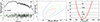 |
Fig. 2. Analysis of O1 spectrum of binary AGN 4C+37.11 using model M1. Left: Best-fitted O1 spectrum in the 0.7−7.5 keV energy range. Points and solid line in the top panel denote the data and model while the model fitted residual is shown in the bottom panel. The line width of the Fe Kα line is ∼0.19 ± 0.05 keV. Middle: Confidence contour between the line energy and line width. The red, green, and blue contours correspond 1σ, 2σ, and 3σ levels. Right: Δχ2 confidence contour of the Fe Kα line energy. The dashed horizontal lines represent different confidence levels of the detection. |
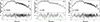 |
Fig. 3. M6 model fitted to the spectra of the binary AGN 4C+37.11 in the 0.7−8 keV energy range. The left panel shows the best fit for observation O1, and the middle panel shows that for O2. The right panel shows the best-fitted stacked spectrum. The lower panels show the corresponding residuals of the fits. |
During M2 model fitting to the O1 observation, we varied both the qcrlaor (Laor 1991) and qcrapec model parameters. During this fitting, we kept the outer radius of the disk Rout fixed to 400 rg ( = GMBH/c2). The best-fit emissivity index (q) and disk inclination (i) obtained from the fit are  and
and  , respectively. The inner edge of the disk (Rin) is pegged at the lower limit, 1.24 rg. The qcrapec model parameters obtained from the fit are consistent with M1 model parameters.
To further obtain an initial qualitative estimate of the BH spin parameter, we fitted the data using model M3, where a similar procedure as in M2 was followed. For the M3 fitting, we varied some of the qcrkerrdisk (Brenneman & Reynolds 2006) model parameters. During this fitting, we fixed the break radius (Rbr) separating the inner (Rin) and outer radii of the disk (Rout) to ∼10 rg, i to 86°, and Rin to 1.24 rg obtained from the M2 fitting, keeping qcrapec model parameters free. The dimensionless spin parameter obtained from the best fit is  and the emissivity index (q2k) =
  . As Rin could not be constrained from the M2 model and the ak parameter in M3 has a large error bar, the spin parameter (ak), which can have a large degeneracy (see Fabian et al. 2014), cannot be tightly constrained. The qcrapec model parameter values obtained from the fit are consistent with those provided by M1 and M2. We note that as the Fe K line is not very significant in the O2 observation due to low statistics, we were not able to use M2 and M3 to constrain the model parameters. All model-fitted results are provided in Table 1.
Best-fit spectral model parameters.
In the next step of the analysis, we studied the possibility that the Fe line originates from a distant reflector, mainly from the toroidal region, using the qcrxillver model (García et al. 2013). As the qcrapec model can also partly contribute to the emission line, we used qcrxillver as a standalone case without considering the qcrapec component. During M4 model fitting, we left the qcrxillver model parameters to vary. An independent nonrelativistic qcrxillver model can fit the Fe K line. However, the overall spectrum fits with χ2/d.o.f. = 367/285 ∼ 1.3, which is a relatively poor fit compared to other models. The best fit to the O1 observation returned Γ= , an Fe abundance (AFe) of =
  Z⊙, an ionization parameter of (log ξ) =
  , an electron temperature of the corona (kTe) pegged at 400 keV, and a disk inclination of (i) =
  . As we used qcrxillver as a single-component model without the qcrapec model, achieving the best fit required a qcrzgauss component at ∼0.8 keV to fit the excess emission around that energy. The O2 data fitting using the M4 model returned
  ,
,  Z⊙,
Z⊙,  ,
,  keV, and
  . In these two epochs, all model parameters except NH, Γ, and kTe remained approximately constant within the error bars over a timescale of two and a half years.
3.2. Analysis with two-continuum models
The models M1–M4 provide some initial qualitative information on the properties of the Fe K line. None of these models describe the realistic emission from an accretion disk. Therefore, the question remains as to whether the Fe K lines originate from the accretion disk or the material unaffected by strong dynamical effects. To address this question, we further used the second set of two-continuum qcrapec and relativistic reflection qcrrelxill models (Dauser et al. 2014; Garcia et al. 2014). Given that a single-component qcrapec model alone cannot fit the data well, we added another qcrapec component (M5), which can fit the O1 spectrum well with χ2 = 329 for 287 d.o.f. The temperature and abundances of the ionized mediums in the qcrapec model components in M5 are  keV and
  keV, and
  and
and  respectively. The M5 model can successfully take into account the Fe K line as well. The NH obtained from the M5 model is
  ×1022 cm−2. Therefore, the origin of the Fe K line could be due to multicomponent, optically thin, collisionally ionized plasma. For the O2 spectral fitting, we did not require the additional qcrapec component.
Subsequently, we used the relativistic reflection-based qcrrelxill model (M6), which takes into account accretion disk emissions more realistically and comprehensively. This model uses an empirical broken power-law emissivity and a cutoffpl spectral shape for the central source. The qcrrelxill model has 14 parameters, of which several can be fixed to reasonable values in order to avoid degeneracy in the best-fit parameters, as has been done by several authors in the literature (see, Inaba et al. 2022; Mondal et al. 2024, and references therein). From the remaining parameters, we chose a nonrotating BH, as keeping it free does not allow us to constrain its value, since the spin parameter (a) always reaches to its upper hard limit of 0.998. This also affects in constraing the other parameters. Additionally, we were not able to constrain the a parameter from the M3 model either. Such tasks prompted us to set a to zero in M6. The following qcrrelxill model parameters cannot be constrained given the statistical quality and unavailability of the broadband data: the inner edge of the disk (Rin), Ecut, the reflection fraction (Rref), and the emissivity indexes (index1 and index2), and so we fixed them to astrophysically motivated values and continued the modeling in the next step of the analysis.
The inner and outer edges of the disk, Rin and Rout, are set to RISCO and 1000 rg, respectively. The parameter Rbr determines a break radius that separates two regimes with different emissivity profiles and is set to 10 rg. We fixed the emissivity indexes at 2.4 and the reflection fraction Rref at -0.25 to obtain only the reflected component. The above choices were made following the previous DAGN analysis by Inaba et al. (2022, and references therein). The kTe was fixed to values obtained from the qcrxillver model (M4) fitting. The remaining parameters, i, Γ, and log ξ, were allowed to vary. We note that fitting the spectrum using the qcrrelxill model with these educated guesses did not produce the observed Fe K line, and therefore we added an qcrapec component. The combined model reads in XSPEC as M6. The model fit returns an acceptable fit with χ2/d.o.f. = 324/285. The best-fitting model for the O1 spectrum returns  ,
,  ,
,  , and
, and  Z⊙. The O2 spectral fitting gives
  ,
,  , and
, and  with AFe pegged at the lower limit of 0.5 Z⊙. Such a significantly low value of AFe compared to O1 could be due to the limited number of data points in the spectrum. In order to investigate this matter further, we redid the fit, this time freezing the AFe value to that found for the O1 spectrum, which returned a comparable fit in terms of χ2 and model parameter values.
The ξ fitted with the M6 model is high for both O1 and O2, which is expected as the Fe K line originates from a region containing two accreting SMBHs; one of the AGN has radio jets, and such regions may contain highly ionized plasma. Our estimated line energy follows the estimation of ξ as discussed in the literature (Kallman et al. 2004; Ponti et al. 2009; Patrick et al. 2012). The estimated absorbed total fluxes using M6 in the energy band 0.7–8.0 keV are 1.12 and 1.28 ×10⁻¹² ergs cm−2 s−1 for the epochs O1 and O2, respectively. All parameters from the M6 model fit are given in tab:SpecFit and the best-fitted M6 spectra are shown in the left and middle panels of fig:SpecMod2. As both M5 and M6 models can fit the Fe K line satisfactorily, to quantify their contribution, we calculated the relative fraction of the line intensity in the 6.0–7.0 keV band due to qcrapec and qcrrelxill in M6. If Iapec and Irelxill are the line intensities from each model, then the relative fractions due to the qcrapec and qcrrelxill models are Iapec/(Iapec+Irelxill) ∼60% and Irelxill/(Iapec+Irelxill) ∼40%, respectively. Therefore, collisionally ionized plasma contributes more to the Fe K line.
The M1–M6 model fits to the O1 spectrum showed another line feature above 7.5 keV (see left panels of fig:SpecZgauss and fig:SpecMod2). However, the data statistic at that line energy is poor. Therefore, we stacked both spectra, which shows a clear line feature at higher energy. We fitted this line component by adding another qcrzgauss component to M1 to find the line properties, which gives  keV with
  keV, keeping the qcrapec model parameters unchanged. Further, we fitted the stacked spectrum using the M6 model by adding another qcrzgauss component for the second Fe K line, which gives
  keV with
  keV, k
 keV, and
  in the qcrapec model. The other qcrrelxill model parameters are
  ,
,  ,
,  , and
, and  , and kTe was fixed at 400 keV. The model fits the data very well, with χ2 = 317 for 291 d.o.f. The best-fitting model spectrum is shown in the right panel of fig:SpecMod2. The line feature at ∼7.8 − 7.9 keV could be the emission line due to Fe Kβ or Ni Kα, or a mixture of both coming from distant material. The difference in peak line energies also indicates that those may not be coming from the individual nuclei, as the relative velocity required to obtain such a large energy difference (ΔE > 1.2 keV ∼0.19c) exceeds the escape velocity of the BSMBH system (∼0.01c for the system mass of ∼1010 M⊙ and a separation of 7 pc, orbiting in circular orbit). This indicates that these lines originate from distant ionized material. However, as this is a binary system, the scenario might be more complex, and therefore follow-up studies are required to better constrain the Fe K lines and their origin.
The NH value obtained from the M6 model shows a significant change over 2.5 years between epochs, but this change is not very large, at ≤1.5 × 1022 cm−2. It has been shown that the star formation rates (SFRs) and AGN fractions are expected to increase as a function of decreasing pair separation of mergers (e.g., Ellison et al. 2008), and so we generally expect to find dual or binary AGNs in gas-rich environments, and therefore in regions with an elevated SFR. However, recent galaxy-merger simulations showed that both SFR and circumnuclear obscuration (in terms of NH) become weaker in gas-poor mergers than in gas-rich ones (Blecha et al. 2018), which also depends on the gas-to-mass ratio of the host galaxy (Inaba et al. 2022). The 4C+37.11 is an elliptical galaxy. It is observed that in elliptical galaxies either the gas contain is little or no star formation activities (Romani et al. 2014). Hence, there is probably little gas associated with star formation in our system as well. Our results favor a gas-poor merger scenario. On the other hand, the change in hot ionized gas temperatures in M1 between O1 and O2 and in qcrapec model components (M5) in O1 could be due to shocked gas associated with the binary environment, and possibly not due to star formation activity.
Given the best-fitting M6 model parameters and luminosities (LX ∼8.2 and 9.1 × 1042 erg s−1) for both observations, the location of the ionized medium can be derived from the definition of ξ (Tarter et al. 1969) as R ∼ LX/NHξ ∼ 0.7 − 1.1 × 1018 cm. The estimation of the R is based on assumptions that the medium has a constant density and the thickness of the medium does not exceed its distance from the central SMBH (e.g., Crenshaw & Kraemer 2012; Mestici et al. 2024). Ionized mediumthat can produce the emission lines can be composed of outflowing gas (King & Pounds 2003) arising from within 1 pc scale region of the central SMBH that can block the central radiation. If we assume that the broadening of the Fe K line is due to the velocity of the distant outflowing gas, we can obtain the velocity from the EW measurement using  , which yields v ≈0.05c. Here, c, FWHM, and E0 are the speed of light, the full-width at half maximum of the line (from M1 fit), and the rest-frame energy of the Fe K line (∼6.6 keV). If one equates this velocity with the escape velocity of the outflowing gas within the gravitational potential of the central SMBH at a distance R, then the total mass of the BSMBH is found to be ∼1.2 − 1.7 × 10¹⁰ M⊙, with an average of ∼1.5 × 10¹⁰ M⊙. Our estimation agrees with an estimation based on radio observations (Bansal et al. 2017).
4. Conclusion
In this paper, we studied two Chandra observations of a binary AGN 4C+37.11 observed during 2013 (obs. O1) and 2011 (obs. O2). We report the detection of the Fe K lines at  keV (with 6.9σ confidence using F-test) of width
  keV (1σ confidence) and another line feature at
  keV of width
  keV from the stacking of two spectra in the binary AGN system 4C+37.11, where the SMBHs are separated by ∼7 pc. Here, we briefly discuss the origin of the Fe K line from the model-fitted parameters.
The consideration of a simple fluorescent line (model M1) fits the lines well and provides the properties of the Fe K lines. However, the M1 model cannot infer their origin, as the system contains two black holes, both of which have accretion disks, one of them contains a radio jet, and the circumnuclear region is associated with ionized gas. Therefore, we used two sets of models; the first is a single-continuum model (M1–M4) and the second is a two-continuum model (M5–M6). The former sets of models can give us preliminary information on the nature of the lines and qualitative information on the emissivity properties of the accretion disk. It is believed that the effect of spin or the origin of the Fe K line from the very inner edge of the disk can leave their footprint as a broadening or skewing of the line profile. As the Fe K lines in 4C+37.11 are broad, if this were due to relativistic effects, then model M3 should be able to constrain the spin parameter; however, we find this not to be the case. This may be eVidence that the lines did not originate from the accretion disk and further motivates a study using models that consider the distant reflection. The M4 model can fit the Fe K line independently, but the overall fit statistic is poor (reduced χ2 ∼ 1.3). The failure of extensive tests with single-continuum models to provide promising results prompted us to further use the two-continuum models (M5 and M6), especially the qcrrelxill model, which takes into account emission from an accretion disk realistically.
A two-continuum collisionally ionized plasma model (qcrapec, M5) can fit the observed Fe K line profile, which infers a possible origin of the line from a circumnuclear environment. The above model fits can constrain the temperature and abundance of the scattering medium, where the abundances of the material vary between subsolar and supersolar regimes. Later, we used the M6 model, which can fit the line profile and the continuum with acceptable fit statistics; this further favors a scenario where the line profiles originate from the combined effects of the accretion disk and the circumnuclear environment. The high values of both Fe abundance and ionization parameters suggest that the Fe K lines possibly originate from highly ionized medium. This is also reflected in the line energy, which is shifted by 0.2 keV compared to the neutral Fe Kα line. As the M6 model takes into account emission from both the accretion disk and collisionally ionized plasma, and provides additional information about the system, we favor this model over M5 based on the present study.
From the data fitted by two sets of models, we propose the following conclusions:
-
Single-continuum models along with line emission (M1–M4) cannot explain the origin of Fe K lines, but provide the initial line properties qualitatively.
-
Both two-continuum models (M5 and M6) can represent the line properties satisfactorily, suggesting the line originates from the circumnuclear ionized medium. This suggests an origin in combined effects rather than in the accretion disk in isolation.
-
The best-fitting qcrrelxill model suggests the inclination of the disk is ≳75° and that the medium from where the line originates is highly ionized (log ξ ≳ 2.7) with sub- to supersolar Fe abundance. We estimate the total mass of the BSMBH using the M6 model parameters and luminosity to be ∼1.5 × 10¹⁰ M⊙.
-
The low nuclear obscuration (in terms of NH in M6) in the elliptical galaxy 4C+37.11 supports the gas-poor merger scenario more than elevated star formation activity. Also, the significant change in the temperature of the hot ionized medium could be associated with the shocked gas in the binary merger and not with the SFR.
-
We were not able to constrain the inner edge of the disk (Rin) or the spin parameter (a) from the present analysis.
-
We note that M5 and M6 are alternative scenarios, and therefore one can only derive constraints on a and Rin of the accretion flow if the M6 model is the correct representation of the data, and no statement on the same quantities can be drawn if M5 is the correct description.
Follow-up broadband X-ray observations are needed to understand this system in detail. Furthermore, onboard and future microcalorimeters such as X-Ray Imaging and Spectroscopy Mission (XRISM; XRISM Science Team 2020) and Advanced Telescope for High Energy Astrophysics (Athena; Barret et al. 2016) will help in studying the origin of such lines due to their high spectroscopic resolution, and will possibly be able to further confirm the detection presented here. For the radio observations, we have adequate resolution, but additional observations are needed to better constrain the orbital parameters of the binary black hole system. In the optical band, the Hβ line detection can provide further clues about the emission region of the Fe K lines (Nandra 2006), if such lines can be detected in the future.
Acknowledgments
We thank the referee for making thoughtful comments and suggestions that help improve the quality of the paper. SM thanks V. Liu for helping with some analysis. SM acknowledges the Ramanujan Fellowship (RJF/2020/000113) by DST-SERB, Govt. of India for this research. M.D. acknowledges the support of the Science and Engineering Research Board (SERB) CRG grant CRG/2022/004531 for this research. AN acknowledges the Summer Research Fellowship program of IAS, INSA, NASI for providing financial support. The National Radio Astronomy Observatory is a facility of the National Science Foundation operated under cooperative agreement by Associated Universities, Inc. This research has made use of data obtained from the Chandra Data Archive and the Chandra Source Catalog, and software provided by the Chandra X-ray Center (CXC) in the application packages CIAO and made use of the NuSTAR Data Analysis Software (NUSTARDAS) jointly developed by the ASI Science Data Center (ASDC), Italy and the California Institute of Technology (Caltech), USA. This research has also made use of data obtained through the High Energy Astrophysics Science Archive Research Center Online Service, provided by NASA/Goddard Space Flight Center.
References
- Abazajian, K. N., Adelman-McCarthy, J. K., Agüeros, M. A., et al. 2009, ApJS, 182, 543 [Google Scholar]
- Agazie, G., Anumarlapudi, A., Archibald, A. M., et al. 2023, ApJ, 951, L8 [NASA ADS] [CrossRef] [Google Scholar]
- Ahn, C. P., Alexandroff, R., Allende Prieto, C., et al. 2012, ApJS, 203, 21 [Google Scholar]
- Arnaud, K. A., Branduardi-Raymont, G., Culhane, J. L., et al. 1985, MNRAS, 217, 105 [NASA ADS] [CrossRef] [Google Scholar]
- Bansal, K., Taylor, G. B., Peck, A. B., Zavala, R. T., & Romani, R. W. 2017, ApJ, 843, 14 [NASA ADS] [CrossRef] [Google Scholar]
- Barret, D., Lam Trong, T., den Herder, J.-W., & Piro, L. 2016, Proc. SPIE, 9905, 99052F [NASA ADS] [CrossRef] [Google Scholar]
- Begelman, M. C., Blandford, R. D., & Rees, M. J. 1980, Nature, 287, 307 [Google Scholar]
- Bhattacharya, A., Nehal, C. P., Das, M., et al. 2023, MNRAS, 524, 4482 [CrossRef] [Google Scholar]
- Blecha, L., Snyder, G. F., Satyapal, S., & Ellison, S. L. 2018, MNRAS, 478, 3056 [Google Scholar]
- Breiding, P., Burke-Spolaor, S., An, T., et al. 2022, ApJ, 933, 143 [NASA ADS] [CrossRef] [Google Scholar]
- Brenneman, L. W., & Reynolds, C. S. 2006, ApJ, 652, 1028 [NASA ADS] [CrossRef] [Google Scholar]
- Burke-Spolaor, S., Brazier, A., Chatterjee, S., et al. 2014, MNRAS, 524, 4482 [Google Scholar]
- Chakrabarti, S., & Titarchuk, L. G. 1995, ApJ, 455, 623 [NASA ADS] [CrossRef] [Google Scholar]
- Crenshaw, D. M., & Kraemer, S. B. 2012, ApJ, 753, 75 [NASA ADS] [CrossRef] [Google Scholar]
- Dauser, T., Garcia, J., Parker, M. L., Fabian, A. C., & Wilms, J. 2014, MNRAS, 444, L100 [Google Scholar]
- de La Calle Pérez, I., Longinotti, A. L., Guainazzi, M., et al. 2010, A&A, 524, A50 [CrossRef] [EDP Sciences] [Google Scholar]
- De Rosa, A., Vignali, C., Bogdanović, T., et al. 2019, New Astron. Rev., 86, 101525 [Google Scholar]
- Ellison, S. L., Patton, D. R., Simard, L., & McConnachie, A. W. 2008, AJ, 135, 1877 [NASA ADS] [CrossRef] [Google Scholar]
- Eracleous, M., Halpern, J. P., & Livio, M. 1996, ApJ, 459, 89 [NASA ADS] [CrossRef] [Google Scholar]
- Fabian, A. C., Rees, M. J., Stella, L., & White, N. E. 1989, MNRAS, 238, 729 [Google Scholar]
- Fabian, A. C., Parker, M. L., Wilkins, D. R., et al. 2014, MNRAS, 439, 2307 [NASA ADS] [CrossRef] [Google Scholar]
- García, J., Dauser, T., Reynolds, C. S., et al. 2013, ApJ, 768, 146 [Google Scholar]
- Garcia, J., Dauser, T., Lohfink, A., et al. 2014, ApJ, 782, 76 [NASA ADS] [CrossRef] [Google Scholar]
- Grandi, P., Guainazzi, M., Haardt, F., et al. 1999, A&A, 343, 33 [NASA ADS] [Google Scholar]
- Hu, J., Liu, Z., Jin, C., & Yuan, W. 2019, MNRAS, 488, 4378 [NASA ADS] [CrossRef] [Google Scholar]
- Inaba, K., Ueda, Y., Yamada, S., et al. 2022, ApJ, 939, 88 [NASA ADS] [CrossRef] [Google Scholar]
- Iwasawa, K., Fabian, A. C., Reynolds, C. S., et al. 1996, MNRAS, 282, 1038 [NASA ADS] [CrossRef] [Google Scholar]
- Jiang, P., Wang, J. X., & Wang, T. G. 2006, ApJ, 644, 725 [NASA ADS] [CrossRef] [Google Scholar]
- Kallman, T. R., Palmeri, P., Bautista, M. A., Mendoza, C., & Krolik, J. H. 2004, ApJS, 155, 675 [Google Scholar]
- Kharb, P., Lal, D. V., & Merritt, D. 2017, Nature Astronomy, 1, 727 [NASA ADS] [CrossRef] [Google Scholar]
- King, A. R., & Pounds, K. A. 2003, MNRAS, 345, 657 [Google Scholar]
- Komossa, S., Burwitz, V., Hasinger, G., et al. 2003, ApJ, 582, L15 [NASA ADS] [CrossRef] [Google Scholar]
- Laor, A. 1991, ApJ, 376, 90 [Google Scholar]
- Lena, D., Panizo-Espinar, G., Jonker, P. G., Torres, M. A. P., & Heida, M. 2018, MNRAS, 478, 1326 [NASA ADS] [CrossRef] [Google Scholar]
- Liu, Y., Elvis, M., McHardy, I. M., et al. 2010, ApJ, 710, 1228 [NASA ADS] [CrossRef] [Google Scholar]
- Liu, V., Zoghbi, A., & Miller, J. M. 2024, ApJ, 963, 38 [NASA ADS] [CrossRef] [Google Scholar]
- Lohfink, A. M., Ogle, P., Tombesi, F., et al. 2015, ApJ, 814, 24 [NASA ADS] [CrossRef] [Google Scholar]
- Magdziarz, P., & Zdziarski, A. A. 1995, MNRAS, 273, 837 [Google Scholar]
- Maness, H. L., Taylor, G. B., Zavala, R. T., Peck, A. B., & Pollack, L. K. 2004, ApJ, 602, 123 [NASA ADS] [CrossRef] [Google Scholar]
- Mantovani, G., Nandra, K., & Ponti, G. 2016, MNRAS, 458, 4198 [NASA ADS] [CrossRef] [Google Scholar]
- Mestici, S., Tombesi, F., Gaspari, M., Piconcelli, E., & Panessa, F. 2024, MNRAS, 532, 3036 [NASA ADS] [CrossRef] [Google Scholar]
- Mondal, S., Chakrabarti, S. K., & Debnath, D. 2016, Ap&SS, 361, 309 [NASA ADS] [CrossRef] [Google Scholar]
- Mondal, S., Chatterjee, R., Agrawal, V. K., & Nandi, A. 2024, Pub. Astron. Soc. Aust., submitted [arXiv:2403.14169] [Google Scholar]
- Nandra, K. 2006, MNRAS, 368, L62 [NASA ADS] [CrossRef] [Google Scholar]
- Nandra, K., George, I. M., Mushotzky, R. F., Turner, T. J., & Yaqoob, T. 1997, ApJ, 488, L91 [NASA ADS] [CrossRef] [Google Scholar]
- Nandra, K., O’Neill, P. M., George, I. M., & Reeves, J. N. 2007, MNRAS, 382, 194 [NASA ADS] [CrossRef] [Google Scholar]
- Nardini, E. 2017, MNRAS, 471, 3483 [NASA ADS] [CrossRef] [Google Scholar]
- Owen, F. N., O’Dea, C. P., Inoue, M., & Eilek, J. A. 1985, ApJ, 294, L85 [NASA ADS] [CrossRef] [Google Scholar]
- Patrick, A. R., Reeves, J. N., Porquet, D., et al. 2012, MNRAS, 426, 2522 [NASA ADS] [CrossRef] [Google Scholar]
- Ponti, G., Cappi, M., Vignali, C., et al. 2009, MNRAS, 394, 1487 [NASA ADS] [CrossRef] [Google Scholar]
- Reynolds, C. S. 2019, Nature Astronomy, 3, 41 [NASA ADS] [CrossRef] [Google Scholar]
- Reynolds, C. S., & Begelman, M. C. 1997, ApJ, 487, L135 [NASA ADS] [CrossRef] [Google Scholar]
- Reynolds, M. T., & Miller, J. M. 2010, ApJ, 723, 1799 [NASA ADS] [CrossRef] [Google Scholar]
- Rodriguez, C., Taylor, G. B., Zavala, R. T., et al. 2006, ApJ, 646, 49 [Google Scholar]
- Romani, R. W., Forman, W. R., Jones, C., et al. 2014, ApJ, 780, 149 [Google Scholar]
- Rubinur, K., Das, M., & Kharb, P. 2018, JApA, 39, 8 [Google Scholar]
- Rubinur, K., Das, M., & Kharb, P. 2019, MNRAS, 484, 4933 [Google Scholar]
- Sambruna, R. M., Eracleous, M., & Mushotzky, R. F. 1999, ApJ, 526, 60 [NASA ADS] [CrossRef] [Google Scholar]
- Singh, K. P., Garmire, G. P., & Nousek, J. 1985, ApJ, 297, 633 [NASA ADS] [CrossRef] [Google Scholar]
- Tarter, C. B., Tucker, W. H., & Salpeter, E. E. 1969, ApJ, 156, 943 [Google Scholar]
- Tombesi, F., Cappi, M., Reeves, J. N., et al. 2010, A&A, 521, A57 [NASA ADS] [CrossRef] [EDP Sciences] [Google Scholar]
- Wilms, J., Allen, A., & McCray, R. 2000, ApJ, 542, 914 [Google Scholar]
- Wright, E. L., Eisenhardt, P. R. M., Mainzer, A. K., et al. 2010, AJ, 140, 1868 [Google Scholar]
- XRISM Science Team 2020, arXiv e-prints [arXiv:2003.04962] [Google Scholar]
All Tables
All Figures
|
Fig. 1. Image of the core of 4C+37.11 in X-rays and radio wavelength. Left: The X-ray image obtained from Chandra observation. The red circle is the region of 12″ considered for spectral analysis. Right: Naturally weighted VLBA map of the zoomed-in central core region at 8 GHz, where the beam size along the jet direction is 1.26 mas (Bansal et al. 2017). The central core components are designated C1 and C2 with negative contours in magenta. The contour levels are 0.6, 1.25, 5, 10, 40, and 60% of the peak flux density 0.0792 Jy/beam. |
| In the text | |
|
Fig. 2. Analysis of O1 spectrum of binary AGN 4C+37.11 using model M1. Left: Best-fitted O1 spectrum in the 0.7−7.5 keV energy range. Points and solid line in the top panel denote the data and model while the model fitted residual is shown in the bottom panel. The line width of the Fe Kα line is ∼0.19 ± 0.05 keV. Middle: Confidence contour between the line energy and line width. The red, green, and blue contours correspond 1σ, 2σ, and 3σ levels. Right: Δχ2 confidence contour of the Fe Kα line energy. The dashed horizontal lines represent different confidence levels of the detection. |
| In the text | |
|
Fig. 3. M6 model fitted to the spectra of the binary AGN 4C+37.11 in the 0.7−8 keV energy range. The left panel shows the best fit for observation O1, and the middle panel shows that for O2. The right panel shows the best-fitted stacked spectrum. The lower panels show the corresponding residuals of the fits. |
| In the text | |
Current usage metrics show cumulative count of Article Views (full-text article views including HTML views, PDF and ePub downloads, according to the available data) and Abstracts Views on Vision4Press platform.
Data correspond to usage on the plateform after 2015. The current usage metrics is available 48-96 hours after online publication and is updated daily on week days.
Initial download of the metrics may take a while.