| Issue |
A&A
Volume 691, November 2024
|
|
|---|---|---|
| Article Number | A26 | |
| Number of page(s) | 13 | |
| Section | Astrophysical processes | |
| DOI | https://doi.org/10.1051/0004-6361/202450414 | |
| Published online | 29 October 2024 | |
Exploring the intermittency of magnetohydrodynamic turbulence by synchrotron polarization radiation
1
Department of Physics, Xiangtan University, Xiangtan, Hunan 411105, PR China
2
Key Laboratory of Stars and Interstellar Medium, Xiangtan University, Xiangtan 411105, PR China
3
Department of Astronomy and Space Science, Chungnam National University, Daejeon, Republic of Korea
⋆ Corresponding authors; jfzhang@xtu.edu.cn, lufang0810@xtu.edu.cn
Received:
17
April
2024
Accepted:
9
September
2024
Context. Magnetohydrodynamic (MHD) turbulence plays a critical role in many key astrophysical processes, such as star formation, acceleration of cosmic rays, and heat conduction. However, its properties are still poorly understood.
Aims. In this work, we explore how to extract the intermittency of compressible MHD turbulence from synthetic and real observations.
Methods. We used three statistical methods, namely the probability distribution function, kurtosis, and scaling exponent of the multi-order structure function, to reveal the intermittency of MHD turbulence.
Results. Our numerical results demonstrate that: (1) the synchrotron polarization intensity statistics can be used to probe the intermittency of magnetic turbulence, by which we can distinguish different turbulence regimes; (2) the intermittency of MHD turbulence is dominated by the slow mode in the sub-Alfvénic turbulence regime; and (3) the Galactic interstellar medium (ISM) in the low latitude region corresponds to the sub-Alfvénic and supersonic turbulence regime.
Conclusions.We have successfully measured the intermittency of the Galactic ISM from synthetic and realistic observations.
Key words: magnetohydrodynamics (MHD) / polarization / radiation mechanisms: non-thermal / ISM: magnetic fields / ISM: structure
© The Authors 2024
 Open Access article, published by EDP Sciences, under the terms of the Creative Commons Attribution License (https://creativecommons.org/licenses/by/4.0), which permits unrestricted use, distribution, and reproduction in any medium, provided the original work is properly cited.
This article is published in open access under the Subscribe to Open model. Subscribe to A&A to support open access publication.
1. Introduction
Intermittency is one of the properties of magnetohydrodynamic (MHD) turbulence and has been studied in the solar wind (Veltri 1999; Carbone et al. 2004; Chen et al. 2014; Wang et al. 2015), interplanetary medium (Bruno et al. 2007; Zelenyi et al. 2015), magnetosphere (Xu et al. 2023), and interstellar medium (ISM) (McKee & Ostriker 1977; Rickett 2011; Falgarone et al. 2011; Fraternale et al. 2019). This intermittency, associated with a small-scale coherent structure, can influence interstellar gas heating (Osman et al. 2011, 2012a,b; Wu et al. 2013; Chen et al. 2020; Phillips et al. 2023), energy dissipation (Zhdankin et al. 2016; Wan et al. 2012; Huang et al. 2022), and increased temperature anisotropy (Servidio et al. 2012; Osman et al. 2012b) in plasma turbulence. Moreover, this coherent structure plays an important role in particle acceleration (Décamp & Malara 2006; Lemoine 2021; Vega et al. 2023) and scattering (Butsky et al. 2024). Therefore, studying this intermittency is important in understanding and interpreting several astrophysical processes.
When neglecting the intermittency effect, Kolmogorov (1941) predicted that the power-law index ζp of the structure function of velocity fluctuations is proportional to its order p in the inertial range, that is, ζp = p/3. The intermittency is ubiquitous in turbulence environments such as the solar wind (e.g., Osman et al. 2014) and diffusion ISM (e.g., Falgarone et al. 2011). When factoring in the intermittency, the relation between the order and the power-law index is expected to be a nonlinear behavior. Indeed, later studies found that the scaling exponent ζp gradually deviates from the linear relation of ζp = p/3 as the order p increases (Anselmet et al. 1984; Meneveau & Sreenivasan 1987; Białas & Seixas 1990; Vincent & Meneguzzi 1991). To understand this phenomenon, two modified models have been proposed to describe incompressible hydrodynamic (She & Leveque 1994) and MHD turbulence (Müller & Biskamp 2000), respectively (see Section 2.1, as well as Biskamp 2003; Beresnyak & Lazarian 2019 for more details).
The intermittency of MHD turbulence has been extensively investigated in numerical simulations (Falgarone & Passot 2008; Biskamp 2003; Esquivel & Lazarian 2010). For the incompressible homogeneous MHD turbulence, Yoshimatsu et al. (2011) concluded that the magnetic field is more intermittent than the velocity, consistent with other works (Cho et al. 2003; Haugen et al. 2004; Mallet & Schekochihin 2017). For the compressible MHD turbulence, Kowal et al. (2007) claimed that the density intermittency strongly depends on Alfvénic and sonic Mach numbers, with the velocity intermittency being different from the density one.
The later simulations confirmed that the intermittency of MHD turbulence is closely related to its compressibility, scale-dependent anisotropy, and magnetization. For instance, it was found that the intermittency of three plasma modes (Alfvén, slow, and fast) increases with the sonic Mach number in the weak magnetic field (Kowal & Lazarian 2010). The viscosity-damped MHD turbulence shows scale-dependent intermittency, that is, greater intermittency at much smaller scales (Cho et al. 2003). With respect to the latter, Davis et al. (2024) concludes that with increasing magnetization, the velocity fluctuations display an inverse trend of the co-dimension of structures compared to the magnetic field. Yang et al. (2018) also advances that the effect of the MHD turbulence amplitude on the distribution of the magnetic field is preferred to that of the angle to the local magnetic field. It has also been found that the intermittency is associated with the turbulence driving mechanism (Federrath et al. 2008, 2009; Beattie et al. 2022). Based on centroid velocity statistics, Federrath et al. (2010) found that the intermittency for compressive forcing is stronger than that for solenoidal forcing.
We note that there have been various studies on measuring MHD turbulence intermittency in solar physics and astrophysics. In the former, with the solar wind data from the STEREO spacecraft, Osman et al. (2014) measured the intermittency of magnetic and Els sser field fluctuations in the solar wind and found that the intermittency in the direction perpendicular to the local magnetic field is stronger than that in the parallel direction. Considering density fluctuations, Chen et al. (2014) also found strong intermittency ranging from ion to electron scales. In astrophysics, the turbulence in molecular clouds exhibits small-scale and inertial-range intermittency (Hily-Blant et al. 2008). In addition, Falgarone et al. (2011) found the non-Gaussian statistic results and the existence of coherent structures in the diffuse ISM.
As mentioned above, intermittency has been measured using spectroscopic data of the ISM and in situ data of the solar wind. We seek to understand whether we can use synchrotron polarization observations to extract the intermittency of MHD turbulence. One purpose of our numerical studies is to explore the intermittency of magnetic fields and densities via synthetic observations. Another purpose is to study the intermittency of the Galactic ISM using realistic observations. For this work, we first synthesized synchrotron polarization observations using numerical simulation data to study the intermittency of the magnetic field and density, and then adopted realistic observations from the Canadian Galactic Plane Survey (CGPS). From an observational perspective, this work sought to advance the understanding of the intermittency of compressible MHD turbulence.
This paper is organized as follows. In Section 2, we describe the theoretical models of the intermittency, synchrotron radiative processes, and methods to characterize intermittency. Section 3 introduces the numerical setup and the decomposed method of compressible MHD turbulence. Section 4 presents the numerical results, followed by the studies of intermittency from the observational data in Section 5. The discussion and summary are provided in Sections 6 and 7.
2. Theories and methods
2.1. Theoretical models related to intermittency
In the framework of incompressible hydrodynamic turbulence, Kolmogorov (1941) assumed that the turbulence is self-similar within the inertial range, in which the relationship between the velocity fluctuations δul and the scale l exhibits a simple scaling behavior as follows:
When the scaling exponent ζp deviates from this relation, it implies the appearance of the intermittency phenomenon, which reflects the inhomogeneous distribution of fluctuations (see Chap. 7 in Biskamp 2003). Later, taking the scaling of velocity ul ∼ l1/g and energy cascade rate t−1 ∼ l−x into account, She & Leveque (1994) analytically proposed a classical nonlinear scaling expressed as
where C denotes the co-dimension of the dissipative structures related to the dimension of a dissipative structure D via the relation C = 3 − D.
In the case of hydrodynamic turbulence, one usually considers the parameters g = 3 and x = 2/3 (according to Kolmogorov scaling). For the 1D vortex filament (C = 3 − D = 2), Equation (2) can be simplified as
![$$ \begin{aligned} \zeta _{p}=\frac{p}{9}+2[1-(2/3)^{p/3}], \end{aligned} $$](/articles/aa/full_html/2024/11/aa50414-24/aa50414-24-eq4.gif)
which we refer to as the She & Leveque (SL) model in this paper. For the 2D sheet-like structure, it can be rewritten as (Müller & Biskamp 2000)
which is called the Müller & Biskamp (MB) model.
2.2. Synchrotron radiative processes
The production of synchrotron radiation requires two key factors, namely the relativistic electrons and the magnetic field. In this work, we assumed that the relativistic electron population follows isotropic pitch-angle distribution and has the following power-law relationship:
where N(E)dE is the number density of relativistic electrons in the energy interval E and E + dE, N0 is a normalization constant, and α = (1 − p)/2 is the photon spectral index related to the electron index p. In the simulation below, we set the photon spectral index as α = −1.0, for simplicity.
The synchrotron radiation intensity is expressed as (Ginzburg & Syrovatskii 1965)
where B⊥ is the component of the magnetic field perpendicular to the line of sight (LOS), X = (x, y), that is, a 2D vector in the plane of the sky (POS), and L is the spatial length of emitting region.
Considering the linearly polarized properties of synchrotron radiation, we took the intrinsic polarization intensity as
where p0 = (3 − 3α)/(5 − 3α) is the fraction polarization degree. The observable Stokes parameters Q, U can be expressed as Q(X) = P0(X)cos2ϕ and U(X) = P0(X)sin2ϕ, respectively. Here, the angle ϕ = ϕ0 = π/2 + arctan(By/Bx) represents the polarization angle. When involving the Faraday rotation effect, this angle can be expressed as ϕ = ϕ0 + λ2φ, with the Faraday rotation measure (RM) of  , where ne represents the number density of thermal electrons and B∥ is the component of the magnetic field along the LOS. Defining the complex polarization vector of P = Q + iU, we took the synchrotron polarization intensity (SPI) as
2.3. Methods to characterize intermittency
Firstly, the appearance of intermittency can be revealed by the probability distribution function (PDF). To characterize the statistical behavior at a specific separation R, we calculate the PDF of the dispersion δF(R), which is defined as

for any fluctuation quantity F, where X represents a 2D position vector in the POS. In general, the PDFs of fluctuations exhibit a non-Gaussian distribution with two extended tails when the intermittency occurs.
Secondly, to further understand the intermittency over the whole spatial scale, we needed to use another method such as kurtosis and scaling exponent. We defined the multi-order structure function as

where ⟨...⟩ represents a spatial average of the system. Using the second- and fourth-order structure functions, we defined the kurtosis as (Bruno et al. 2003)
the value of which reflects the distribution of fluctuations. If K ≠ 3, the fluctuations have a non-Gaussian distribution. In addition, the K change with R can characterize the level of intermittency (Frisch 1995), such that when K grows faster, the fluctuations are more intermittent, and when K remains constant within a certain scale range, the fluctuations are self-similar and not intermittent.
Thirdly, intermittency can also be measured by the scaling exponent of the multi-order structure function. The multi-order structure function is related to the separation scale R within the inertial range, and described by a power-law relation,

where ζ(p) is the absolute scaling exponent related to the order of structure function. In this work, we adopted the extended self-similarity hypothesis (Benzi et al. 1993), that is, the power-law scaling can be extended from the inertial range to the dissipation scale. Under this hypothesis, we explored the scaling exponent ξ(p) between the 3rd- and pth-order structure functions, by which we distinguished the intermittency level. When the relation between the scaling exponent ξ(p) and the order p is nonlinear, this represents the presence of intermittency with the multi-fractal feature.
3. MHD turbulence simulation
The second-order-accurate hybrid essentially non-oscillatory code (see Cho & Lazarian 2003) was used to solve the ideal single-fluid MHD equations (i.e., only including the proton component ρ to simulate MHD turbulence):
![$$ \begin{aligned} \rho [\frac{\partial {\boldsymbol{v}}}{\partial t} + ({\boldsymbol{v}}\cdot \nabla ) {\boldsymbol{v}}] + \nabla p_{\rm g}- \frac{{\boldsymbol{J}} \times {\boldsymbol{B}}}{4\pi }&={\boldsymbol{f}}, \end{aligned} $$](/articles/aa/full_html/2024/11/aa50414-24/aa50414-24-eq16.gif)

where t is the evolution time of turbulence,  is the thermal gas pressure, J = ∇ × B is the current density, and f is a random driving force. These physical quantities are dimensionless. The computation domain is a cube with a side length of 2π. Periodic boundary conditions were applied at the computational boundaries.
Using a numerical resolution of 5123, we drove the turbulence with a solenoidal driving force acting on the wavenumber of k ≈ 2.5, with a continuous injection of energy. We used a three-stage Runge-Kutta method for time integration, in units of the large eddy turnover time of ∼L/δV. Meanwhile, we set the initial magnetic field (Binit) along the x axis and the gas pressure (Pinit). To characterize the different models, we defined three parameters: the Alfvénic Mach number MA = VL/VA, sonic Mach number Ms = VL/cs, and plasma parameter  , where VL is the injection velocity, and
  is the Alfvénic velocity. The first two parameters characterize the strength of the magnetic field and compressibility, respectively. The latter indicates the ratio of thermal to magnetic pressure, in which the magnetic field is dynamically important (β < 1) or unimportant (β > 1). The related parameters are listed in Table 1.
Different models of compressible MHD turbulence.
Based on data cubes, we decomposed compressible MHD turbulence into three modes in Fourier space, the unit vectors of which are defined as (Cho & Lazarian 2002)


with  and
and  . When projecting the magnetic field onto these unit vector directions, we obtained the magnetic field components of each mode in Fourier space. These projection quantities were then transformed into a real space to recover the corresponding magnetic field.
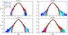 |
Fig. 1. PDFs of the SPI normalized by its standard deviation σ at different scales R, arising from four different turbulence regimes. The dashed black lines represent the Gaussian distributions. |
4. Synchrotron polarization simulation
4.1. Measurement of intermittency arising from different turbulence regimes
To generate the synthetic observations, we calculated the SPI via Equation (8) using the above data cubes, with the assumption of the thermal electron density ne proportional to the plasma density ρ, that is, ne = ρ when involving the Faraday rotation measure. We use the typical values of the Galactic ISM to parameterize dimensionless physical quantities. Here, we provide only three key parameters: the spatial length of L = 100 pc along the LOS, the thermal electron density  , and the magnetic field strength B = 1.23 μG. With the numerical resolution of 512 pixels, we had a mesh grid of 100 pc/512 ∼ 0.2 pc, corresponding to the smallest resolved spatial length.
We first analyzed the PDFs of SPI arising from four turbulence regimes (see Table 1). The resulting finding is shown in Fig. 1, where we see that the PDFs at different scales R exhibit other characteristics that deviate from the Gaussian distribution. In general, this deviation mainly occurs in the two tail parts of the Gaussian distribution. With the decreasing scale R, we found that the level of deviation from both tails increases (except for panel (a)), indicating intermittent enhancement. Comparing all four scenarios, the PDFs can qualitatively reveal the presence or disappearance of intermittency. Next, we quantitatively evaluated the intermittency level using kurtosis.
The kurtosis distributions of the SPI over the separation scale R are presented in Fig. 2, where the horizontal dashed line corresponds to K = 3, representing the kurtosis value of the Gaussian distribution shown in Fig. 1. As shown in Fig. 2, the kurtosis values of Run2 and Run3 decrease faster than those of Run1 and Run4 as the separation scale increases. This reflects the more obvious intermittency of both Run2 and Run3 at small scales. In other words, the greater the deviation from K = 3, the more the intermittency. The kurtosis of SPI shows an irregular coupling between the Mach numbers MA and Ms. Although there is intermittency at a small scale, we do not find a significant correlation between the kurtosis distribution and Mach numbers. However, it is apparent that the most intermittency corresponds to the largest deviations of β from unity.
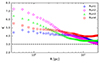 |
Fig. 2. Kurtosis of the SPI as a function of the separation scale R in different turbulence regimes. The horizontal dashed line corresponds to the kurtosis values of the Gaussian distribution. |
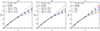 |
Fig. 3. Scaling exponent as a function of the order for the SPI at three scenarios: the lower limits of the fixed R (panel (a)), the upper limits of the fixed R (panel (b)), and different turbulence models (panel (c)). The results of panels (a) and (b) are obtained by Run2. |
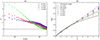 |
Fig. 4. Kurtosis (panel (a)) and scaling exponent (panel (b)) of the SPI at different frequencies for the simulation of Run1. The horizontal dashed line plotted in panel (a) corresponds to the kurtosis value of Gaussian distribution. |
In addition to the methods discussed above, the scaling exponent of multi-order structure functions is the third method for measuring intermittency. Specifically, we used the extended self-similarity (Benzi et al. 1993) to obtain the scaling exponent between the 3rd- and pth-order structure function. Here, we first explored how different fitting ranges for R affect the scaling exponent. Our results are shown in Fig. 3(a), which describes the relation between the scaling exponent and the order at different upper limits of the inertial range. In this figure, the dotted, dashed, and dash-dotted lines indicate theoretical results provided by the Kolmogorov, SL, and MB models, respectively. The error bar represents the standard deviation. From panel (a), we knew that different upper limits of the expected inertial range have little effect on the measurement of the scaling index, thus we fixed the separation scale R = 15.6 pc as an upper limit in Fig. 3(b). Similarly, Fig. 3(b) explores the influence of different lower limits of the approximate dissipation scale on the scaling index. It is clear that the distribution of ξ(p) with p behaves similarly, except for the results in the range of 0.2−15.6 pc. This may be affected by the numerical dissipation.
Based on the above exploration, we fixed the lower and upper limits of spatial scales as R = 0.6 and R = 15.6 pc, respectively. As is shown in Fig. 3(c), the scaling exponents in different turbulence regimes have different deviations from the Kolmogorov model. For Run1, namely the sub-Alfvénic and subsonic turbulence, the scaling exponent is close to being linear, revealing weak intermittency. For Run4, corresponding to the super-Alfvénic and supersonic case, we see that there is a significant deviation from the Kolmogorov model at the large order p, reflecting the presence of intermittency. For the other turbulence regimes (see Run2 and Run3), the distributions of the scaling exponent are fairly close to the SL model, characterizing greater intermittency.
4.2. Measurement of intermittency at different frequencies
Based on Run1, we explored the influence of frequency on the kurtosis and scaling exponent of the SPI, respectively. The numerical results are shown in Fig. 4, where in panel (a) we see that the frequency has a significant effect on the kurtosis profiles. At low frequencies, the kurtosis shows a dramatic rise toward the small scales, while at high frequencies, the kurtosis steadily increases over the small scales.
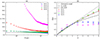 |
Fig. 5. Kurtosis (panel (a)) and scaling exponent (panel (b)) of Faraday rotation measure in different turbulence regimes. The horizontal dashed line plotted in panel (a) corresponds to the kurtosis value of the Gaussian distribution. |
This reflects that the intermittency at low frequencies becomes more significant than that at high frequencies, which may be due to the Faraday depolarization effect at low frequencies making more inhomogeneous structures. It can be seen that the most significant change in kurtosis occurs at the frequency of 0.4 GHz, indicating strong intermittency. Fig. 4(b) shows that the scaling exponent of SPI displays different behaviors at different frequencies. At the frequency of 0.4 GHz, there is an evident nonlinear relation close to the SL model. At the frequency of 0.5 GHz, the scaling exponent shows a slight departure from the Kolmogorov model, indicating weak intermittency. Moreover, the scaling index is close to a linear relation at high frequencies of 1.4 and 10 GHz, indicating weaker intermittency. As a result, the two methods consistently demonstrate that in the low-frequency range explored in this paper, the SPI statistics can probe the intermittency of magnetic turbulence.
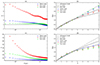 |
Fig. 6. Kurtosis (left column) and scaling exponent (right column) of the SPI for three modes. The results obtained by Run1 and Run2 are shown in the upper and lower rows, respectively. The horizontal dashed lines plotted in the left column correspond to the kurtosis values of the Gaussian distribution. |
4.3. Measurement of intermittency using Faraday rotation measure
The kurtosis of RMs as a function of the separation scale R is presented in Fig. 5(a), from which we see that there are large kurtosis values of RMs at a small R and small values at a large R. We also find that both supersonic turbulence cases (see Run2 and Run4) show much larger kurtosis values than the subsonic ones (Run1 and Run3). This reveals that the RMs in the supersonic turbulence regime are more intermittent than those in the subsonic one. The reason may be that the formation of shocks in the supersonic turbulence increases the intermittency of MHD turbulence. Among the four cases, the kurtosis values for Run2 are the largest, exhibiting the strongest intermittency.
Fig. 5(b) shows the scaling exponent for the RMs as a function of the order in the four different turbulence regimes. As shown in this panel, although all of the profiles show multi-fractal features, the scaling exponent ξ(p) varying with the order p behaves differently in different sonic turbulence regimes. In the subsonic turbulence regimes, the profile of ξ(p) almost follows the SL model, whereas in the supersonic turbulence regimes, it deviates far from the three theoretical models. This reveals that the RMs in supersonic turbulence regimes are more intermittent than those in the subsonic turbulence ones. Compared with three theoretical models, the scaling exponent in the sub-Alfvénic and supersonic turbulence regime displays the largest deviation, which reveals the greatest intermittency in this turbulence regime. Consequently, we find that the statistics of the Faraday rotation measure can recover the intermittency of MHD turbulence.
4.4. Measurement of intermittency of plasma modes
We first explored the kurtosis and scaling exponent for three plasma modes in the case of sub-Alfvénic and subsonic turbulence (i.e., Run1). The results are shown in the upper row of Fig. 6, in which panel (a) shows that the kurtosis of the Alfvén and slow modes decreases with the separation scale R, while that of the fast mode remains almost unchanged. Note that the kurtosis variations of the slow mode are the largest at small scales. This reflects the fact that the intermittency of the SPI in the sub-Alfvénic and subsonic turbulence regime is dominated by the slow mode. From Fig. 6(b), we see that the scaling exponents for the fast and slow modes follow the Kolmogorov and SL models, respectively, while for the Alfvén mode, the distribution of the scaling exponents lies in these two models. This may be related to the anisotropic level of the three modes in the sub-Alfvénic and subsonic turbulence regime. As demonstrated by Wang et al. (2020), the slow mode results in inhomogeneous structures because of its strong anisotropy, while the fast mode produces uniform fluctuations due to its isotropy. This suggests that the slow mode has the strongest intermittency, while the fast mode has no intermittency.
Moreover, the lower row of Fig. 6 explores the case of sub-Alfvénic and supersonic turbulence (i.e., Run2). Fig. 6(c) shows that the kurtosis of the SPI for the three modes exhibits different increasing levels as the separation scale decreases. It can be seen that the kurtosis of slow and fast modes shows a dramatic rise at small separation scales, while that of the Alfvén mode rises slowly. This indicates that the first two have stronger intermittency, while the latter does not manifest significant intermittency. This should be caused by the compressible nature of slow and fast modes in this turbulence regime. From Fig. 6(d), we see that the SPI for the three modes displays nonlinear scaling exponents. The scaling exponents for the Alfvén mode are consistent with the MB model, while those for the other two modes deviate from this model. As a consequence of these two methods, the SPI for the slow mode dominates the intermittency of MHD turbulence. In addition, compared with the results of Fig. 3(c), we find that the intermittency of the SPI for the post-decomposition MHD modes is stronger than that for the pre-decomposition MHD modes in the sub-Alfvénic and supersonic turbulence regime, which may be weakened by the coupling of the three modes.
CGPS archive data observed at  .
.
5. Application to observations
In this section, we explore the intermittency of the Galactic ISM using the archive data from the CGPS at 1.42 GHz1. The CGPS is a project involving radio, millimeter, and infrared surveys of the Galactic plane to provide arcminute-scale images of all major components of the ISM over a large part of the Galactic disk (Taylor et al. 2003). The synchrotron radio surveys are carried out at the Dominion Radio Astrophysical Observatory (DRAO). The DRAO Synthesis Telescope surveys imaged a 73° section of the Galactic plane between April 1995 and June 2000. The surveys cover the region with the longitude range of  and the latitude extent of
  . The full area of the CGPS is covered by 36 mosaics, each of which has a resolution of 1024 × 1024 pixels, corresponding to the
  region on the POS.
We explored the ISM turbulence intermittency by extracting the resolution of 512 × 512 pixels from the 1024 × 1024 mosaic image to avoid the margin of images. As a representative example, we firstly provided the PDFs from four mosaic images with the coordinate information listed in Table 2, as shown in Fig. 7. In practice, we filtered noise-like structures of data using a Gaussian kernel of σ = 2 pixels. From this figure, we can see that PDFs at different angle scales present different deviation levels of two tails from the Gaussian distribution. As the angle scale decreases, the deviation from the normal distribution increases, revealing an increment of intermittency. Moreover, we find that the PDFs in the four scenarios exhibit the presence of intermittency; however, which scenario has more abundant intermittency still needs to be further explored.
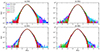 |
Fig. 7. PDFs of SPI are normalized by its standard deviation σ at different angles θ, arising from four sets of CGPS data. The dashed black lines represent the Gaussian distributions. |
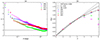 |
Fig. 8. Kurtosis (panel (a)) and scaling exponent (panel (b)) of the SPI for four sets of CGPS data at 1.42 GHz. The horizontal dashed line plotted in panel (a) corresponds to the kurtosis values of Gaussian distribution. |
Next, we quantitatively explored the degree of intermittency in the four scenarios. Fig. 8(a) depicts the kurtosis of SPI as a function of the separation angle for four sets of CGPS data. It can be seen that the kurtosis of SPI for MA2 and MC2 varies notably with the separation angle, while the kurtosis for MB2 and ME2 changes slowly. In this regard, we conclude that the SPI for MA2 and MC2 displays more intermittency than the SPI for MB2 and ME2. Fig. 8(b) presents the relation between the scaling exponent and order for the same datasets. It clearly shows that all of the curves of the scaling exponent are nonlinear, characterizing the presence of strong intermittency. For MB2 and ME2, the profiles of the scaling exponent coincide with those of MB model, while for MA2 and MC2, the scaling exponent deviates greatly from this model. This proves that the latter is more intermittent than the former. Compared with the results of the synthetic observations (see Section 4), we predict that the ISM around the Galactic plane corresponds to the sub-Alfvénic and supersonic regimes (Falceta-Gonçalves et al. 2008; Heyer et al. 2008; Burkhart et al. 2009).
6. Discussion
In this paper, we mainly explored the intermittency of MHD turbulence by the SPI and RM statistics. At sufficiently high frequencies, the SPI statistics can capture the intermittency of the projected magnetic fields B⊥ on the POS, while at low frequencies, the SPI statistics can provide insights into the intermittency properties of more physical quantities such as B∥, B⊥, and ne. At lower frequencies, the intermittency of the SPI can also be affected by the noise-like structures. On the other hand, the RM statistics can directly reflect the total intermittency for both ne and B∥, without involving the effect of B⊥. We also tested the contribution of ne and B∥ to the intermittency of RM separately, and found that the former contributes more than the latter.
We have utilized three common statistical methods – the PDFs, kurtosis, and scaling exponent of the multi-order structure function – to explore the intermittency of MHD turbulence. The PDFs act as an indicator for the presence of intermittency when they deviate from a Gaussian distribution. We note that this method can only qualitatively reflect the intermittency level at a certain separation scale. Differently, the kurtosis and scaling exponent can provide a quantitative estimation of intermittency. The kurtosis can display the intermittency over all of the separation scales. If the kurtosis varies faster with the separation scale, it implies that the fluid-structure is more intermittent. For the scaling exponent, when the relation between the scaling exponent and the order p becomes nonlinear, this indicates the multi-fractal feature of the fluctuations and the presence of intermittency. Our studies demonstrate that the results from the three methods explored are self-consistent, the synergy of which can provide a more comprehensive understanding of MHD turbulence intermittency.
This work was carried out in the framework of the modern understanding of MHD turbulence theory (Goldreich & Sridhar 1995). Considering that the magnetic field and velocity retain the same cascade properties, we used three theoretical models related to velocity, namely the Kolmogorov, SL, and MB models, to characterize the intermittency levels of magnetic turbulence. We also tested the intermittency of the 3D magnetic field and velocity and found that they have slightly stronger intermittency than that revealed by the SPI statistics. Therefore, we speculate that the measured intermittency should be slightly weaker than the underlying MHD turbulence intermittency. We think that the projection effect, that is, the integration along the LOS, attenuates the intrinsic intermittency amplitude of the Galactic ISM. Similarly, the direct numerical simulations also claimed that the 3D simulation shows more intermittency than the 2D one (e.g., Schmidt et al. 2008; Brunt et al. 2003; Brunt & Mac Low 2004); the 2D case is a projection from the 3D case.
Compared to the results from sub-Alfvénic and subsonic turbulence (see the upper panels of Fig. 6), our results demonstrate that in the case of sub-Alfvénic and supersonic (with the presence of shocks) turbulence (see the lower panels of Fig. 6), the intermittency of the solenoidal mode is intensified. At the same time, we also see the intensification of the intermittency of the compressive (slow and fast) modes. We emphasize that our results are obtained in the framework of solenoidal driving, which would cause more kinetic energy to be in solenoidal motions (e.g., Federrath et al. 2011). In any case, this finding suggests that shocks may be a source of intermittency.
Earlier studies claimed that the change in the spectral index only affects the amplitude of the structure function, which is only limited to the second-order structure function (Lazarian & Pogosyan 2016; Zhang et al. 2018). In this paper, we find that the change in the spectral index (α) affects not only the amplitude but also the scaling exponent for higher-order structures. As the spectral index increases, the intermittency of SPI becomes abundant. This is a new point. For the studies of other cases, we set the spectral index α = −1 for the calculation of SPI. Theoretically, one expects a bottleneck effect in the power spectra of the velocity and magnetic field at large wavenumbers. However, the power spectra obtained by our data cubes do not significantly show this effect (Wang et al. 2022; Kowal & Lazarian 2010). This effect does not influence the measurement of intermittency. However, the numerical dissipation at the smallest resolved spatial length 0.2 pc affects the results.
For our numerical studies, we provided the results up to the order p = 8. We find that with increasing order, the distributions of the scaling exponent are self-similar extending, that is, the increase in order did not change our numerical results. However, when we used the higher order (p > 12), there were significant fluctuations due to the limitation of the numerical resolution. For the realistic observational data, the maximum order of the structure function was only taken to the 6th order. When the 8th order is reached, the results will show abnormal fluctuations due to the de-noising of the real data.
Recently, the properties of MHD turbulence have been studied using the synchrotron polarization statistics (see Zhang & Wang 2022 for a recent review), including the spatial and frequency analysis techniques (Lazarian & Pogosyan 2016; Zhang et al. 2016; Lee et al. 2016), gradient techniques (e.g., Lazarian & Yuen 2018; Zhang et al. 2019), and quadrupole ratio modulus (Lee et al. 2019; Wang et al. 2020). We emphasize that these works focused mainly on the inertial range of the turbulence cascade. Differently, our work here covers a wide range of spatial scales, particularly involving the small-scale non-noise structure, in order to understand the properties of compressible MHD turbulence.
Cho & Lazarian (2010) proposed that analyzing intermittent features can separate foreground signals from cosmic microwave background signals via the high-order structure function. Intermittency can also explain the observed strong and rapid variations from pulsar magnetosphere (Zelenyi et al. 2015). We expect that measuring intermittency may distinguish the difference between the theories of Goldreich & Sridhar (1995) and Boldyrev (2006), which will be discussed elsewhere.
7. Summary
Using real observational data from the CGPS together with MHD turbulence simulation, we have investigated how to recover the intermittency of the magnetized ISM. The main results are briefly summarized as follows.
-
The SPI statistics can be used to probe the intermittency of MHD turbulence. The most significant intermittency appears in the sub-Alfvénic and supersonic turbulence regime, while the least intermittency appears in the sub-Alfvénic and subsonic one.
-
The intermittency measured by SPI depends on the level of the Faraday depolarization. The intermittency measured by RM shows a strong dependence on the sonic Mach number, with significant intermittency occurring in the supersonic turbulence regime. Therefore, the RM statistics can recover the intermittency of thermal electron density and magnetic field component along the LOS.
-
The slow mode dominates the intermittency of MHD turbulence in the sub-Alfvénic turbulence regime, where Alfvén (for supersonic) and fast (for subsonic) modes present almost negligible intermittency.
-
With the realistic observations from the CGPS, we find that the Galactic ISM at the low-latitude region corresponds to the sub-Alfvénic and supersonic turbulence regime.
The CGPS data is obtained from the Canadian Astronomy Data Centre: https://www.cadc-ccda.hia-iha.nrc-cnrc.gc.ca/en/cgps/
Acknowledgments
We would like to thank the anonymous referee for constructive comments that have significantly improved our manuscript. J.F.Z. is grateful for the support from the National Natural Science Foundation of China (Nos. 12473046 and 11973035), the Hunan Natural Science Foundation for Distinguished Young Scholars (No. 2023JJ10039), and the China Scholarship Council for the overseas research fund. F.Y.X. thanks the support from the National Natural Science Foundation of China (grant No. 12373024). R.Y.W. is grateful for the support from the Xiangtan University Innovation Foundation For Postgraduate (No. XDCX2022Y071).
References
- Anselmet, F., Hopfinger, E., & Antonia, R. 1984, J. Fluid Mech., 140, 63 [NASA ADS] [CrossRef] [Google Scholar]
- Beattie, J. R., Mocz, P., Federrath, C., & Klessen, R. S. 2022, MNRAS, 517, 5003 [NASA ADS] [CrossRef] [Google Scholar]
- Benzi, R., Ciliberto, S., Tripiccione, R., et al. 1993, Phys. Rev. E, 48, R29 [CrossRef] [Google Scholar]
- Beresnyak, A., & Lazarian, A. 2019, Turbulence in Magnetohydrodynamics (Walter de Gruyter GmbH& Co KG), 12 [CrossRef] [Google Scholar]
- Białas, A., & Seixas, J. 1990, Phys. Lett. B, 250, 161 [CrossRef] [Google Scholar]
- Biskamp, D. 2003, Magnetohydrodynamic Turbulence (Cambridge University Press) [Google Scholar]
- Boldyrev, S. 2006, Phys. Rev. Lett., 96, 115002 [Google Scholar]
- Bruno, R., Carbone, V., Sorriso-Valvo, L., & Bavassano, B. 2003, J. Geophys. Res.: Space Phys., 108, A3 [CrossRef] [Google Scholar]
- Bruno, R., D’Amicis, R., Bavassano, B., Carbone, V., & Sorriso-Valvo, L. 2007, Planet. Space Sci., 55, 2233 [NASA ADS] [CrossRef] [Google Scholar]
- Brunt, C. M., & Mac Low, M.-M. 2004, ApJ, 604, 196 [NASA ADS] [CrossRef] [Google Scholar]
- Brunt, C. M., Heyer, M. H., Vázquez-Semadeni, E., & Pichardo, B. 2003, ApJ, 595, 824 [NASA ADS] [CrossRef] [Google Scholar]
- Burkhart, B., Falceta-Gonçalves, D., Kowal, G., & Lazarian, A. 2009, ApJ, 693, 250 [Google Scholar]
- Butsky, I. S., Hopkins, P. F., Kempski, P., et al. 2024, MNRAS, 528, 4245 [NASA ADS] [CrossRef] [Google Scholar]
- Carbone, V., Bruno, R., Sorriso-Valvo, L., & Lepreti, F. 2004, Planet. Space Sci., 52, 953 [CrossRef] [Google Scholar]
- Chen, C. H. K., Sorriso-Valvo, L., Šafránková, J., & Němeček, Z. 2014, ApJ, 789, L8 [NASA ADS] [CrossRef] [Google Scholar]
- Chen, L. E., Bott, A. F. A., Tzeferacos, P., et al. 2020, ApJ, 892, 114 [NASA ADS] [CrossRef] [Google Scholar]
- Cho, J., & Lazarian, A. 2002, Phys. Rev. Lett., 88, 245001 [Google Scholar]
- Cho, J., & Lazarian, A. 2003, MNRAS, 345, 325 [NASA ADS] [CrossRef] [Google Scholar]
- Cho, J., & Lazarian, A. 2010, ApJ, 720, 1181 [NASA ADS] [CrossRef] [Google Scholar]
- Cho, J., Lazarian, A., & Vishniac, E. T. 2003, ApJ, 595, 812 [NASA ADS] [CrossRef] [Google Scholar]
- Davis, Z., Comisso, L., & Giannios, D. 2024, ApJ, 964, 14 [NASA ADS] [CrossRef] [Google Scholar]
- Décamp, N., & Malara, F. 2006, ApJ, 637, L61 [CrossRef] [Google Scholar]
- Esquivel, A., & Lazarian, A. 2010, ApJ, 710, 125 [NASA ADS] [CrossRef] [Google Scholar]
- Falceta-Gonçalves, D., Lazarian, A., & Kowal, G. 2008, ApJ, 679, 537 [Google Scholar]
- Falgarone, E., & Passot, T. 2008, Turbulence and Magnetic Fields in Astrophysics (Springer), 614 [Google Scholar]
- Falgarone, E., Godard, B., & Hily-Blant, P. 2011, in The Molecular Universe, eds. J. Cernicharo, & R. Bachiller, 280, 187 [NASA ADS] [Google Scholar]
- Federrath, C., Klessen, R. S., & Schmidt, W. 2008, ApJ, 688, L79 [NASA ADS] [CrossRef] [Google Scholar]
- Federrath, C., Klessen, R. S., & Schmidt, W. 2009, ApJ, 692, 364 [Google Scholar]
- Federrath, C., Roman-Duval, J., Klessen, R. S., Schmidt, W., & Mac Low, M. M. 2010, A&A, 512, A81 [NASA ADS] [CrossRef] [EDP Sciences] [Google Scholar]
- Federrath, C., Chabrier, G., Schober, J., et al. 2011, Phys. Rev. Lett., 107, 114504 [NASA ADS] [CrossRef] [Google Scholar]
- Fraternale, F., Pogorelov, N. V., Richardson, J. D., & Tordella, D. 2019, ApJ, 872, 40 [NASA ADS] [CrossRef] [Google Scholar]
- Frisch, U. 1995, Turbulence: the Legacy of AN Kolmogorov (Cambridge University Press) [CrossRef] [Google Scholar]
- Ginzburg, V. L., & Syrovatskii, S. I. 1965, ARA&A, 3, 297 [Google Scholar]
- Goldreich, P., & Sridhar, S. 1995, ApJ, 438, 763 [Google Scholar]
- Haugen, N. E., Brandenburg, A., & Dobler, W. 2004, Phys. Rev. E, 70, 016308 [NASA ADS] [CrossRef] [Google Scholar]
- Heyer, M., Gong, H., Ostriker, E., & Brunt, C. 2008, ApJ, 680, 420 [Google Scholar]
- Hily-Blant, P., Falgarone, E., & Pety, J. 2008, A&A, 481, 367 [NASA ADS] [CrossRef] [EDP Sciences] [Google Scholar]
- Huang, S. Y., Zhang, J., Yuan, Z. G., et al. 2022, Geophys. Res. Lett., 49, e96403 [NASA ADS] [Google Scholar]
- Kolmogorov, A. 1941, Akademiia Nauk SSSR Doklady, 30, 301 [Google Scholar]
- Kowal, G., & Lazarian, A. 2010, ApJ, 720, 742 [NASA ADS] [CrossRef] [Google Scholar]
- Kowal, G., Lazarian, A., & Beresnyak, A. 2007, ApJ, 658, 423 [Google Scholar]
- Lazarian, A., & Pogosyan, D. 2016, ApJ, 818, 178 [NASA ADS] [CrossRef] [Google Scholar]
- Lazarian, A., & Yuen, K. H. 2018, ApJ, 865, 59 [CrossRef] [Google Scholar]
- Lee, H., Lazarian, A., & Cho, J. 2016, ApJ, 831, 77 [NASA ADS] [CrossRef] [Google Scholar]
- Lee, H., Cho, J., & Lazarian, A. 2019, ApJ, 877, 108 [Google Scholar]
- Lemoine, M. 2021, Phys. Rev. D, 104, 063020 [NASA ADS] [CrossRef] [Google Scholar]
- Mallet, A., & Schekochihin, A. A. 2017, MNRAS, 466, 3918 [NASA ADS] [CrossRef] [Google Scholar]
- McKee, C. F., & Ostriker, J. P. 1977, ApJ, 218, 148 [NASA ADS] [CrossRef] [Google Scholar]
- Meneveau, C., & Sreenivasan, K. R. 1987, Phys. Rev. Lett., 59, 1424 [NASA ADS] [CrossRef] [Google Scholar]
- Müller, W.-C., & Biskamp, D. 2000, Phys. Rev. Lett., 84, 475 [CrossRef] [Google Scholar]
- Osman, K. T., Matthaeus, W. H., Greco, A., & Servidio, S. 2011, ApJ, 727, L11 [NASA ADS] [CrossRef] [Google Scholar]
- Osman, K. T., Matthaeus, W. H., Hnat, B., & Chapman, S. C. 2012a, Phys. Rev. Lett., 108, 261103 [NASA ADS] [CrossRef] [Google Scholar]
- Osman, K. T., Matthaeus, W. H., Wan, M., & Rappazzo, A. F. 2012b, Phys. Rev. Lett., 108, 261102 [NASA ADS] [CrossRef] [Google Scholar]
- Osman, K. T., Kiyani, K. H., Chapman, S. C., & Hnat, B. 2014, ApJ, 783, L27 [CrossRef] [Google Scholar]
- Phillips, C., Bandyopadhyay, R., McComas, D. J., & Bale, S. D. 2023, MNRAS, 519, L1 [Google Scholar]
- Rickett, B. 2011, AIP Conf. Ser., 1366, 107 [NASA ADS] [Google Scholar]
- Schmidt, W., Federrath, C., & Klessen, R. 2008, Phys. Rev. Lett., 101, 194505 [NASA ADS] [CrossRef] [Google Scholar]
- Servidio, S., Valentini, F., Califano, F., & Veltri, P. 2012, Phys. Rev. Lett., 108, 045001 [NASA ADS] [CrossRef] [Google Scholar]
- She, Z.-S., & Leveque, E. 1994, Phys. Rev. Lett., 72, 336 [Google Scholar]
- Taylor, A. R., Gibson, S. J., Peracaula, M., et al. 2003, AJ, 125, 3145 [NASA ADS] [CrossRef] [Google Scholar]
- Vega, C., Boldyrev, S., & Roytershteyn, V. 2023, ApJ, 949, 98 [NASA ADS] [CrossRef] [Google Scholar]
- Veltri, P. 1999, Plasma Phys. Controlled Fusion, 41, A787 [NASA ADS] [CrossRef] [Google Scholar]
- Vincent, A., & Meneguzzi, M. 1991, J. Fluid Mech., 225, 1 [NASA ADS] [CrossRef] [Google Scholar]
- Wan, M., Osman, K. T., Matthaeus, W. H., & Oughton, S. 2012, ApJ, 744, 171 [NASA ADS] [CrossRef] [Google Scholar]
- Wang, Y., Wei, F. S., Feng, X. S., et al. 2015, ApJS, 221, 34 [NASA ADS] [CrossRef] [Google Scholar]
- Wang, R.-Y., Zhang, J.-F., & Xiang, F.-Y. 2020, ApJ, 890, 70 [NASA ADS] [CrossRef] [Google Scholar]
- Wang, R.-Y., Zhang, J.-F., Lazarian, A., Xiao, H.-P., & Xiang, F.-Y. 2022, ApJ, 940, 158 [NASA ADS] [CrossRef] [Google Scholar]
- Wu, P., Perri, S., Osman, K., et al. 2013, ApJ, 763, L30 [NASA ADS] [CrossRef] [Google Scholar]
- Xu, S. B., Huang, S. Y., Yuan, Z. G., et al. 2023, Geophys. Res. Lett., 50, e2023GL104656 [NASA ADS] [CrossRef] [Google Scholar]
- Yang, L., Zhang, L., He, J., et al. 2018, ApJ, 855, 69 [NASA ADS] [CrossRef] [Google Scholar]
- Yoshimatsu, K., Schneider, K., Okamoto, N., Kawahara, Y., & Farge, M. 2011, Phys. Plasmas, 18, 9 [CrossRef] [Google Scholar]
- Zelenyi, L. M., Bykov, A. M., Uvarov, Y. A., & Artemyev, A. V. 2015, J. Plasma Phys., 81, 395810401 [NASA ADS] [CrossRef] [Google Scholar]
- Zhang, J.-F., & Wang, R.-Y. 2022, Front. Astron Space Sci., 9, 869370 [NASA ADS] [CrossRef] [Google Scholar]
- Zhang, J.-F., Lazarian, A., Lee, H., & Cho, J. 2016, ApJ, 825, 154 [NASA ADS] [CrossRef] [Google Scholar]
- Zhang, J.-F., Lazarian, A., & Xiang, F.-Y. 2018, ApJ, 863, 197 [NASA ADS] [CrossRef] [Google Scholar]
- Zhang, J.-F., Liu, Q., & Lazarian, A. 2019, ApJ, 886, 63 [NASA ADS] [CrossRef] [Google Scholar]
- Zhdankin, V., Boldyrev, S., & Chen, C. H. K. 2016, MNRAS, 457, L69 [NASA ADS] [CrossRef] [Google Scholar]
Appendix A: Multi-order structure functions
In this appendix, we provide the multi-order structure functions of the SPI and RM in Figs. A.1 and A.2, respectively. These figures exhibit the structure functions with different orders as a function of SF3(R). As is shown in these figures, we can see a good power-law relation. For quantitative characterization, we perform a linear fitting process in the interval between R = 0.6 and R = 15.6 pc. According to the fitting from these two figures, we can further obtain the results of Figs. 3(c) and 5, respectively, where the uncertainties arising from the linear fitting are reflected by the error bars, i.e., the standard deviations.
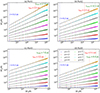 |
Fig. A.1. Structure functions of the SPI with different orders (from p = 1 to 8) as a function of SF3(R) under the extended self-similarity hypothesis. The vertical blue, green, and red dotted lines denote the values of third-order structure function in the smallest resolved spatial length, transition scale, and dissipation scale, respectively. The black dashed lines show a linear fit to the structure function on log-log scales. |
All Tables
All Figures
|
Fig. 1. PDFs of the SPI normalized by its standard deviation σ at different scales R, arising from four different turbulence regimes. The dashed black lines represent the Gaussian distributions. |
| In the text | |
|
Fig. 2. Kurtosis of the SPI as a function of the separation scale R in different turbulence regimes. The horizontal dashed line corresponds to the kurtosis values of the Gaussian distribution. |
| In the text | |
|
Fig. 3. Scaling exponent as a function of the order for the SPI at three scenarios: the lower limits of the fixed R (panel (a)), the upper limits of the fixed R (panel (b)), and different turbulence models (panel (c)). The results of panels (a) and (b) are obtained by Run2. |
| In the text | |
|
Fig. 4. Kurtosis (panel (a)) and scaling exponent (panel (b)) of the SPI at different frequencies for the simulation of Run1. The horizontal dashed line plotted in panel (a) corresponds to the kurtosis value of Gaussian distribution. |
| In the text | |
|
Fig. 5. Kurtosis (panel (a)) and scaling exponent (panel (b)) of Faraday rotation measure in different turbulence regimes. The horizontal dashed line plotted in panel (a) corresponds to the kurtosis value of the Gaussian distribution. |
| In the text | |
|
Fig. 6. Kurtosis (left column) and scaling exponent (right column) of the SPI for three modes. The results obtained by Run1 and Run2 are shown in the upper and lower rows, respectively. The horizontal dashed lines plotted in the left column correspond to the kurtosis values of the Gaussian distribution. |
| In the text | |
|
Fig. 7. PDFs of SPI are normalized by its standard deviation σ at different angles θ, arising from four sets of CGPS data. The dashed black lines represent the Gaussian distributions. |
| In the text | |
|
Fig. 8. Kurtosis (panel (a)) and scaling exponent (panel (b)) of the SPI for four sets of CGPS data at 1.42 GHz. The horizontal dashed line plotted in panel (a) corresponds to the kurtosis values of Gaussian distribution. |
| In the text | |
|
Fig. A.1. Structure functions of the SPI with different orders (from p = 1 to 8) as a function of SF3(R) under the extended self-similarity hypothesis. The vertical blue, green, and red dotted lines denote the values of third-order structure function in the smallest resolved spatial length, transition scale, and dissipation scale, respectively. The black dashed lines show a linear fit to the structure function on log-log scales. |
| In the text | |
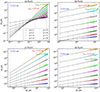 |
Fig. A.2. Same as Fig. A.1, but for the multi-order structure functions of the RM statistics. |
| In the text | |
Current usage metrics show cumulative count of Article Views (full-text article views including HTML views, PDF and ePub downloads, according to the available data) and Abstracts Views on Vision4Press platform.
Data correspond to usage on the plateform after 2015. The current usage metrics is available 48-96 hours after online publication and is updated daily on week days.
Initial download of the metrics may take a while.