| Issue |
A&A
Volume 672, April 2023
|
|
|---|---|---|
| Article Number | A152 | |
| Number of page(s) | 20 | |
| Section | The Sun and the Heliosphere | |
| DOI | https://doi.org/10.1051/0004-6361/202243034 | |
| Published online | 14 April 2023 | |
Simulating Rayleigh-Taylor induced magnetohydrodynamic turbulence in prominences⋆
Centre for mathematical Plasma-Astrophysics, Celestijnenlaan 200B, 3001 Leuven, KU Leuven, Belgium
e-mail: This email address is being protected from spambots. You need JavaScript enabled to view it.
Received:
3
January
2022
Accepted:
7
February
2023
Abstract
Aims. Solar prominences are large-scale condensations suspended against gravity within the solar atmosphere. The Rayleigh-Taylor (RT) instability is proposed to be one of the fundamental processes that lead to the generation of dynamics at many spatial and temporal scales within these long-lived, cool, and dense structures, which are located in the solar corona. We aim to study such turbulent processes using high-resolution, direct numerical simulations of solar prominences.
Methods. We ran 2.5D ideal magnetohydrodynamic (MHD) simulations with the open-source MPI-AMRVAC code far into the nonlinear evolution of an RT instability perturbed at the prominence-corona interface. Our simulation achieves a resolution down to ∼23 km on a 2D (x, y) domain of size 30 Mm × 30 Mm. We followed the instability transitioning from a multimode linear perturbation to its nonlinear, fully turbulent state. Over the succeeding ∼25 min period, we performed a statistical analysis of the prominence at a cadence of ∼0.858 s.
Results. We find that the dominant guiding component, Bz, induces coherent structure formation predominantly in the vertical velocity component, Vy, consistent with observations, indicating an anisotropic turbulence state within our prominence. We find power-law scalings in the inertial range for the velocity, magnetic, and temperature fields. The presence of intermittency is evident from the probability density functions of the field fluctuations, which depart from Gaussianity as we consider smaller and smaller scales. In exact agreement, the higher-order structure functions quantify the multi-fractality, as do different scale characteristics and the behavior between the longitudinal and transverse directions. Thus, the statistics remain consistent with conclusions from previous observational studies, enabling us to directly relate the RT instability to the turbulent characteristics found within quiescent prominences.
Key words: magnetohydrodynamics (MHD) / Sun: filaments / prominences / Sun: atmosphere / methods: numerical / instabilities / turbulence
Movie is available at https://www.aanda.org
© The Authors 2023
 Open Access article, published by EDP Sciences, under the terms of the Creative Commons Attribution License (https://creativecommons.org/licenses/by/4.0), which permits unrestricted use, distribution, and reproduction in any medium, provided the original work is properly cited.
This article is published in open access under the Subscribe to Open model. This email address is being protected from spambots. You need JavaScript enabled to view it. to support open access publication.
1. Introduction
Solar prominences are large structures that contain relatively cool (104 K) and dense condensations embedded within the far hotter (106 K), tenuous solar corona. The characteristic dimensions of prominences range from 60 to 600 Mm in length, 15 to 100 Mm in height, and 5 to 15 Mm in thickness (Tandberg-Hanssen 1995). They are mainly classified into three types, active, intermediate, and quiescent, based on their lifetime, location on the Sun, and strength of the interrelated magnetic field (Mackay et al. 2010). They originate from filament channels and develop above magnetic polarity inversion lines (the observed delineation between predominantly positive and negative fields at photospheric heights). Quiescent prominences are usually found in quiet regions in the Sun’s atmosphere, at a range of latitudes, and populate the largest of the aforementioned scales.
A typical quiescent prominence exists within quiet regions of the solar corona with an electron number density ∼1011 cm−3 (Hirayama 1986) and temperatures around ∼104 K (Tandberg-Hanssen 1995). According to early observations, the internal magnetic field is mostly horizontal to the solar surface, making an acute angle of about 40° with respect to the long axis of the prominence (Bommier & Leroy 1998). With the exception of Merenda et al. (2006), who found a nearly vertical field orientation, the majority of subsequent works continue to find evidence of a horizontally oriented internal magnetic field of magnitude a few tens of gauss and a slightly broader range of thread deviation angles (> 15°) from the guiding axis (Collados et al. 2003; Casini et al. 2003; Levens et al. 2016).
Initially, Rust (1967) estimated the plasma β ratio, the thermal to magnetic pressure, to be ≈0.02. Such a low β in prominences means that the Lorentz force, particularly the magnetic tension component, must be responsible for supporting the prominence material; the key force balance for such a magneto-hydrostatic equilibrium then is magnetic tension and gravity. Zhou et al. (2021) discussed the relative importance of the key forces in prominence dynamics. Most notably, gravity can be dynamically essential in prominences even for β < 1, if the system size is larger than the pressure scale height. For quiescent prominences, more recent studies have found the pressure and magnetic field strength values to be on the order of ≈0.1 dyne cm−2 and 10 G, respectively, increasing to as much as 0.4 – 0.6 dyne cm−2 and 60 – 80 G (for both quiescent and active environments; Hirayama 1986; Casini et al. 2003; Luna et al. 2018; Schwartz et al. 2019). Hence, since the initial plasma beta estimates of Rust (1967), this further research enables us to conclude that the range of plasma β within prominences can be across four orders of magnitude, ranging from 0.0004 – 4. Naturally, this has major implications for the range of plasma dynamics to be found within solar prominences.
Detailed observations of these phenomena have shown a spatio-temporal range of internal dynamics, curiously dominated by many vertical striations (Berger et al. 2008). These prominence plumes are observed as dark, rising voids in cool spectral lines. The upflowing plumes measured by the Hinode Solar Optical Telescope (SOT) and analyzed by Berger et al. (2010) were found to have characteristic initial widths of 0.5 to 1.7 Mm. These structures appear to rise with near-constant speeds of 10 to 17 km s−1, have areal dimensions between 2 and 6 Mm, and reach a maximum height of 11 to 17 Mm, before eventually descending as pillars with an acceleration of 0.48 to 3.2 km s−2. Berger et al. (2010), Ryutova et al. (2010), Innes et al. (2012), and Mishra & Srivastava (2019) propose that the Rayleigh-Taylor (RT) instability may be a key mechanism for driving upflow plumes and descending pillars. It is a fundamental instability driven by gravity, where a heavier fluid is accelerated against a lighter fluid separated by an interface that is unstable to perturbations. In an ideal, stratified magnetohydrodynamic (MHD) model, a discontinuous interface between the heavier and lighter fluids is similarly unstable to such perturbations. The deposition of hydrodynamic baroclinic vorticity therein amplifies initial deformations of the interface as a result of the misalignment between the local pressure and density gradients (Zhou et al. 2021), with the linear growth rate then increasing with increasing mode number (Chandrasekhar 1961).
The high-resolution observations from Hinode SOT are largely responsible for our understanding of the nonlinear behavior of the internal dynamics of quiescent prominences (Chae 2010; Hillier et al. 2012a). Chae (2010) found from the observations that the vertical fine substructures, termed knots, were impulsively accelerated in the downward direction. The authors related this to magnetic reconnection and the interchange of the magnetic configuration. The SOT observations of Berger et al. (2008, 2010) and Berger et al. (2011) additionally linked these dynamics to the aforementioned magnetic RT instability, as well as to the well-known Kelvin-Helmholtz (KH) instability, and this was subsequently validated in numerical works (Hillier et al. 2011, 2012a). Naturally, these earlier studies focused on the velocity field, specifically this wide range of motions in the vertical direction (Engvold 1981; Kubota & Uesugi 1986), and highlighted, importantly, how these upflows subsequently evolve into vortices (Liggett & Zirin 1984). Furthermore, the upward flows can be supersonic, and evidence of bow-shock compression is reported by Berger et al. (2010). And so, in general, quiescent prominences are seen to exhibit spatio-temporal evolution characterized by high variability. The dynamic nature and the large prevailing Reynolds numbers then indicate that the fluctuations present within prominences are turbulent in nature.
Following such conclusions, Leonardis et al. (2012) used the Ca II H intensity images from Hinode SOT to explore the quantitative signatures of turbulence related to solar prominences for the first time. The authors looked at the turbulence non-Gaussianity, multi-fractality, and intermittency aspects, studying the power-law scalings within the power spectral density (PSD) as a function of wavenumber. From this, Freed et al. (2016) also used Hinode SOT data to investigate the characteristics of the plasma flow, focusing primarily on the kinetic energy and vorticity. Shortly after that, Hillier et al. (2017) used Hα Dopplergrams from Hinode SOT to investigate the nature of turbulent prominence motions, applying structure function (SF) analysis to the velocity increments. In this paper we use direct numerical simulations and analyze our MHD model of a quiescent prominence in much the same fashion as in these previous studies.
Theoretical studies using ideal MHD simulations have been carried out by Hillier et al. (2012a,b), Keppens et al. (2015), and Xia & Keppens (2016a), who were able to reproduce upflows and downflows with speeds consistent with observational values. Hillier et al. (2012a,b) performed 3D MHD simulations of the RT instability mode development in the lower regions of prominence boundaries to investigate the nonlinear stability of the Kippenhahn-Schlüter model (Kippenhahn & Schlüter 1957). A total of 40 × 150 × 320 (x × y × z) grid points were used in this 3D numerical simulation. The nonlinear RT instability formed low-density filamentary structures aligned in the magnetic field direction, which was important for creating upflows in the prominence. In Keppens et al. (2015), the macroscopic behavior of the RT instability and its ability to form bubbles and pillars were studied using 3D ideal-MHD simulations. In that study, a resolution of 600 × 600 × 280 was achieved using dynamic grid refinement to simulate the late nonlinear stages for a weak field case of 8 G. The study shows the development of substructures along the edges of the largest bubbles in the system, in line with the existence of strong shear flows previously noted from observations. These various studies mainly focused on the evolution of the early nonlinear RT stages (up to a saturation regime) in a quiescent prominence. However, the study of the ensuing, persistent turbulence has been limited so far.
Terradas et al. (2015) used 3D MHD simulations of global prominence models to investigate and relate the prominence morphology and dynamics to the different model parameters. Investigating the time evolution of solar prominences embedded in sheared magnetic arcades, the authors demonstrated that magnetic shear and low plasma β stabilize the configuration. The Terradas et al. (2015) study was performed using a resolution of 150 × 150 × 100. The setup had no initial velocity perturbation, but due to ad hoc mass deposition, the system generated vertical velocity perturbations as mass got pulled down by gravity. The flows in Terradas et al. (2015) are due to gravitational potential energy leading to the formation of RT instability-like dynamics; the coarse resolution prevented direct comparisons against observed scales. Using 3D MHD simulations, Terradas et al. (2016) then continued with a study of the temporal evolution of a cold solar prominence embedded in a 3D magnetic flux rope, where the orientation of the prominence along the flux rope axis prevented the development of the RT instability altogether.
More recently, Xia & Keppens (2016b) used 3D MHD simulations to investigate the nonlinear magneto-convective motions within a twin-layer prominence beginning with a predominantly horizontal magnetic field and a gravitationally force-balanced solar atmosphere. To do so, a box of 30 × 30 × 30 Mm with a grid resolution of 600 × 600 × 600 with the smallest grid cell size of 50 km was taken. The initial evolution of the two layers is very similar due to the supporting magnetic field, which becomes interchanged due to the RT instability. This similarity decreases in the later turbulent phase, and, as a collective kink, deformation was induced in the twin-layer prominence. Kaneko & Yokoyama (2018) performed high-resolution 3D MHD modeling of the RT instability in prominences, which was able to reproduce magnetic RT dynamics within a prominence formed pseudo ab initio via the reconnection-condensation model. As an initial condition, the necessary perturbations were added to density and velocity in this study, resulting in a heterogenous radiative condensation. Interestingly, the condensation rate found was comparable to the mass drainage rate, meaning the total mass of the prominence was maintained. Unlike in Keppens et al. (2015), where the domain had a transition region above the lower chromosphere boundary, which resulted in the reflection of material from falling spikes due to the RT instability to then rise to coronal heights, Kaneko & Yokoyama (2018) used a full coronal domain. For a more detailed explanation of RT instability in prominences, the reader is directed to Hillier (2018) and Jenkins & Keppens (2022), who advocate for a timely migration toward generality through the gravitational interchange instability.
In summary, each of the abovementioned studies sfocused mostly on the early linear and nonlinear stages of RT instability in prominences using a wide array of models that differed significantly in terms of complexity. To clearly understand whether the RT instability could be a key factor leading to the turbulence observed in prominences, a physically detailed and long-duration run of the simulation is needed. The derived statistics should then be compared directly to observations. Furthermore, and based on the results presented by all of the above authors, it is clear that a yet-higher resolution is required to capture the smaller scales of the instability and any resulting turbulence, without which the dynamics at these scales will be dominated by numerical diffusion. The RT instability growth will be limited to the earlier, larger-scale evolutions.
Analytical and numerical studies of the RT instability in solar prominences are mostly carried out using the single-fluid MHD approach. A limited number of numerical studies using the ambipolar term to characterize partial ionization effects have been carried out for flux emergence (Arber et al. 2007; Martínez-Sykora et al. 2015) and for prominences (Díaz et al. 2014; Khomenko et al. 2014). In the context of more complete two-fluid approaches, numerical work regarding solar prominences are far scarcer. Díaz et al. (2012) used a two-fluid approach to study the linear onset and growth rate of the RT instability within the partially ionized plasma. Recent works of Popescu Braileanu et al. (2021a,b) have used a nonlinear two-fluid model to study the effects of partial ionization on the growth rate of the RT instability. The authors find the deviation from MHD to be important only at extremely small scales, around ∼3 km. The ambipolar term and true two-fluid treatments indeed affect the growth of small scales. Still, here we ignore the effects of plasma-neutral couplings in our simulation, which can be a topic for future investigation. Here, using the ideal MHD approach, we deal with scales above 20 km to understand the scale dependence on the turbulence previously observed in solar prominences due to the RT instability. At these scales, a single fluid MHD description suffices.
This work presents the first study of high-resolution simulated turbulence initiated by the RT instability within a 2.5D solar prominence (cf. Popescu Braileanu et al. 2021c). We have divided our paper into two sections. First, in Sect. 2, we discuss how we set up the numerical simulation, that is, the governing equations and initial and boundary conditions, to represent a 2.5D ideal MHD prominence unstable to the RT instability. We discuss the evolution of this instability from a linear phase to a nonlinear phase and finally to a turbulent phase, where the energy transfer through the intermediate scales takes place. Then, in Sect. 3, we analyze the turbulence in our simulated prominences with different field strengths and discuss the statistical methods that help us understand the prominence turbulence features. Finally, we present our summary and conclusions in Sect. 4.
2. Numerical setup
To investigate the characteristics of turbulence induced due to the RT instability, we performed 2.5D high-resolution ideal MHD simulations of a quiescent prominence in the solar atmosphere using the parallelized, open-source Adaptive Mesh Refinement Versatile Advection Code (MPI-AMRVAC; Keppens et al. 2012, 2021; Porth et al. 2014; Xia et al. 2018). It is a parallel adaptive mesh refinement (AMR) code that solves (primarily hyperbolic) partial differential equations using conservative variables (density, momentum density, total energy density, and magnetic field) across a finite volume grid. We chose a 2.5D setup to simplify the problem analytically and computationally, representing an efficient way of resolving the small scales for the turbulent study of solar prominences using the ideal MHD model. The 2.5D nature implies that we have velocity and magnetic field components perpendicular to the simulated (x, y) plane, and invariance is assumed along the z direction. We set up a large simulation domain using cartesian geometry, spanning 30 Mm horizontally along the solar surface and 30 Mm in height extending from the photosphere – low chromosphere into the solar corona. We adopt a base grid resolution of 40 × 40 and use a maximum refinement level of six to achieve a final grid resolution of 1280 × 1280. This is represented by the time evolution of the AMR grid level in Fig. 1, where the number of grids per AMR level is shown. It starts from the base grid AMR level 0 and goes until the highest AMR level 5. This figure shows an order of magnitude change in the coverage at the highest (most expensive) AMR level, which translates into an instant corresponding reduction in compute time. The final 600 seconds or so then cost exactly the same as a uniform grid resolution run. As we intend to study and quantify turbulence in a dynamically evolving, stratified prominence setup, the use of AMR allows efficient computation of the transition to a more volume-filling turbulent state and saves appreciable computing resources compared to employing a uniform mesh at 1280 × 1280 at all times. This is characterized by the highest level grid domain coverage percentage, which climbs from 59.44% at t = 0 s to nearly 100% by t = 420 s.
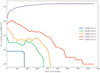 |
Fig. 1. Number of grids per AMR level during the evolution of the flow. |
We note that the observational study of Leonardis et al. (2012) on the turbulent characteristics of intensity fluctuations in prominences used intensity images obtained from the Hinode spacecraft, which gave a spatial resolution of ∼77.22 km with an average temporal resolution of 16.8 s for a total time interval of ∼4.5 hours. Each image consisted of 800 × 400 pixels. We achieve a higher spatial resolution of ∼23 km and base our analysis on data with a temporal resolution of 0.858 s for a total time interval of ∼25 minutes.
2.1. Governing equations
We solved the ideal MHD equations of conservation of mass, momentum, total energy density, and induction by using the MPI-AMRVAC code. The equations are given by
 (1)
(1)
 (2)
(2)
 (3)
(3)
 (4)
(4)
where p = (γ − 1)(e − ρv2/2 − B2/2) and ptot = p + B2/2, the quantities ρ, v, p, ptot, e, and B denote density, velocity vector, plasma pressure, total pressure, total energy density, and magnetic field vector, respectively, and γ (adiabatic index) is the ratio of specific heats, taken as 5/3 under the assumption of a monatomic ideal gas. The magnetic field vector is measured in units for which magnetic permeability equals μ0 = 1. The plasma temperature, T, is defined with the ideal gas law,
 (5)
(5)
where R and μ are the gas constant and mean molecular mass, respectively. We set up the following normalization quantities of unit length = 1 × 109 cm, unit temperature = 1 × 10⁶ K, unit number density = 1 × 109 cm−3 in our code. Equivalently in code units, the unit velocity is 1.16 × 107 cm s−1, the unit mass is 2.34 × 10¹² g, the unit density is 2.34 × 10⁻¹⁵ g cm−3, and the unit time is 85.87 s. The constant gravitational acceleration is then formulated as dimensionless according to the magnitude at the solar surface,  , in the y direction.
The Eqs. (1)–(4) are solved on an evolving, hierarchical block-adaptive grid, using a four−stage, third−order Runge-Kutta method (Ruuth & Spiteri 2002), with the Harten-Lax-van-Leer approximate Riemann solver for multiple discontinuities (HLLD; Miyoshi & Kusano 2005) and using a third-order asymmetric slope limiter given by Koren (1993). The HLLD method is a positivity-preserving method designed to resolve high-resolution MHD evolutions more robustly and gives higher efficiency than linearized Riemann solvers with respect to numerical accuracy. To ensure we achieve a stable state of turbulence, we use refinement criteria based on instantaneous plasma properties and their gradients, at the current time step following Lohner’s prescription. We used the generalized Lagrange multiplier (GLM) method (Dedner et al. 2002) for the magnetic field divergence fix, where the divergence constraint is coupled with the conservation laws by introducing an additional scalar variable, ψ. We adopted a Courant value of 0.8 to ensure a stable time step within the explicit time integration of each iteration.
2.2. Initial and boundary conditions
The 2D simulation domain was initialized at t = 0 on 0 ≤ x ≤ 30 Mm and 0 ≤ y ≤ 30 Mm. The bottom of the initial, purely inserted prominence lies at yb = 11.25 Mm, and the prominence transitions to the outer corona starting at yp = 17.5 Mm. The mean magnetic field strength is taken to be around 4 G. The initial magnetic field is taken as B = (0.1G, 0, Bz(y)), which is a purely 1D stratified profile, taken to be nonuniform with an exponential decrease of its strongest component Bz(y) between a height of yb and yp. The magnetic field makes an angle (θ) of ∼ 88.5° with the horizontal x-axis, so it is nearly perpendicular to the simulated plane. The exact analytic form of Bz(y) is given by
![Mathematical equation: $$ \begin{aligned} B_z = {\left\{ \begin{array}{ll} B_{z0},&{ y} < { y}_b\\ B_{z0} \exp \Bigg [- \left({ y}-{ y}_b\right)/ \lambda _B\Bigg ],&{ y}_b \leqslant { y} \leqslant { y}_p\\ B_{z0} \exp \Bigg [- \left({ y}_p-{ y}_b\right)/ \lambda _B\Bigg ],&{ y}_p < { y} , \end{array}\right.} \end{aligned} $$](/articles/aa/full_html/2023/04/aa43034-22/aa43034-22-eq7.gif) (6)
(6)
where the parameters are Bz0 = 4 G and pressure scale-height, λB = 15 Mm. Within the transition region between yb and yp, the Lorentz force ((∇ × B)×B) is not zero, which leads to the magnetic field configuration in the region being non-force-free. In the presence of gravity, the governing equation for magneto-static equilibrium becomes
 (7)
(7)
which constitutes the vertical force balance between the pressure, Lorentz force, and gravity of the plasma in the prominence material. A decrease in the magnetic field strength within the body of the prominence establishes an upward magnetic pressure force holding the prominence material against the gravity force in the solar atmosphere while also inducing a continuous shear due to the rotating magnetic field.
The initial vertical equilibrium, including the chromosphere, a coronal part below the prominence, the prominence, and the corona above, is thus set up by first initializing a magneto-hydrostatic equilibrium from the vertical temperature profile as shown in Fig. 2 and given by
 (8)
(8)
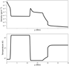 |
Fig. 2. Derived density (top) and enforced initial temperature (bottom) profiles in the vertical direction at the initial state. The temperature is set to be 8000 K in the chromosphere and transitions to 1.8 × 10⁶ K for the corona, dropping at y = yb to 6000 K for the lower part of the prominence. It then has a linear increasing profile from 6000–14 000 K at y = yp to y = 20 Mm for the upper part of the prominence. |
where the y values are in Mm, Tch is the temperature of the chromosphere = (8 × 10³), Tco of the corona = (1.8 × 10⁶), Tpromin is the minimum temperature of the prominence= = (6 × 10³) and Tpromax is the maximum temperature of the prominence = (1.4 × 10⁴). This sets a temperature of 8000 K in the chromosphere, transitioning to 1.8 × 10⁶ K for the corona, dropping at y = yb to 6000 K for the lower part of prominence and an increasing linear profile from 6000 to 14 000 K for the upper part of the prominence ending at 20 Mm. The different temperature regions in the vertical direction of the stratified solar atmosphere are connected smoothly using a hyperbolic tangent function. Then, the corresponding gas pressure and density stratifications are derived, ensuring magneto-hydrostatic balance as expressed in Eq. (7). Under the assumption of a fully ionized plasma with a 10:1 abundance ratio of H: He,  , we have the relation ρ = 1.4mpnH, where mp is the proton mass and nH the number density of hydrogen. Up to heights y = yb, we simply compute the 1D pressure and density array at an arbitrarily high resolution from the ideal gas law combined with the discrete formula,
 (9)
(9)
where gj is the local solar gravity value given as  cm s−2 and j is a grid index along the vertical direction. For y > yb, a similar formula is used where the Lorentz force is additionally accounted for. The Bz field, in this case, is defined by the following formula,
 (10)
(10)
and we solve the corresponding pressure as in Eq. (9), which is given as follows,
 (11)
(11)
The self-consistently derived density profile corresponding to the prescribed temperature stratification is then shown in Fig. 2. The simulation parameters thus represent conditions typical to a quiescent prominence. From a modeling perspective, the most relevant aspect of capturing prominence dynamics is to adopt the right density and temperature contrast realized in prominences while allowing for a fully gravitationally stratified atmosphere in a magnetized environment. Our initial conditions match these contrasts and adopt a temperature stratification (in line with previous model efforts as in Keppens & Xia 2014). The two-order of magnitude density inversion present at the prominence lower edge matches that extensively studied in earlier local box studies (Hillier et al. 2012a,b; Keppens et al. 2015; Xia & Keppens 2016a; Terradas et al. 2016). The adopted magnetic field is weak (4G), and at the lower edge of the quiescent prominence range, but we note that the pressure is derived from the magneto-hydrostatic equilibrium. The more important dimensionless parameter called plasma β is shown as a function of height at different times in our later Fig. 3. Most of the time, but especially during the initial stages, we remain below unity throughout the corona. We note that values up to plasma beta unity and above are reported in various works on prominences (see the review in Gibson 2018). Our t = 0 model ingredients are in accord with current understandings from ideal MHD modeling.
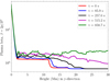 |
Fig. 3. Local plasma beta (averaged in the x direction) in the initial prominence of the reference case θ = 88.5° at t = 0 s (red) compared to its evolution in time at t= 85.9 s, 257.6 s, 515.2 s, and 858.7 s. |
The boundary conditions are set to be periodic on the left and right sides, and the top and bottom boundary conditions were specially handled in the simulation setup. The boundary values at the bottom were fixed for all time steps; for the top boundary, we extrapolate the density and pressure from the inner cells assuming hydrostatic equilibrium. In contrast, the magnetic field is extrapolated assuming zero normal gradients, and the velocity values are copied from the inner cells into the ghost cells.
The region of higher density in the corona mimics our prominence body, extending from the lower prominence corona transition region at yb = 11.25 Mm up to a height of 20 Mm. We initiate the RT instability by inducing a multimode perturbation within the lower prominence-corona interface. This perturbation is a superposition of 50 small-amplitude sinusoidal velocity fields, periodic in the x direction with random phases. As the initial condition is unstable, the perturbation will deform the interface to form bubbles and pillars. The resulting mixing in the presence of the mean magnetic field is dependent on the angle between the perturbation wave vector k and the mean magnetic field B, where the tension of the field can suppress the growth of the instability. This effect was first studied analytically by Chandrasekhar (1961). The dispersion relation in a simplified two-layer, plane-parallel model in the presence of a magnetic field under the assumption of incompressibility is given by
 (12)
(12)
where σ is the growth rate of the instability, A is the Atwood number given by  , and where we use cgs units, ρ+ is the density of the heavier fluid, and ρ− is the density of the lighter fluid. The aforementioned perturbation is in the form of an incompressible flow that initializes both the horizontal and vertical velocity components localized near the yb interface. The spatial amplitude of the perturbation is set to 50 km. The critical wavelength λc below which the magnetic RT instability is suppressed for a chosen magnetic field strength and angle is given by
 (13)
(13)
where ϑ is the angle between the wave vector, k, and the field, B. This angle is important in studying the RT instability where the magnetic field shear affects the growth rate of RT instability, which is bounded in its presence (Ruderman et al. 2014). As our setup has the magnetic field almost perpendicular to the simulated plane (which contains k = kxex, making θ = ϑ), the stabilizing effect of magnetic tension is minimal as σ2 → gAk. This implies instability despite the otherwise stabilizing effects of magnetic fields. At exact perpendicular orientations (ϑ = 90°), the growth of the RT instability is most susceptible to perturbations at the shortest wavelengths since λc → 0. We note that a true 3D setup will allow for even more freedom, but our chosen angle for the magnetic field (nearly orthogonal to the plane shown) is such that our setup is close to realizing perfect k ⋅ B = 0 conditions. This well-known minimal field line bending requirement determines the stability of low beta plasmas in the laboratory and astrophysical settings (Goedbloed et al. 2019). Finally, the Atwood number can range between 0 and 1, where the density contrast between the fluids (here, A ≈ 1) is directly proportional to the growth rate of the instability (Zhou et al. 2021). We note that the presence of magnetic shear, as present in our setup at the bottom prominence boundary, in addition to solving for compressible evolutions, makes the simple two-layer, incompressible predictions of Eqs. (12) and (13) only valid approximately.
2.3. Overall evolution to fully developed turbulence
Figure 4 presents the time evolution of density and velocity in our ideal MHD simulation of the RT instability within a quiescent prominence for θ = 88.5°. From Fig. 4, we see how the density and velocity field magnitude evolves for this case. From an initial multimode perturbation, the instability sets in due to the effect of gravity, and vertical structures begin to form. These coherent structures in the form of pillars and bubbles gradually show more and more fine structures. At time 85.9 s, when we enter our early nonlinear stage, we see falling fingers or pillars and rising mushroom-shaped structures. From the dispersion relation (Chandrasekhar 1961; Priest 1982), the growth of small-scale modes is fast compared to the large scales. The presence of nonvanishing poloidal (i.e., BXY plane) magnetic field components produces tension forces on the small scales, which reduces shear and mixing between the fluids and influences the displacement rate of bubbles and fingers from the interface.
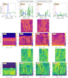 |
Fig. 4. Density profile (top) for longitudinally averaged (blue) and transverse profile at height y = 15 Mm (green) for each time. Time evolution of the density (middle) and velocity magnitude (bottom) for a case of θ = 88.5°. At time 85.9 s, the RT instability forms at the lower prominence-corona interface, corresponding to the early nonlinear phase. At time 257.6 s, the perturbed layer undergoes deformation due to the RT instability and forms bubbles and plumes as it transits to the later nonlinear phase. At time 515.2 s, the nonlinear phase further develops as part of the matter gets reflected upward, and we see the formation of further substructures on the edges of bubbles and plumes. At time 858.7 s, many small-scale structures in the prominence form, which transfer energy to intermediate scales, and turbulence is prominent at this time. |
The combination of an increased gas pressure against a decreasing magnetic pressure results in β increasing in time with the growing level of turbulence. As the simulation starts from an initial state of a quiescent prominence condition having a volume-averaged unit plasma β, the influence of magnetic pressure is important during the linear phase. As the nonlinear phase develops, the plasma β value increases throughout the transition of the system to a turbulent state, where the plasma pressure also affects the energy cascading processes through the formation of small-scale structures, as can be seen from Fig. 3. During the turbulent phase (see t = 858.7 s), the plasma β value increases considerably above the top of the initial prominence, where the plasma pressure becomes more dominant as compared to the magnetic pressure. The turbulence affects the detailed balance between kinetic, thermal, and magnetic energy. The local vertical profile of plasma beta at selected times is just one way of quantifying this transition. The buoyant rising of bubble-like structure seen in Fig. 4, in conjunction with the falling dense fingers, give instantaneous density variations at a height y= 15 Mm as shown in Fig. 4, top panels (green lines). These horizontal cuts show how density contrasts indeed remain strong between the pillars and plumes. Some matter is also entrained from the upper chromospheric regions on impacting the transition region, and then gets entrained up into our coronal volume. At late stages, the higher regions become beta unity and above, with buoyant matter rising through our top boundary and fine-scale mixing, causing the thermal pressure to rise. The various stages and the gradual trend to more and more fine-scale turbulence, especially after the falling pillars partially reflect off transition region heights and mix with upward and downward moving plasma, are particularly evident in the vorticity plots in Fig. 5.
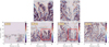 |
Fig. 5. Time evolution of the vorticity field for a case of θ = 88.5°. The initial stages show the onset of RT instability, followed by the formation of vortical structures in the shape of bubbles and plumes at 257.6 s. This then transitions to the late nonlinear phase at time 515.2 s, with the formation of small-scale structures due to the increasing shear at the edge of bubbles and plumes. At time 858.7 s, these substructures organize into vortices and other coherent structures, predominantly in the vertical direction. |
The magnetic field was initially set up to exert an upward magnetic pressure force to lift the prominence material locally. An evolving By(x, y) magnetic field component is established during the simulation. This is shown in Fig. 6, and one can note the development of many locations of nearby antiparallel poloidal (in-plane) field lines. This naturally plays a role in the (numerical) dissipative exchange of energy from magnetic to kinetic. After 257 s, one can even see shocks forming on top of the prominence. These shocks develop in the original, highly evacuated layer above the prominence, that is, where the derived initial density is very low and almost vacuum in nature. The shocks ultimately deform this top layer before it disappears through our open top boundary in the transient phase before about 500 s.
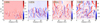 |
Fig. 6. Time evolution of By (magnetic field component in the stratified y direction) for a case of θ = 88.5°. Many locally antiparallel poloidal magnetic field lines are seen as the prominence flow transitions from a linear to a nonlinear phase. |
Figure 7 describes the density, temperature, and vorticity field of the truly turbulent state that is found at a later time. Indeed, the cool, dense material of the prominence collides with the transition region marking rapid changes in density and temperature, which leads to a significant rise of kinetic energy in the horizontal direction, as seen from Fig. 8A. After 800 s, we consider the prominence to transition to a fully turbulent state. In these nonlinear, turbulent stages, the full coronal region is to be considered as our prominence structure, which is now redistributed throughout the coronal domain. This is also seen in the way the x-averaged density profile above the transition region, as indicated in the blue lines in the top panels of Fig. 4, shows how most of the original prominence mass (from the integral under this curve) remains in the entire coronal region.
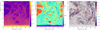 |
Fig. 7. Late time evolution of density, temperature, and vorticity field for a case of θ = 88.5° at time = 1073.38 s, when the prominence has dissipated. |
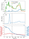 |
Fig. 8. Temporal evolution of physical quantities of the prominence. Panel A: Time evolution of the volume-averaged kinetic energy across the domain in the x and y directions and the volume-averaged total kinetic energy of the prominence. Panel B: Time evolution of the mean magnitude of the prominence’s vertical magnetic component, By (volume-averaged). Panel C: Evolution over time of the volume percentage of cool dense solar prominence (plus coronal interface) material, that is, excluding the chromosphere, taken below a threshold temperature of 5 × 10⁴ K, and denser than 10−11 kg m−3 (cf. Fig. 2), is plotted together with its corresponding mass. The dotted black line in Panel C represents the time 558.15 s, when the turbulence analysis was done. |
Figure 8A shows the evolution of the volume-averaged kinetic energy across the domain. The kinetic energy in the y direction increases during the transient period of shock development in the region above the initial prominence. Furthermore, the sharp increase of the magnetic field component in the y direction is also seen to succeed in this increase in kinetic energy according to Fig. 8B (see also Fig. 3). At these times, the falling material gets reflected back up from the sharp transition region gradients. Hence, the increase in the vertical kinetic energy describes the formation of the falling fingers and rising plumes associated with the linear and nonlinear phases of the RT instability. The rise in the height of the upper prominence boundary is mainly driven by the development of the bubbles, specifically. For the general RT instability, cool dense material gets accelerated in the downward direction in the presence of gravity. With time, the mixing of the plasma is then responsible for an increase in the volume of the cool dense material. In Fig. 8C, the time evolution of the percentage of the volume of cool material is plotted together with its mass. This is calculated by considering only the plasma below an upper threshold temperature of 5 × 10⁴ K and above a threshold density of 10−11 kg m−3. We can see that overall there is a slight decrease in the volume with a more significant decrease in the corresponding mass through the turbulent stages. This suggests that the degree of cool material that transits through the top boundary is partially compensated for by the mixing within the domain above the chromosphere boundary.
From Figs. 4 and 5 at time 515.2 s, we see the development of substructures along the edges of the large-scale bubbles and plumes, which are shown by the zoomed insets. Keppens et al. (2015) discussed the appearance of these small-scale structures in their simulation due to the strong shear flows established along the edges of the bubbles. These authors ran the simulation for only seven minutes in physical time and, as such, did not achieve the fully turbulent stages that we analyze in more detail here. These substructures lead to the formation of the KH instability and the vortices along the vertical direction, as seen from the velocity magnitude plots marked by the squares in Fig. 4. Mishra & Srivastava (2019) discussed evidence of magnetic RT-unstable plumes in a loop-like eruptive prominence. They suggested that the nonlinear phase of this magnetic RT-unstable plume collapses due to the formation of a KH vortex in the downfalling plasma. We observe the same process of downfalling prominence material accompanied by KH vortices in the nonlinear phase of our study.
In our study, the evolution of density structures shows turbulence developing in the prominence, indicated by the fine-scale structures present in Fig. 4. During time 858.7 s, the kinetic energy evolution from Fig. 8A, shows interesting behavior. The formation of small-scale structures in the horizontal (i.e., x) direction coincides with the increase in kinetic energy in the same direction. In the nonlinear stage, the cool and dense material, which is accelerated downward due to gravity, hits the evolving transition region and collects matter and energy from the chromosphere. This leads to an increase in fluctuations and build-up of kinetic energy in the horizontal direction. Until then, the kinetic energy was predominantly vertical, attributed to the linear and nonlinear stage development of the RT instability. Thus, the formation of vortices and swirling structures transfer energy among the scales and in both directions in this later stage. This turbulent stage is then analyzed in what follows.
3. Results for the turbulent stages
3.1. Observational counterparts
Quiescent prominences display a wide range of dynamics and structures predominantly oriented in the vertical direction (Berger et al. 2008). The vertical prominence structures are commonly characterized by dark upflows and the constant motion of streaming downflows, vortices, transverse oscillations, and expanding arch events. On the other hand, the horizontal prominence structure shows relatively little motion, with dynamics seemingly restricted to the appearance of short transient flows. The observational and theoretical work of Leonardis et al. (2012) implies that these features in quiescent prominence are together suggestive of turbulence. They applied statistical methods to the images from Hinode SOT Ca II H-Line observations to quantify the turbulent characteristics of a long-lived quiescent prominence. They investigated the multifractal and intermittent statistical scaling of turbulence properties for a long-lived quiescent prominence. Such turbulence in a finite region showed non-Gaussian statistics, multi-fractality, and extended self-similarity (ESS). These statistics gave information on scale behavior and correlation amongst scales and revealed non-Gaussianity through power-law distributions for the intensity fluctuations measured in time and space.
Similarly, Freed et al. (2016) used Ca II and Hα observations from Hinode to investigate the kinetic energy and vorticity associated with plasma flows in a quiescent prominence and found indices to the power-law fit to be in the range of −1 to −1.6. Hillier et al. (2017) used Hα Dopplergrams from Hinode SOT observations to investigate the turbulent nature of a prominence using SFs and showed the existence of two distinct regions with a break in the power law at around 2000 km. They also determined the non-Gaussianity and intermittent dynamics of the turbulence found within the observed prominence. The authors concluded that the heating rate due to turbulent dissipation is very small and unimportant in heating the prominence plasma. However, the diffusion due to magnetic reconnection is of a similar order to the estimated ambipolar diffusion and a few orders of magnitude greater than the Ohmic diffusion. These turbulent characteristics of plasma flow within solar prominences have so far primarily been addressed using observations. These studies focused on vertical and horizontal dynamics, where the former is characterized by extended, long-lived striations, and the latter form more short-lived, transient phenomena. The observational works analyze turbulence in terms of non-Gaussian statistics, multi-fractality, and ESS. In the following paragraphs, we go into more detail about each of these properties. The main aim of this work is to demonstrate that our simulated prominence exhibits properties in its turbulent stage that are very similar to the observed counterparts.
3.2. Analysis of the simulations
In order to understand the characteristics of the turbulence within our simulation, we process our MHD data and apply statistical methods. We use data at the full spatial resolution 1280 × 1280 at specific times. We also isolate a subset of the data spanning ∼25 min, with a cadence of ∼0.858 s, that covers the period of RT instability evolution within the prominence. Similar to the work of Leonardis et al. (2012), we use five strips each in the longitudinal and transverse directions, the former corresponding to the dominating vertical motion of flow in the prominence as seen in Fig. 9. For analysis, we consider the domain above the upper chromosphere boundary. Each longitudinal (transverse) strip has 1131 (1280) grid points along it, so a resolution of approximately 23 km. In practice, we take small ensembles consisting of 11 (five on either side of the center, inclusive) neighboring rows (columns) of grid cells for each strip in the transverse (longitudinal) direction. The statistical quantities are calculated for each of the 11 strips before averaging across this strip width to have more consistent statistics and capture the variation of any field in the spatial domain. Additionally, we use a single central point A within the domain, as shown in Fig. 9, to obtain the high-resolution time series of the temporal fluctuations within the simulation using the particle module of MPI-AMRVAC. We apply all our statistics to the fluctuating values of the field variables (velocity, magnetic components, or magnitude). We also apply statistics to the temperature field to enable a meaningful comparison to previous observational results. These fluctuating field variables are given by I′(u), which is obtained by subtracting the mean component from the instantaneous components of the fields, I′(u) = I(u)−⟨I(u)⟩, where u is either a spatial coordinate, x, or the temporal state, t, and the mean is  in the range u ∈ [umin, umax]. In what follows, we simplify the notation and hence write, for example, V(r)≡V′(r) for the fluctuation in the velocity field at location r instead.
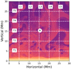 |
Fig. 9. Data divided into five longitudinal strips, L1-L5, and five transverse strips, T1–T5. The spatial analysis has been done for the fields at specific times. We also take time-sampled data at point A, where the temporal evolution of the data is stored at a cadence of 0.858 s (the density field of the solar prominence at time 858.7 s is shown in the background). |
For the spatial analysis, we analyze the two representative snapshots at time 558.15 s and 858.7 s in our simulation, where the structures in the transverse (i.e., x) direction start to grow compared to the longitudinal direction as seen in Fig. 8A, and we observe a turbulent state in our simulation. This can also be seen from the snapshots shown in Fig. 4, where the mixing has led to the formation of large-scale structures in both directions, deforming the clear bubble and plume shapes of the RT instability. In the statistical analysis, we take differences or increments at varying spatial and temporal separations (lags) denoted by L and τ, respectively. In Fig. 10, we show the instantaneous (strip-width averaged) spatial variation in the velocity field for the strip L5. In panel A we show the raw V(r), and its corresponding velocity increment of first differences δV = V(r + L)−V(r) in panel B, where r is the spatial coordinate (where r is either x or y for horizontal and/or vertical strips). For a spatial lag of L = 23 km along the strip, which hence subtracts the instantaneous neighbor value, panel B presents the spatial velocity series in the first difference δV(r, L = 1), which we find to be highly fluctuating with a consistent standard deviation across the mean. In an analogous fashion, the temporal series for sample point A in the setup, indicated in Fig. 9 from time 747.01 s to 1747.01 s, is shown in Fig. 10 (panels C and D) for the temporal variation of the velocity field, V(t), (panel C), and its corresponding time increment of first difference δV(t, τ) = V(t + τ)−V(t), (panel D), where t is the temporal scale and the temporal lag τ = 0.858 s.
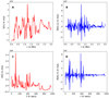 |
Fig. 10. Spatial series of the velocity field, V(r), for strip L5 (A) and the corresponding first difference, δV = V(r + L)−V(r), with L = 1 lag ∼23 km (B), for the prominence at time 858.7 s. The temporal series of the velocity field, V(t), from time 747.01 s to 1747.01 s, for point A in Fig. 9 is shown in (C). Its corresponding first difference, δV = V(t + τ)−V(t), with τ = 1 lag ∼0.858 s, is shown in (D). |
3.3. Correlation timescales
We analyzed the correlation time for the velocity and magnetic fields using the autocorrelation function normalized by the variance, that is, the correlation coefficient defined as
 (14)
(14)
where ⟨.⟩ denotes the average over the temporal direction t. This autocorrelation function is thus a function of the lag τ, which we vary in what follows in the range of 0.85 – 600 s for our analysis. The correlation coefficient value lies between −1 (perfectly anticorrelated), and +1 (perfectly correlated), while a zero value indicates uncorrelated data. Since turbulence is a random and stochastic phenomenon, the autocorrelation function converges to zero for the limit of a very large time lag, and one defines the correlation timescale, Tc, of the turbulence as
 (15)
(15)
Due to turbulence, the temporal correlation of the processes diminishes as the lag time τ increases. Due to this, the integral converges to give the correlation (or integral) timescale. The value of Tc gives the measure of memory of the turbulence (Pope 2000). In the case of a finite time sample series, one frequently uses an approximate T0, corresponding to the first zero crossing of the function R(τ = T0) = 0, to quantify this correlation time. From Fig. 11, we see that in our simulation data, we have a correlation time T0 of around 185 s for the velocity field and around 107 s for the magnetic field. A comparison can be made with Hillier et al. (2017) who found the correlation time for velocity to be 328 s. The intensity was 544 s, calculated using the half-width half-maximum (HWHM) of the auto-correlation.
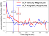 |
Fig. 11. Normalized temporal autocorrelation function (R(τ)) for the velocity and magnetic fields at the center of the simulation box (Point A in Fig. 9). The correlation time seen as the first zero crossing gives a correlation timescale of 185 s for the velocity field and a correlation timescale of 107 s for the magnetic field. |
In contrast to the observations, we can perform autocorrelation analysis for each vector component. All previous analysis of turbulence in prominences Leonardis et al. (2012), Freed et al. (2016), Hillier et al. (2017) was carried out on intensity images. In the present study, we make full use of the available field variables (magnetic field magnitude and plasma velocity field magnitude) and quantify their inter-dependence and influence on the turbulent characteristics of our simulation. The contribution of each vector component of the velocity and magnetic fields are shown in Figs. 12 (A and B), respectively. In the case of the velocity field, we see that the Vy has a longer correlation time, 246 s, compared to the Vx component at 178 s. The coherent structures remain for a longer time in the vertical direction and contribute to the increased growth of energy in this direction. This property has been previously observed within prominences (Engvold 1976). The velocity components become increasingly anticorrelated with time. The Bz component of the magnetic field is the largest component of the full magnetic field. Indeed, the correlation time for the Bz component is ten times longer (268 s) than for either the Bx (37 s) or By (21 s) components that are of a much smaller magnitude. This confirms how the anisotropic turbulence is influenced by the mean magnetic field orientation (the largest field component is Bz here, perpendicular to the simulation plane). The shorter correlation timescale for poloidal field components, and the longer one for the (mean) field component Bz, comparable to the poloidal velocity ones, is in accord with the anisotropy expected.
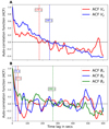 |
Fig. 12. Correlation timescales of individual velocity and magnetic field components. Panel A: Normalized temporal autocorrelation function for the x and y components of the velocity field at the center of the simulation box (Point A in Fig. 9). B: Normalized temporal autocorrelation function for the x, y, and z components of the magnetic field at the same location. Vy has the highest correlation timescale, 246 s, for the velocity components, compared to 178 s for Vx. Similarly, Bz has the highest correlation timescale, 268 s, compared to Bx with 37 s and By with 21 s. |
3.4. Power spectra
In the present study, the RT instability leads to the development of longitudinally (vertically) dominated structures in the shape of plumes and bubbles, which leads to the development of turbulence by forming initial large-scale disturbances or coherent structures in the solar atmosphere. At a later time, ∼500 s, the cool and dense material begins to collide with the upper chromosphere (transition region) boundary within our domain (the domain extends to lower chromospheric regions), leading to the rise of the structure’s transverse (horizontal) motions. This is indicated by the rise in the kinetic energy in the x direction in Fig. 8A around that time. An increasing amount of kinetic energy follows after 800 s in both x direction and y direction. Also, visually, this stage resembles a more fully turbulent flow. In a turbulent state, energy flows from the largest scales to the smallest or dissipative ones by a self-similar cascading process. In doing so, turbulence shows a power-law scaling in the power spectrum, namely, energy is transported at the same rate throughout the inertial range (Kolmogorov 1941).
We used the PSD to quantify energy distribution over spatial scales to estimate the power spectrum in a finite data set. If one applies the fast Fourier transform (FFT) method to a signal, one may be influenced by noise in the spectra at certain scales. The slope concerning those scales in this method might not have any physical meaning (Bruneau et al. 2005). To avoid this side effect, we calculated the PSD of the signal (spatial series) using the Welch periodogram method over the FFT using a Hanning window (Welch 1967). This periodogram helps in smoothing the sample sequence before computing the transform, segmenting the sample sequence, and computing additional estimators that can be averaged using overlapping sample sequences. We divided the transverse signal (I(r)) with 1280 points (the number of pixels along each strip) into G = 1280/M segments of M observations each (M < 1280), which are allowed to overlap (i.e., M is the size of each segment). If the segments do not overlap, a parameter S = M, while for a 50 % overlap, the parameter S = M/2. For each segment, we apply the Hanning window function and compute the windowed periodogram as
 (16)
(16)
where j = 1, …, G, and WS is the power of the window w(n) given by,  . The average of the windowed periodograms gives us the Welch PSD estimate,
 (17)
(17)
We followed the same procedure for the longitudinal signal with only 1131 points. Figure 13 shows log-log plots of PSDs for the (L3, L4) strips in the longitudinal and (T3, T4) strips in the transverse direction for the turbulence phase due to RT instability (top) and the fully turbulent phase (bottom). These two phases are defined by taking an ensemble average of snapshots taken before and after falling material collides with the chromosphere. The ensemble average for the first phase is taken between 558.15-772.83 s and 858.7-1073.38 s for the second phase. The velocity (Panel A and D), magnetic field (Panel B and E), and temperature field (Panel C and F) for the strips are shown in this figure for these two phases. We can see the energy cascades at similar rates for both phases in the field variables. The slope of linear fits to these log-log distributions provide us with the power-law scalings. For both phases, the error fits are calculated for the strips of a field along a direction between a common wavenumber range of 0.32 − 3.2 Mm−1 in all the panels.
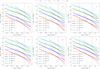 |
Fig. 13. PSD in the wavenumber domain for the longitudinal strips (L3, L4) and transverse strips (T3, T4) plotted for two ensemble averages of time before the collision of the material with the upper chromosphere boundary, representing a more RT instability turbulence (top), and after this collision led to more fully developed turbulence (bottom). All the PSDs are shifted on the y-axis for clarity. The dashed colored lines show fits of scalings done for a particular field in one direction between 0.32 and 3.2 Mm−1, as marked by the vertical dashed lines in all panels. There is a secondary steeper scaling of −3.5 at larger wavenumbers, as marked by the dotted black lines. |
From Fig. 13, we see that the power-law scaling values (also called the spectral index) for all the fields lies in the range between −1.84 and −2.6, and in Panel A of Fig. 13, the transverse velocity fluctuation is within one σ of the famous −5/3 spectra for isotropic, homogeneous hydrodynamic turbulence of Kolmogorov. The energy cascading processes on the larger scales in the inertial range is faster compared to such an ideal homogeneous turbulent flow. Of course, the presence of gravity and the perpendicular plane anisotropy likely plays a key role in our inhomogenous and stratified prominence setup, that is, the mixing and the energy dissipation process of the plasma is influenced by the in-plane magnetic field. The other fields also display scaling higher than Kolmogorov’s −5/3. We measured different scaling indices for the larger wavenumber ranges (> 3.2 Mm−1) when we did an estimated linear fit, though this gives the same average value around −3.5 at the end of the inertial range for all the strips (in both directions) for all the fields. The inertial range extends to the wavenumber, where the intermittency effect diminishes, and the unavoidable dissipation (numerical) effects take over in the smallest scales. The larger wavenumbers represent the dissipation scale, with the largest wavenumbers representing the scale of ∼23 km. Comparing the two phases for all the fields, we see shallow spectral indices as we move to more prevalent turbulent behavior throughout the prominence. This indicates that the turbulence level increases once the self-sustaining prominence dissipates as we depart from the RT instability. This behavior can be seen from Fig. 8A, where the rise of the horizontal kinetic energy in comparison to the vertical kinetic energy is observed. The coherent structures in the prominence that is initially dominated in the longitudinal direction are also seen to evolve in the transverse direction after the first phase.
As far as the observations were concerned, Leonardis et al. (2012) measured the PSDs for the intensity images and yielded slope values of −2 for the small wavenumbers ranges between 2.43 − 4.55 Mm−1 for the longitudinal strips and 2.07 − 4.61 Mm−1 for the transverse strips. At larger wavenumbers, their spectral index was around −3 for transverse strips and −2.7 for longitudinal strips. These values for the smaller wavenumbers are similar to that which we find for the velocity, magnetic, and temperature fields. In contrast, for larger wavenumber, our slope values are closer to −3.5. Such comparisons are most meaningful for the primitive temperature and velocity fields (and also, albeit to a lesser degree, for the magnetic field) as their structure and fluctuations influence to first order, albeit in a nontrivial manner, the emergent specific intensity recorded in observations.
3.5. Probability density functions
As is the case for many other physical systems, the turbulence within solar prominences is likely chaotic and disorganized, leading to entirely unpredictable plasma flows. A probabilistic description of turbulence of a field variable I at a position in space is given by its probability density function (PDF), P(I), where P(I)dI is the probability that the variable takes the value between I and I + dI such that it satisfies the normalization condition  .
.
For such an analysis, we must create a histogram of the signal, where all the possible signal values are binned into appropriately sized windows. Then the number of counts in each window is divided by the total number of realizations. We obtain the limiting curve of the PDF when the number of realizations increases without bounds as the size of the window goes to zero (George 2013). For this analysis, we concentrated on the turbulence due to the RT instability phase (i.e., at a time of around 558.15 s). For a stationary Gaussian process, the PDF behaves like a Gaussian, but in the presence of turbulence, the field deviates to a more non-Gaussian process with a heavy-tailed distribution. This is linked to the presence of intermittency or rare events in the signal, that is, large jumps in values outside of the standard deviation of the mean. This can be seen in the context of hydrodynamic turbulence (Anselmet et al. 1984; She et al. 1988; Castaing et al. 1990; Vincent & Meneguzzi 1991; Kailasnath et al. 1992; Mordant et al. 2001), in MHD turbulence (Müller & Biskamp 2000; Biskamp & Müller 2000; Homann et al. 2007; Biskamp 2003), and in solar wind turbulence (Burlaga 1993; Grauer et al. 1994; Politano & Pouquet 1995; Marsch & Tu 1997; Horbury & Balogh 1997; Sorriso-Valvo et al. 1999; Narita et al. 2006; Koga et al. 2007).
In Fig. 14 (panels A and B), the PDF of the velocity field increments δV(r, L) is plotted at fixed separations L of 0.468 Mm, 1.406 Mm, 2.344 Mm, 3.281 Mm, 4.219 Mm and 5.156 Mm in colored lines at time 558.15 s. This is done for the longitudinal L3 strip (A) and in a transverse T3 strip (B), where we normalize to the variance σ (i.e., P(δV) = δV/σ). For reference, the dashed black line is a Gaussian of unit variance plotted to show the degree of intermittency.
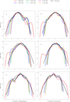 |
Fig. 14. PDF of the velocity (Panels A and B), magnetic (Panels C and D), and temperature field (Panels E and F) increments for L3 in the longitudinal (left) and T3 in the transverse direction (right) for increasing lags (or scales) of L = 0.468 Mm, 1.406 Mm, 2.344 Mm, 3.281 Mm, 4.219 Mm, and 5.156 Mm in the spatial domain plotted against the dashed black line of Gaussian distribution for the reference time 558.15 s. |
In Fig. 14 (panels C, D, E, and F), we plot the same for the magnetic field increments for L3 (C) and T3 strips (D) and temperature field increments for L3 (E) and T3 strips (F) using the same separations L, where we again normalize to the variance σ of the field. From these figures, we see that the distribution approaches Gaussianity at larger separations L. This can also be quantified by the fourth moment of the probability distribution, called Kurtosis, and given by the parameter K = ⟨P(δV)⟩4/σ4, which describes the extent of the peak in a distribution. Smaller values (in magnitude) indicate a flatter, more uniform probability distribution (George 2013). A Gaussian distribution is characterized by a Kurtosis value of 3 and  represents the coefficient of excess kurtosis defined as
  .
.
From Table 1, we see that the excess Kurtosis values for the PDF tend to decrease with increasing lag (separation scale) for the velocity, magnetic, and temperature fields. As such, the PDFs gradually become scale-independent with an increase in scale and eventually approach Gaussianity ( becomes close to zero). At such large scales, the fluctuations of the fields are therefore likely to be largely uncorrelated. The smaller scales, on the other hand, show a higher deviation from Gaussianity and indicate a higher rate of intermittent events happening at these scales. From Fig. 14, we see the presence of positively skewed values in the longitudinal velocity fields in the small scales describing upward vertical motions, whereas the longitudinal magnetic and temperature fields show more negative values describing downflows in the prominence. Frisch (1995) associates this behavior with intermittency; hence, our results show the existence of intermittency within prominence turbulence.

3.6. Structure functions
Turbulence within a solar prominence comprises fluctuations generated by the interaction of coherent structures of all varieties and sizes. Fully developed turbulence shows the property of scale invariance, which is characterized by a sequence of scaling exponents (Kolmogorov 1941; Frisch 1995). In the case of scale invariance, it is not possible to identify a predominant scale. Since the power spectrum is not enough for assessing scale invariance in the inertial range, it is necessary to look at higher-order moments. The PDFs qualitatively relate the turbulent dynamics found in prominences, which can be quantitatively realized by calculating the higher moments of these distributions. We use SFs, which are a measure of the correlation of fluctuations to length scales. An SF of order p of a field f(r) with lag L is defined by
 (18)
(18)
where we have taken the absolute value over the distribution and then carried out an ensemble average (we can, in practice, take the mean over the position range in r). The SF can describe the characteristics of the turbulent fluctuations in the inertial range, which exhibits a power-law function,
 (19)
(19)
where ζ(p) is the scaling exponent. When plotted logarithmically, ζ(p) gives the slope of the SF. A steeper slope would indicate more intermittency in the distribution. While if the slope changes with the scales, this indicates the change of intermittency as a function of the scale. This behavior is indeed seen in Fig. 15 for the velocity field (in A and B), the magnetic field (in C and D), and the temperature field (in E and F).
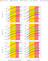 |
Fig. 15. SF (log-log) third order for longitudinal, L1–L5 (left), and transverse strips, T1–T5 (right), of the velocity field (A and B), magnetic field (C and D), and temperature field (E and F) at the reference time = 558.15 s. All the SFs are shifted on the y-axis for clarity. The rate of intermittency decreases with an increase in scales for A, B, C, D, E, and F. The yellow (α1) and light coral (α2) area mark the wavenumber between which the two error fits of power-law exponents are done for the scales of the individual strips. The values of these fits are given in Table 2. |
In the case of a self-similar assumption or a fractal (mono-fractal) process, which is a qualitative measure of having the same behavior of fluctuations at different scales, ζ(p) scales as a linear function of order p,
 (20)
(20)
where H is the Hurst exponent, ranging between 0 and 1, and Cp is a universal constant. In this case, the relation of the scaling exponent is simply ζ(p) = pH. However, fluid turbulence shows a deviation from the linearity of scaling exponents with higher orders of SFs, and this difference with the Kolmogorov self-similar law becomes higher with higher orders of p, indicating intermittency. The nonlinearity of the scaling exponent with p thus accounts for multifractal and intermittent behavior.
Figure 15 shows log-log plots of the third-order SF in the longitudinal direction (left) for L1–L5 strips and in the transverse direction for T1-T5 strips (right) for the velocity (A and B), magnetic (C and D), and temperature field (E and F) at time 558.15 s. The important point to note here is the presence of different slopes in the extended range of scales. We measured the power-law scaling values for the strips and calculated the error fits for the scales in two regions shown in Fig. 15 marked as vertical columns in yellow and light coral, respectively. The values of these indices for both strips are given in Table 2. In the smallest scales below 0.14 Mm, the scaling is steeper, implying that the intermittency is higher than in the larger scales. For the velocity (longitudinal and transverse) and temperature (longitudinal) fields, the second range of scales spans approximately between 0.14–0.96 Mm, as marked in the yellow (α1) column, where the slope value is higher in the longitudinal direction compared to the transverse direction. Beyond this range of scales, the third range spans between 0.96–6.3 Mm (marked as light coral α2 column), where the slope values decrease considerably compared to smaller scales for both directions. The third range in the transverse direction of the temperature field spans between 0.96–4.24 Mm. The scales in the range of 6.3 Mm may be the ones driving the upflows and downflows within prominences. The larger scales appear less correlated and may not be able to drive the mean flow arising from the RT instability. The increase of the SF with the scales implies a high correlation of the spatial fluctuations, resulting in the presence of coherent structures in the longitudinal direction.
In the transverse direction, similar to Leonardis et al. (2012) and Hillier et al. (2017), we find the presence of the knee within the range of 0.2–1.7 Mm for the velocity field and 1.4–5 Mm for temperature field approximately. Leonardis et al. (2012) found this knee range of scales to delimit the crossover between the small-scale turbulence and the large-scale coherent structures. This is also represented in Fig. 13, as the break in the power-law spectrum in the higher wavenumbers of the inertial range where energy is dissipated at a different rate between the small scales and larger scales. This knee could be attributed to an inverse cascade process (typical for true 2D MHD turbulence), which leads to a competition between the energy transfer scales and the intermittent scales responsible for energy dissipation.
As for the velocity and temperature field, Fig. 15 includes the SF of order 3 for the magnetic field in the longitudinal and transverse directions for each of the five strips. We find equivalent features in this case; however, the SFs in the longitudinal direction of the magnetic field are steeper and highly intermittent in the second range of scales (i.e., 0.14–0.96 Mm). As we move to higher scales in the magnetic field, the third range spans between 0.96–7.57 Mm in the longitudinal direction and 0.96–6.3 Mm in the transverse direction. The slope values for the third range of scales are lower than that of smaller scales for the magnetic fields, which we have already noted for the velocity and temperature fields. We also see the presence of the knee in the transverse direction of the magnetic field, lying approximately between 0.64–3.8 Mm.
Similar to Leonardis et al. (2012), we found that the SFs do not follow the power-law scaling given by Eq. (19), which describes a linear relationship of the scaling exponent ζ(p) with p. This may be attributed to systems limited by finite-range turbulence effects (Dubrulle 2000; Bershadskii 2007) where turbulence is not fully developed. As given by the theory of ESS (Benzi et al. 1993; Carbone et al. 1996), we can characterize the turbulence in the prominence using a set of scaling exponents ζ(p), by comparing SFs of a different order, p against q, which is given by
 (21)
(21)
We derive the ratio of the scaling exponents of different orders by calculating the slope of the line from the log-log plot of Sp versus Sq. We plot the same for S2 versus S3 in log-log scale to obtain the ratio of ζ(2)/ζ(3) from Fig. 16 for the velocity field (in A and B), magnetic field (in C and D), and temperature field (in E and F) at time 558.15 s; panels on the left (right) present the results for the five longitudinal (transverse) strips. Using linear regression fits for the curves over the whole range of scales in the inertial range, we obtain the values for the corresponding ratio of scaling exponents ζ(2)/ζ(3) for the longitudinal and transverse strips. The ratio ζ(2)/ζ(3) is shown for the corresponding direction and field in Table 3. They are found to be different from the linear value of 2/3 = 0.66 for each of the strips and imply the nonlinear form of the scaling exponents ζ(p). We thus find that the characteristics of turbulence in our simulated prominences due to the RT instability indicate multifractal behavior and show a high degree of intermittency in the smaller scales.
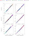 |
Fig. 16. ESS plots (log-log) of an SF of order 2 compared to an SF of order 3, for all longitudinal strips, L1–L5 (left), and transverse strips, T1–T5 (right), for the velocity field (A and B), magnetic field (C and D), and temperature field (E and F) at time = 558.15 s. A linear regression line fitting for the entire range of scales in the inertial range gives the slopes, or the scaling exponent ζ(2)/ζ(3) is shown in Table 3. The ζ(2)/ζ(3) values differ from the linear value of 0.66 in each of the cases, implying multi-fractality. |
We see from Fig. 15 that the small scales of the velocity, magnetic, and temperature fields are highly intermittent compared to the larger scales and, as such, with higher orders of SF (i.e., increasing p) would give more weight to extreme and rare events in a turbulent flow. Table 3 clearly gives the value of multi-fractality from ESS theory for order two compared to order three. In comparison, Fig. 17 shows the scaling exponents ζ(p)/ζ(3) for all the strips of the velocity (A and B), magnetic (C and D), and temperature (E and F) fields, against all orders from one to eight for longitudinal (transverse) in the left (right) panels for the two reference time. The black line shows the K41 (Kolmogorov 1941) self-similarity law, which behaves
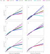 |
Fig. 17. Scaling exponent ζ(p)/ζ(3), inferred from the different slopes from Fig. 16 for the longitudinal (left) and transverse strips (right) for the velocity (A and B), magnetic (C and D), and temperature field (E and F) plotted versus order p, which goes from 1 to 8 at time 558.15 s. The dotted black line here represents the K41 self-similarity line or linear line (p/3). |
linearly with respect to the orders of SFs. For all the strips in the longitudinal and transverse direction of the velocity and the magnetic field, the scaling exponents deviate from the linear self-similarity line, and as such, the turbulence in prominence clearly shows intermittency behavior with a higher degree of nonlinearity as we focus on the smaller scales and increase the order of SFs. The exponents from higher-order SFs are prone to errors as with the increase on the order of p, it increasingly affects the Sp(L) in the presence of spurious large fluctuations. Leveque & She (1997) and Padoan et al. (2003) used a procedure to determine the highest significant order by calculating the peak of the histogram of |δf|p that occurs for a value of δf that must be represented by a significant number of points in the PDF of δf. Hillier et al. (2017) used an empirical way to calculate the highest order applicable with a reasonable noise for the study of higher-order SFs. So, we adopt caution on the exponent values for orders more than 6 in our case, as they might be susceptible to errors.
4. Conclusion
In this paper we use ideal MHD simulations in quiescent prominence conditions to analyze the turbulent characteristics obtained from the simulation data, which transitioned starting from a phase of the linear RT stage to nonlinear and, finally, to a turbulent stage at a much later time. The formation of coherent structures from falling bubbles and rising pillars into more organized structures predominantly in the vertical direction reveals the role of turbulence in mixing the stratified prominence flow. Earlier observations from Hinode SOT gave a first indication of the presence of turbulence within the prominences and the influence of characteristic scales on driving the turbulence. The analysis from observed intensity images was made under certain assumptions, such as that moving structures in the images follow the flow, acting as markers or passive scalars for the plasma dynamics. They were restricted to line-of-sight measurements. In our study, we have presented the results of an ideal MHD simulation representing a solar prominence within a 30 × 30 Mm domain. Once the dynamics within the simulation entered a turbulent state, analysis of these snapshots revealed and quantified the turbulent behavior of the magnetic and velocity field fluctuations.
We find a longer correlation time for the Vy component compared to the Vx component, indicating the vertical flows are more sustained, as remarked upon from observations. We investigated the power-law scaling that was evident from the PSDs of the velocity and the magnetic fields so as to ascertain the scaling at which energy was cascading from larger to smaller scales. We find these power-law scaling values to be steeper than the Kolmogorov’s k−5/3 scaling in the inertial range for the velocity, temperature, and magnetic fields. Additionally, there is a secondary scaling of k−3.5, identifiable for all the fields at the higher wavenumbers of the inertial range. This is suggestive of the turbulence within the simulation experiencing numerical dissipation in those wavenumbers. We observe shallow spectral indices for the fields as we move from the RT instability-generated prominence, which dissipates at a later time to a higher turbulent regime and represents higher turbulence behavior. As the fitting used to determine the spectral index is only performed over one decade, it can be very hard to relate the turbulent characteristics to the theoretical work of Kolmogorov or Iroshnikov-Kraichnan, so caution should be exercised. When we checked for intermittency, the PDFs of the velocity and magnetic field increments display a constant increase in spatial separations, indicating a departure from Gaussianity. The Kurtosis of the distributions further indicates the magnitude of the non-Gaussianity and intermittency. As we increase the separations, the distributions return to an approximate Gaussian, and the values of excess Kurtosis approach zero. At larger spatial scales, the distribution loses its coherency and becomes more Gaussian (i.e., the larger scales are less correlated). We note a more non-Gaussian distribution with higher intermittency for the smaller scales. We explore this further using SFs to analyze the behavior of these small scales within the inertial range and their role in developing turbulence across scales. The third-order SF illustrates different slope values for the scales in the inertial range, which can be classified into three ranges. The steeper the slope, the higher the degree of intermittency present. The first range, the smallest scales, up to 0.14 Mm for all the fields, is steeper in the longitudinal direction compared to the transverse direction, which is the same for the second range of scales, between 0.14–0.96 Mm, for the velocity, temperature, and magnetic fields in both directions. Similar to observations (Leonardis et al. 2012; Freed et al. 2016; Hillier et al. 2017), we note a break in the SFs across the scales of around 2–5 Mm for the velocity, magnetic, and temperature fields in the transverse direction, which was previously interpreted as a physical limit in the ability of small-scale turbulence to cross over into the larger scales. The longitudinal velocity increments also show a higher degree of correlation, constituting the domination of flow in the vertical direction, which is also seen in observations. Finally, the degree of multifractal turbulence is shown with the ratio of scaling exponents ζ(2)/ζ(3), whose values differ from the self-similar assumption of linearity or fractal turbulence (i.e., 0.66).
In the present numerical study of prominence formation due to RT instability, we studied the development of prominence features within a 2.5D setup with the mean magnetic field directed into the plane. We used an ideal MHD prescription, and hence the scales where numerical dissipation matters will be strongly sensitive to the chosen numerical resolution. We plan to address true dissipation effects in follow-up work, where we will use fully converged, resistive MHD studies at numerically affordable (i.e., below actual) magnetic Reynolds numbers. There are limitations with the current choice of 2.5D setup, and it might not be an accurate representation of the 3D turbulence that can develop in the solar prominence, but our numerical simulation presents a strong case that RT instability is one of the main contributors to turbulence in prominences. In our 2.5D setup, plasma flow is heavily influenced by the out-of-plane mean-magnetic field, so we urgently need a fully 3D counterpart for this study. We note that the chosen initial angle of the magnetic field to the simulated poloidal plane influences the linear instability properties and the ensuing turbulence. In our setup, magnetic tension is initially zero, since the 2.5D setup has only magnetic pressure support for the prominence. Magnetic tension in the simulated plane does play a role within the further evolutions, as shown in Fig. 6. But, of course, future 3D work can start from more realistic, magnetic-tension-supported prominence models where the dense matter initially rests in upwardly concave dips.
Furthermore, in an ideal MHD setup, we do not consider the dissipative scales, which have an effect on both the linear and nonlinear phase of the ensuing numerical magnetic reconnection within the simulation. Magnetic reconnection is responsible for the intermittent events of heating and energy dissipation. Hillier & Polito (2021), using observations from the Interface Region Imaging Spectrograph (IRIS), investigated the occurrence of magnetic reconnection events through the ejection of bi-directional blobs along the current sheet developed within an observed prominence. We will look at such reconnection events in a numerical resistive model follow-up study under prominence conditions. The magnetic Prandtl number is given by Pm = Rm/Re = ν/η, where Rm is the magnetic Reynolds number, Re is the Reynolds number, ν is the kinematic viscosity, and η is the magnetic diffusivity. This parameter determines which scale is larger: the viscous dissipation scale or the resistive dissipation scale. In the solar atmosphere, the value is very low. Thus, in order to conclude more about the effects of these scales, we need to include the resistive MHD model within our simulation setup. Moreover, our model lacks additional system physics, such as the Hall effect, partial ionization (ambipolar diffusion), different ion-electron temperatures, radiative losses, and thermal conduction. The inclusion of any combination of these effects would extend our understanding of turbulence within solar prominences. This will be the focus of future endeavors.
Movie
Movie 1 associated with Fig. 3 (density_RTI) Access Supplementary Material
Acknowledgments
This work was supported by the ERC Advanced Grant PROMINENT, and an FWO grant G0B4521N. This project has received funding from the European Research Council (ERC) under the European Union’s Horizon 2020 research and innovation programme (grant agreement No. 833251 PROMINENT ERC-ADG 2018). This research is further supported by Internal funds KU Leuven, through the project C14/19/089 TRACESpace.
References
- Anselmet, F., Gagne, Y., Hopfinger, E. J., & Antonia, R. A. 1984, J. Fluid Mech., 140, 63 [NASA ADS] [CrossRef] [Google Scholar]
- Arber, T. D., Haynes, M., & Leake, J. E. 2007, ApJ, 666, 541 [Google Scholar]
- Benzi, R., Ciliberto, S., Tripiccione, R., et al. 1993, Phys. Rev. E, 48, R29 [CrossRef] [Google Scholar]
- Berger, T. E., Shine, R. A., Slater, G. L., et al. 2008, ApJ, 676, L89 [Google Scholar]
- Berger, T. E., Slater, G., Hurlburt, N., et al. 2010, ApJ, 716, 1288 [Google Scholar]
- Berger, T. E., Testa, P., Hillier, A., et al. 2011, Nature, 472, 197 [NASA ADS] [CrossRef] [Google Scholar]
- Bershadskii, A. 2007, J. Stat. Phys., 128, 721 [NASA ADS] [CrossRef] [Google Scholar]
- Biskamp, D. 2003, Magnetohydrodynamic Turbulence [Google Scholar]
- Biskamp, D., & Müller, W.-C. 2000, Phys. Plasmas, 7, 4889 [NASA ADS] [CrossRef] [Google Scholar]
- Bommier, V., & Leroy, J. L. 1998, ASP Conf. Ser., 150, 434 [NASA ADS] [Google Scholar]
- Bruneau, C. H., Fischer, P., Peter, Z., & Yger, A. 2005, Sampling Theory in Signal and Image Processing, 4, 169 [CrossRef] [Google Scholar]
- Burlaga, L. F. 1993, J. Geophys. Res. Space Phys., 98, 17467 [NASA ADS] [CrossRef] [Google Scholar]
- Carbone, V., Veltri, P., & Bruno, R. 1996, Nonlinear Proc. Geophys., 3, 247 [NASA ADS] [CrossRef] [Google Scholar]
- Casini, R., López Ariste, A., Tomczyk, S., & Lites, B. W. 2003, ApJ, 598, L67 [Google Scholar]
- Castaing, B., Gagne, Y., & Hopfinger, E. J. 1990, Phys. D Nonlinear Phenom., 46, 177 [NASA ADS] [CrossRef] [Google Scholar]
- Chae, J. 2010, ApJ, 714, 618 [NASA ADS] [CrossRef] [Google Scholar]
- Chandrasekhar, S. 1961, Hydrodynamic and Hydromagnetic Stability (Oxford, UK: Oxford Univ. Press) [Google Scholar]
- Collados, M., Trujillo Bueno, J., & Asensio Ramos, A. 2003, ASP Conf. Ser., 307, 468 [NASA ADS] [Google Scholar]
- Dedner, A., Kemm, F., Kröner, D., et al. 2002, J. Comput. Phys., 175, 645 [Google Scholar]
- Díaz, A. J., Soler, R., & Ballester, J. L. 2012, ApJ, 754, 41 [Google Scholar]
- Díaz, A. J., Khomenko, E., & Collados, M. 2014, A&A, 564, A97 [NASA ADS] [CrossRef] [EDP Sciences] [Google Scholar]
- Dubrulle, B. 2000, Eur. Phys. J. B, 14, 757 [NASA ADS] [CrossRef] [Google Scholar]
- Engvold, O. 1976, Sol. Phys., 49, 283 [NASA ADS] [CrossRef] [Google Scholar]
- Engvold, O. 1981, Sol. Phys., 70, 315 [NASA ADS] [CrossRef] [Google Scholar]
- Freed, M. S., McKenzie, D. E., Longcope, D. W., & Wilburn, M. 2016, ApJ, 818, 57 [Google Scholar]
- Frisch, U. 1995, Turbulence. The legacy of A.N. Kolmogorov (Cambridge: Cambridge University Press) [CrossRef] [Google Scholar]
- George, W. K. 2013, Lectures in Turbulence for the 21st Century (Chalmers University of Technology) [Google Scholar]
- Gibson, S. E. 2018, Liv. Rev. Sol. Phys., 15, 7 [Google Scholar]
- Goedbloed, H., Keppens, R., & Poedts, S. 2019, Magnetohydrodynamics: Of Laboratory and Astrophysical Plasmas (Cambridge University Press) [Google Scholar]
- Grauer, R., Krug, J., & Marliani, C. 1994, Phys. Lett. A, 195, 335 [NASA ADS] [CrossRef] [Google Scholar]
- Hillier, A. 2018, Rev. Mod. Plasma Phys., 2, 1 [Google Scholar]
- Hillier, A., & Polito, V. 2021, A&A, 651, A60 [NASA ADS] [CrossRef] [EDP Sciences] [Google Scholar]
- Hillier, A., Isobe, H., Shibata, K., & Berger, T. 2011, ApJ, 736, L1 [Google Scholar]
- Hillier, A., Berger, T., Isobe, H., & Shibata, K. 2012a, ApJ, 746, 120 [Google Scholar]
- Hillier, A., Isobe, H., Shibata, K., & Berger, T. 2012b, ApJ, 756, 110 [Google Scholar]
- Hillier, A., Matsumoto, T., & Ichimoto, K. 2017, A&A, 597, A111 [NASA ADS] [CrossRef] [EDP Sciences] [Google Scholar]
- Hirayama, T. 1986, NASA Conf. Publ., 2442, 149 [NASA ADS] [Google Scholar]
- Homann, H., Grauer, R., Busse, A., & Müller, W. C. 2007, J. Plasma Phys., 73, 821 [NASA ADS] [CrossRef] [Google Scholar]
- Horbury, T. S., & Balogh, A. 1997, Nonlinear Proc. Geophys., 4, 185 [NASA ADS] [CrossRef] [Google Scholar]
- Innes, D. E., Cameron, R. H., Fletcher, L., Inhester, B., & Solanki, S. K. 2012, A&A, 540, L10 [NASA ADS] [CrossRef] [EDP Sciences] [Google Scholar]
- Jenkins, J. M., & Keppens, R. 2022, Nat. Astron., 6, 942 [NASA ADS] [CrossRef] [Google Scholar]
- Kailasnath, P., Sreenivasan, K. R., & Stolovitzky, G. 1992, Phys. Rev. Lett., 68, 2766 [Google Scholar]
- Kaneko, T., & Yokoyama, T. 2018, ApJ, 869, 136 [Google Scholar]
- Keppens, R., & Xia, C. 2014, ApJ, 789, 22 [Google Scholar]
- Keppens, R., Meliani, Z., van Marle, A., et al. 2012, J. Comput. Phys., 231, 718 [Google Scholar]
- Keppens, R., Xia, C., & Porth, O. 2015, ApJ, 806, L13 [Google Scholar]
- Keppens, R., Teunissen, J., Xia, C., & Porth, O. 2021, Comput. Math. Appl., 81, 316 [Google Scholar]
- Khomenko, E., Díaz, A., de Vicente, A., Collados, M., & Luna, M. 2014, A&A, 565, A45 [NASA ADS] [CrossRef] [EDP Sciences] [Google Scholar]
- Kippenhahn, R., & Schlüter, A. 1957, Z. Astrophys., 43, 36 [Google Scholar]
- Koga, D., Chian, A. C. L., Miranda, R. A., & Rempel, E. L. 2007, Phys. Rev. E, 75, 046401 [NASA ADS] [CrossRef] [Google Scholar]
- Kolmogorov, A. 1941, Akademiia Nauk SSSR Doklady, 30, 301 [Google Scholar]
- Koren, B. 1993, A Robust Upwind Discretization Method for Advection, Diffusionand Source Terms, Afdeling Numerieke Wiskunde: Report NM (Centrum voor Wiskunde en Informatica) [Google Scholar]
- Kubota, J., & Uesugi, A. 1986, PASJ, 38, 903 [NASA ADS] [Google Scholar]
- Leonardis, E., Chapman, S. C., & Foullon, C. 2012, ApJ, 745, 185 [Google Scholar]
- Levens, P. J., Schmieder, B., López Ariste, A., et al. 2016, ApJ, 826, 164 [NASA ADS] [CrossRef] [Google Scholar]
- Leveque, E., & She, Z.-S. 1997, Phys. Rev. E, 55, 2789 [NASA ADS] [CrossRef] [Google Scholar]
- Liggett, M., & Zirin, H. 1984, Sol. Phys., 91, 259 [NASA ADS] [CrossRef] [Google Scholar]
- Luna, M., Karpen, J., Ballester, J. L., et al. 2018, ApJS, 236, 35 [NASA ADS] [CrossRef] [Google Scholar]
- Mackay, D., Karpen, J., Ballester, J., Schmieder, B., & Aulanier, G. 2010, Space Sci. Rev., 151, 333 [NASA ADS] [CrossRef] [Google Scholar]
- Marsch, E., & Tu, C. Y. 1997, Nonlinear Proc. Geophys., 4, 101 [NASA ADS] [CrossRef] [Google Scholar]
- Martínez-Sykora, J., De Pontieu, B., Hansteen, V., & Carlsson, M. 2015, Philos. Trans. R. Soc. London Ser. A, 373, 20140268 [Google Scholar]
- Merenda, L., Trujillo Bueno, J., Landi Degl’Innocenti, E., & Collados, M. 2006, ApJ, 642, 554 [Google Scholar]
- Mishra, S. K., & Srivastava, A. K. 2019, ApJ, 874, 57 [NASA ADS] [CrossRef] [Google Scholar]
- Miyoshi, T., & Kusano, K. 2005, J. Comput. Phys., 208, 315 [NASA ADS] [CrossRef] [Google Scholar]
- Mordant, N., Metz, P., Michel, O., & Pinton, J. F. 2001, Phys. Rev. Lett., 87, 214501 [Google Scholar]
- Müller, W.-C., & Biskamp, D. 2000, Phys. Rev. Lett., 84, 475 [CrossRef] [Google Scholar]
- Narita, Y., Glassmeier, K. H., & Treumann, R. A. 2006, Phys. Rev. Lett., 97, 191101 [Google Scholar]
- Padoan, P., Boldyrev, S., Langer, W., & Nordlund, Å. 2003, ApJ, 583, 308 [NASA ADS] [CrossRef] [Google Scholar]
- Politano, H., & Pouquet, A. 1995, Phys. Rev. E, 52, 636 [NASA ADS] [CrossRef] [Google Scholar]
- Pope, S. B. 2000, in Turbulent Flows (Cambridge, UK: Cambridge University Press), 806 [Google Scholar]
- Popescu Braileanu, B., Lukin, V. S., Khomenko, E., & de Vicente, Á. 2021a, A&A, 646, A93 [NASA ADS] [CrossRef] [EDP Sciences] [Google Scholar]
- Popescu Braileanu, B., Lukin, V. S., Khomenko, E., & de Vicente, A. 2021b, A&A, 650, A181 [NASA ADS] [CrossRef] [EDP Sciences] [Google Scholar]
- Popescu Braileanu, B., Lukin, V. S., & Khomenko, E. 2021c, A&A, 670, A31 [Google Scholar]
- Porth, O., Xia, C., Hendrix, T., Moschou, S. P., & Keppens, R. 2014, ApJS, 214, 4 [Google Scholar]
- Priest, E. R. 1982, Geophys. Astrophys. Monogr., 21, 19 [NASA ADS] [Google Scholar]
- Ruderman, M. S., Terradas, J., & Ballester, J. L. 2014, ApJ, 785, 110 [Google Scholar]
- Rust, D. M. 1967, ApJ, 150, 313 [NASA ADS] [CrossRef] [Google Scholar]
- Ruuth, S. J., & Spiteri, R. J. 2002, J. Sci. Comput., 17, 211 [CrossRef] [Google Scholar]
- Ryutova, M., Berger, T., Frank, Z., Tarbell, T., & Title, A. 2010, Sol. Phys., 267, 75 [Google Scholar]
- Schwartz, P., Gunár, S., Jenkins, J. M., et al. 2019, A&A, 631, A146 [NASA ADS] [CrossRef] [EDP Sciences] [Google Scholar]
- She, Z.-S., Jackson, E., & Orszag, S. A. 1988, J. Sci. Comput., 3, 407 [NASA ADS] [CrossRef] [Google Scholar]
- Sorriso-Valvo, L., Carbone, V., Veltri, P., Consolini, G., & Bruno, R. 1999, Geophys. Res. Lett., 26, 1801 [NASA ADS] [CrossRef] [Google Scholar]
- Tandberg-Hanssen, E. 1995, The Nature of Solar Prominences (Dordrecht: Kluwer Academic Publishers), 199 [Google Scholar]
- Terradas, J., Soler, R., Luna, M., Oliver, R., & Ballester, J. L. 2015, ApJ, 799, 94 [Google Scholar]
- Terradas, J., Soler, R., Luna, M., et al. 2016, ApJ, 820, 125 [Google Scholar]
- Vincent, A., & Meneguzzi, M. 1991, J. Fluid Mech., 225, 1 [NASA ADS] [CrossRef] [Google Scholar]
- Welch, P. D. 1967, IEEE Trans. Audio Electroacoust, 15, 70 [CrossRef] [Google Scholar]
- Xia, C., & Keppens, R. 2016a, ApJ, 823, 22 [Google Scholar]
- Xia, C., & Keppens, R. 2016b, ApJ, 825, L29 [NASA ADS] [CrossRef] [Google Scholar]
- Xia, C., Teunissen, J., El Mellah, I., Chané, E., & Keppens, R. 2018, ApJS, 234, 30 [Google Scholar]
- Zhou, Y., Williams, R. J. R., Ramaprabhu, P., et al. 2021, Phys. D Nonlinear Phenom., 423, 132838 [NASA ADS] [CrossRef] [Google Scholar]
All Tables
All Figures
|
Fig. 1. Number of grids per AMR level during the evolution of the flow. |
| In the text | |
|
Fig. 2. Derived density (top) and enforced initial temperature (bottom) profiles in the vertical direction at the initial state. The temperature is set to be 8000 K in the chromosphere and transitions to 1.8 × 10⁶ K for the corona, dropping at y = yb to 6000 K for the lower part of the prominence. It then has a linear increasing profile from 6000–14 000 K at y = yp to y = 20 Mm for the upper part of the prominence. |
| In the text | |
|
Fig. 3. Local plasma beta (averaged in the x direction) in the initial prominence of the reference case θ = 88.5° at t = 0 s (red) compared to its evolution in time at t= 85.9 s, 257.6 s, 515.2 s, and 858.7 s. |
| In the text | |
|
Fig. 4. Density profile (top) for longitudinally averaged (blue) and transverse profile at height y = 15 Mm (green) for each time. Time evolution of the density (middle) and velocity magnitude (bottom) for a case of θ = 88.5°. At time 85.9 s, the RT instability forms at the lower prominence-corona interface, corresponding to the early nonlinear phase. At time 257.6 s, the perturbed layer undergoes deformation due to the RT instability and forms bubbles and plumes as it transits to the later nonlinear phase. At time 515.2 s, the nonlinear phase further develops as part of the matter gets reflected upward, and we see the formation of further substructures on the edges of bubbles and plumes. At time 858.7 s, many small-scale structures in the prominence form, which transfer energy to intermediate scales, and turbulence is prominent at this time. |
| In the text | |
|
Fig. 5. Time evolution of the vorticity field for a case of θ = 88.5°. The initial stages show the onset of RT instability, followed by the formation of vortical structures in the shape of bubbles and plumes at 257.6 s. This then transitions to the late nonlinear phase at time 515.2 s, with the formation of small-scale structures due to the increasing shear at the edge of bubbles and plumes. At time 858.7 s, these substructures organize into vortices and other coherent structures, predominantly in the vertical direction. |
| In the text | |
|
Fig. 6. Time evolution of By (magnetic field component in the stratified y direction) for a case of θ = 88.5°. Many locally antiparallel poloidal magnetic field lines are seen as the prominence flow transitions from a linear to a nonlinear phase. |
| In the text | |
|
Fig. 7. Late time evolution of density, temperature, and vorticity field for a case of θ = 88.5° at time = 1073.38 s, when the prominence has dissipated. |
| In the text | |
|
Fig. 8. Temporal evolution of physical quantities of the prominence. Panel A: Time evolution of the volume-averaged kinetic energy across the domain in the x and y directions and the volume-averaged total kinetic energy of the prominence. Panel B: Time evolution of the mean magnitude of the prominence’s vertical magnetic component, By (volume-averaged). Panel C: Evolution over time of the volume percentage of cool dense solar prominence (plus coronal interface) material, that is, excluding the chromosphere, taken below a threshold temperature of 5 × 10⁴ K, and denser than 10−11 kg m−3 (cf. Fig. 2), is plotted together with its corresponding mass. The dotted black line in Panel C represents the time 558.15 s, when the turbulence analysis was done. |
| In the text | |
|
Fig. 9. Data divided into five longitudinal strips, L1-L5, and five transverse strips, T1–T5. The spatial analysis has been done for the fields at specific times. We also take time-sampled data at point A, where the temporal evolution of the data is stored at a cadence of 0.858 s (the density field of the solar prominence at time 858.7 s is shown in the background). |
| In the text | |
|
Fig. 10. Spatial series of the velocity field, V(r), for strip L5 (A) and the corresponding first difference, δV = V(r + L)−V(r), with L = 1 lag ∼23 km (B), for the prominence at time 858.7 s. The temporal series of the velocity field, V(t), from time 747.01 s to 1747.01 s, for point A in Fig. 9 is shown in (C). Its corresponding first difference, δV = V(t + τ)−V(t), with τ = 1 lag ∼0.858 s, is shown in (D). |
| In the text | |
|
Fig. 11. Normalized temporal autocorrelation function (R(τ)) for the velocity and magnetic fields at the center of the simulation box (Point A in Fig. 9). The correlation time seen as the first zero crossing gives a correlation timescale of 185 s for the velocity field and a correlation timescale of 107 s for the magnetic field. |
| In the text | |
|
Fig. 12. Correlation timescales of individual velocity and magnetic field components. Panel A: Normalized temporal autocorrelation function for the x and y components of the velocity field at the center of the simulation box (Point A in Fig. 9). B: Normalized temporal autocorrelation function for the x, y, and z components of the magnetic field at the same location. Vy has the highest correlation timescale, 246 s, for the velocity components, compared to 178 s for Vx. Similarly, Bz has the highest correlation timescale, 268 s, compared to Bx with 37 s and By with 21 s. |
| In the text | |
|
Fig. 13. PSD in the wavenumber domain for the longitudinal strips (L3, L4) and transverse strips (T3, T4) plotted for two ensemble averages of time before the collision of the material with the upper chromosphere boundary, representing a more RT instability turbulence (top), and after this collision led to more fully developed turbulence (bottom). All the PSDs are shifted on the y-axis for clarity. The dashed colored lines show fits of scalings done for a particular field in one direction between 0.32 and 3.2 Mm−1, as marked by the vertical dashed lines in all panels. There is a secondary steeper scaling of −3.5 at larger wavenumbers, as marked by the dotted black lines. |
| In the text | |
|
Fig. 14. PDF of the velocity (Panels A and B), magnetic (Panels C and D), and temperature field (Panels E and F) increments for L3 in the longitudinal (left) and T3 in the transverse direction (right) for increasing lags (or scales) of L = 0.468 Mm, 1.406 Mm, 2.344 Mm, 3.281 Mm, 4.219 Mm, and 5.156 Mm in the spatial domain plotted against the dashed black line of Gaussian distribution for the reference time 558.15 s. |
| In the text | |
|
Fig. 15. SF (log-log) third order for longitudinal, L1–L5 (left), and transverse strips, T1–T5 (right), of the velocity field (A and B), magnetic field (C and D), and temperature field (E and F) at the reference time = 558.15 s. All the SFs are shifted on the y-axis for clarity. The rate of intermittency decreases with an increase in scales for A, B, C, D, E, and F. The yellow (α1) and light coral (α2) area mark the wavenumber between which the two error fits of power-law exponents are done for the scales of the individual strips. The values of these fits are given in Table 2. |
| In the text | |
|
Fig. 16. ESS plots (log-log) of an SF of order 2 compared to an SF of order 3, for all longitudinal strips, L1–L5 (left), and transverse strips, T1–T5 (right), for the velocity field (A and B), magnetic field (C and D), and temperature field (E and F) at time = 558.15 s. A linear regression line fitting for the entire range of scales in the inertial range gives the slopes, or the scaling exponent ζ(2)/ζ(3) is shown in Table 3. The ζ(2)/ζ(3) values differ from the linear value of 0.66 in each of the cases, implying multi-fractality. |
| In the text | |
|
Fig. 17. Scaling exponent ζ(p)/ζ(3), inferred from the different slopes from Fig. 16 for the longitudinal (left) and transverse strips (right) for the velocity (A and B), magnetic (C and D), and temperature field (E and F) plotted versus order p, which goes from 1 to 8 at time 558.15 s. The dotted black line here represents the K41 self-similarity line or linear line (p/3). |
| In the text | |
Current usage metrics show cumulative count of Article Views (full-text article views including HTML views, PDF and ePub downloads, according to the available data) and Abstracts Views on Vision4Press platform.
Data correspond to usage on the plateform after 2015. The current usage metrics is available 48-96 hours after online publication and is updated daily on week days.
Initial download of the metrics may take a while.