| Issue |
A&A
Volume 691, November 2024
|
|
|---|---|---|
| Article Number | A84 | |
| Number of page(s) | 20 | |
| Section | Interstellar and circumstellar matter | |
| DOI | https://doi.org/10.1051/0004-6361/202450338 | |
| Published online | 31 October 2024 | |
Impact of H I cooling and study of accretion disks in asymptotic giant branch wind-companion smoothed particle hydrodynamic simulations
1
Institute of Astronomy, KU Leuven,
Celestijnenlaan 200D,
3001
Leuven,
Belgium
2
Institut d’Astronomie et d’Astrophysique, Université Libre de Bruxelles (ULB),
CP 226,
1050
Brussels,
Belgium
3
University of Amsterdam, Anton Pannekoek Institute for Astronomy,
Amsterdam,
1098
XH,
The Netherlands
★ Corresponding author; This email address is being protected from spambots. You need JavaScript enabled to view it.
Received:
12
April
2024
Accepted:
20
August
2024
Abstract
Context. High-resolution observations reveal that the outflows of evolved low- and intermediate-mass stars harbour complex morphological structures that are linked to the presence of one or multiple companions. Hydrodynamical simulations provide a way to study the impact of a companion on the shaping of the asymptotic giant branch (AGB) star out-flow.
Aims. Using smoothed particle hydrodynamic (SPH) simulations of an AGB star undergoing mass loss, which also has a binary companion, we study the impact of including H I atomic line cooling on the flow morphology. We also study how this affects the properties of the accretion disks that form around the companion.
Methods. We used the PHANTOM code to perform high-resolution 3D SPH simulations of the interaction of a solar-mass companion with the outflow of an AGB star, using different wind velocities and eccentricities. We compared the model properties, computed with and without the inclusion of H I cooling.
Results. The inclusion of H I cooling produces a sizeable decrease in the temperature, up to one order of magnitude, in the region closely surrounding the companion star. As a consequence, the morphological irregularities and relatively energetic (bipolar) outflows that were obtained without H I cooling no longer appear. In the case of an eccentric orbit and a low wind velocity, these morphologies are still highly asymmetric, but the same structures recur at every orbital period, making the morphology more regular. Flared accretion disks, with a (sub-)Keplerian velocity profile, are found to form around the companion in all our models with H I cooling, provided the accretion radius is small enough. The disks have radial sizes ranging from about 0.4 to 0.9 au and masses around 10−7−10−8 M⊙. For the considered wind velocities, mass accretion onto the companion is up to a factor of 2 higher than predicted by the standard Bondi Hoyle Littleton rate, ranging between ~4 to 21% of the AGB wind mass loss rate. The lower the wind velocity at the location of the companion, the larger and the more massive the disk and the higher the mass accretion efficiency. In eccentric systems, the disk size, disk mass, and mass accretion efficiency vary, depending on the orbital phase.
Conclusions. H I cooling is an essential ingredient to properly model the medium around the companion where density-enhanced wind structures form and it favours the formation of an accretion disk.
Key words: methods: numerical / stars: AGB and post-AGB / binaries: general / stars: winds, outflows
© The Authors 2024
 Open Access article, published by EDP Sciences, under the terms of the Creative Commons Attribution License (https://creativecommons.org/licenses/by/4.0), which permits unrestricted use, distribution, and reproduction in any medium, provided the original work is properly cited.
This article is published in open access under the Subscribe to Open model. This email address is being protected from spambots. You need JavaScript enabled to view it. to support open access publication.
1 Introduction
When low- and intermediate-mass stars reach the asymptotic giant branch (AGB) evolutionary phase, they shed their outer layers through a strong, pulsation-enhanced, dust-driven stellar wind, with mass-loss rates of ![Mathematical equation: $\[\dot{M}\]$](/articles/aa/full_html/2024/11/aa50338-24/aa50338-24-eq1.png) ~ 10−8−10−5 M⊙ yr−1 (Höfner & Olofsson 2018; Decin 2021). These out-flows span a large range in density and temperature, making them interesting chemical laboratories that contribute to ~85% of the gas and ~35% of the dust enrichment of the inter-stellar medium (ISM; Tielens 2005). For decades, these outflows were believed to be spherically symmetric and they were modelled in a one-dimensional (1D) approach. However, high-resolution observations reveal that asymmetrical structures such as spirals, arcs, disks, and bipolar outflows are embedded in the winds of AGB stars (Mauron & Huggins 2006; Maercker et al. 2012; Decin et al. 2020; Danilovich et al. 2024). The environment of post-AGB stars and planetary nebulae (PNe), that descend from these AGB circumstellar envelopes (CSEs), are also known to show complex morphologies, including: bipolar nebulae and shells (Balick & Frank 2002) and consecutive rings and arcs (Ramos-Larios et al. 2016). Currently, the main theories for the formation of non-spherical planetary nebulae involve interactions with one or more companions (De Marco 2009; De Marco et al. 2013; Jones & Boffin 2017; Akashi & Soker 2017; García-Segura et al. 2018). Likewise, the complex morphologies of post-AGB stars are linked to the presence of a binary system with a circumbinary disk and to a companion with circumstellar accretion disk and bipolar jets; however, the exact formation mechanism is unknown (Van Winckel 2003; Bollen et al. 2022; Corporaal et al. 2023; Verhamme et al. 2024; De Prins et al. 2024). These post-AGB binaries are often found in highly eccentric orbits with periods of 102−104 days (Oomen et al. 2018; Jorissen et al. 2019; Escorza et al. 2019). This is in strong disagreement with population synthesis results, which predict closer, circularised orbits due to tides, or wider, possibly eccentric orbits (Toonen et al. 2012). Similarly, it is now commonly believed that the observed structures in AGB outflows are the result of the impact of companions that are hidden within the dense wind. This hypothesis is supported by binary population statistics (Moe & Di Stefano 2017; Offner et al. 2023), which states that about 50% of solar mass stars has a binary companion, with this percentage increasing with stellar mass. Further, several recent observational studies of AGB stars manage to identify the indirect presence of a companion, for example, through its impact on molecular abundances (Ramstedt et al. 2014; Kervella et al. 2016; Homan et al. 2020; Decin et al. 2020; Danilovich et al. 2024; Planquart et al. 2024). Finally, high-resolution 3D hydrodynamic simulations of binary AGB stars reveal how complex structures naturally emerge from the presence of a companion. The earliest studies of this type (Theuns & Jorissen 1993; Theuns et al. 1996; Mastrodemos & Morris 1998, 1999) had already shown that Archimedes-like spiral structures, elongated morphologies, and accretion disks can form naturally, depending on the orbital and wind parameters of the modelled system. Later higher resolution simulations analysed in more detail the formation of different structures, including spirals, arc- and ring-shaped morphologies, equatorial density enhancements, and accretion disks. These works studied the impact of these structures on the mass transfer and orbital evolution (see e.g. Kim & Taam 2012; Kim et al. 2019; Chen et al. 2017, 2020; Liu et al. 2017; Saladino et al. 2018, 2019; El Mellah et al. 2020; Malfait et al. 2021; Maes et al. 2021; Aydi & Mohamed 2022). The structures that arise in the AGB wind due to binary interaction, might play an important role in the shaping of the CSE at later evolutionary stages. For example, Lora et al. (2023) use 3D radiation-hydrodynamic models to mimic the transition from the AGB to the proto-PN phase by artificially ejecting jets and a spherically symmetric fast wind, after a spiral structure has already been shaped in the AGB wind by a companion star. With this method, they have been able to recover the morphologies of proto-PNe and PNe with ring-like structures in their haloes.
~ 10−8−10−5 M⊙ yr−1 (Höfner & Olofsson 2018; Decin 2021). These out-flows span a large range in density and temperature, making them interesting chemical laboratories that contribute to ~85% of the gas and ~35% of the dust enrichment of the inter-stellar medium (ISM; Tielens 2005). For decades, these outflows were believed to be spherically symmetric and they were modelled in a one-dimensional (1D) approach. However, high-resolution observations reveal that asymmetrical structures such as spirals, arcs, disks, and bipolar outflows are embedded in the winds of AGB stars (Mauron & Huggins 2006; Maercker et al. 2012; Decin et al. 2020; Danilovich et al. 2024). The environment of post-AGB stars and planetary nebulae (PNe), that descend from these AGB circumstellar envelopes (CSEs), are also known to show complex morphologies, including: bipolar nebulae and shells (Balick & Frank 2002) and consecutive rings and arcs (Ramos-Larios et al. 2016). Currently, the main theories for the formation of non-spherical planetary nebulae involve interactions with one or more companions (De Marco 2009; De Marco et al. 2013; Jones & Boffin 2017; Akashi & Soker 2017; García-Segura et al. 2018). Likewise, the complex morphologies of post-AGB stars are linked to the presence of a binary system with a circumbinary disk and to a companion with circumstellar accretion disk and bipolar jets; however, the exact formation mechanism is unknown (Van Winckel 2003; Bollen et al. 2022; Corporaal et al. 2023; Verhamme et al. 2024; De Prins et al. 2024). These post-AGB binaries are often found in highly eccentric orbits with periods of 102−104 days (Oomen et al. 2018; Jorissen et al. 2019; Escorza et al. 2019). This is in strong disagreement with population synthesis results, which predict closer, circularised orbits due to tides, or wider, possibly eccentric orbits (Toonen et al. 2012). Similarly, it is now commonly believed that the observed structures in AGB outflows are the result of the impact of companions that are hidden within the dense wind. This hypothesis is supported by binary population statistics (Moe & Di Stefano 2017; Offner et al. 2023), which states that about 50% of solar mass stars has a binary companion, with this percentage increasing with stellar mass. Further, several recent observational studies of AGB stars manage to identify the indirect presence of a companion, for example, through its impact on molecular abundances (Ramstedt et al. 2014; Kervella et al. 2016; Homan et al. 2020; Decin et al. 2020; Danilovich et al. 2024; Planquart et al. 2024). Finally, high-resolution 3D hydrodynamic simulations of binary AGB stars reveal how complex structures naturally emerge from the presence of a companion. The earliest studies of this type (Theuns & Jorissen 1993; Theuns et al. 1996; Mastrodemos & Morris 1998, 1999) had already shown that Archimedes-like spiral structures, elongated morphologies, and accretion disks can form naturally, depending on the orbital and wind parameters of the modelled system. Later higher resolution simulations analysed in more detail the formation of different structures, including spirals, arc- and ring-shaped morphologies, equatorial density enhancements, and accretion disks. These works studied the impact of these structures on the mass transfer and orbital evolution (see e.g. Kim & Taam 2012; Kim et al. 2019; Chen et al. 2017, 2020; Liu et al. 2017; Saladino et al. 2018, 2019; El Mellah et al. 2020; Malfait et al. 2021; Maes et al. 2021; Aydi & Mohamed 2022). The structures that arise in the AGB wind due to binary interaction, might play an important role in the shaping of the CSE at later evolutionary stages. For example, Lora et al. (2023) use 3D radiation-hydrodynamic models to mimic the transition from the AGB to the proto-PN phase by artificially ejecting jets and a spherically symmetric fast wind, after a spiral structure has already been shaped in the AGB wind by a companion star. With this method, they have been able to recover the morphologies of proto-PNe and PNe with ring-like structures in their haloes.
In previous work by Malfait et al. (2021) (henceforth, Paper I), 3D smoothed particle hydrodynamic (SPH) simulations where performed with the PHANTOM code1 (Price et al. 2018), for a grid of nine AGB binary-wind models, with different orbital eccentricities and wind velocities. Their main conclusions were as follows. For high wind velocities (initial velocity υini = 20 km s−1), the limited gravitational attraction of the companion on the wind particles results in a two-edged spiral structure originating behind the companion. This stable wind structure shapes the global morphology into a regular Archimedes spiral in the orbital plane, with concentric arcs in the meridional plane. For lower wind velocities, more wind material is compressed around the companion into a high-pressure bubble, which is delimited by a bow shock spiral originating in front of the companion. In case of an intermediate wind velocity (υini = 10 km s−1), this high-pressure region and bow shock are stable, resulting in a regular spiral with meridional bicentric rings. When the wind velocity is very low (υini = 5 km s−1), periodic instabilities occur around the high-pressure region, in some cases followed by relatively energetic outflows with radial velocities up to 30 km s−1. This results in irregular morphologies in both the orbital and meridional plane view. In case the orbit is eccentric, the phase-dependency of the wind-companion interaction strength introduces additional complexities. The wind structures close to the stars vary throughout the orbital phases and instabilities are more likely to occur, potentially resulting in highly asymmetric wind morphologies. The instabilities that occurred were associated with hot wind material with gas temperatures reaching T ≥ 105 K that accumulated around the companion.
In this work, we include H I atomic line cooling in our SPH model, following Spitzer (1978) (see Sect. 2). This cooling has been considered in previous simulations by Mastrodemos & Morris (1998, 1999) and Chen et al. (2017) to provide an efficient cooling especially impacting the material in the close vicinity of the companion. We selected six of the simulations analysed in Paper I and studied the effect of H I cooling on the wind structures (Sect. 3). Due to the presence of cooling, accretion disks form around the solar-mass companion. We perform higher-resolution simulations focusing on these accretion disks, and study in detail their morphology and properties, how they change for different input wind velocities and in eccentric orbits, and how efficiently mass is accreted through the disks (Sect. 4). Our conclusions are presented in Sect. 6.
2 Method
2.1 Input physics
The hydrodynamic simulations are performed with the smoothed particle hydrodynamics (SPH) code PHANTOM (Price et al. 2018). The numerical set-up of our models is the same as the one described in Paper I and Maes et al. (2021), but with additional cooling in the form of H I atomic line cooling. The wind consists of SPH gas particles, that follow the adiabatic equation of state (EOS):
![Mathematical equation: $\[P=(\gamma-1) \rho u,\]$](/articles/aa/full_html/2024/11/aa50338-24/aa50338-24-eq2.png) (1)
(1)
where P is the pressure, ρ the gas density, u the internal energy, and γ the polytropic index. The gas temperature T is obtained using Eq. (1) and the ideal gas law:
![Mathematical equation: $\[P=\frac{\rho k_{\mathrm{B}} T}{\mu m_{\mathrm{H}}},\]$](/articles/aa/full_html/2024/11/aa50338-24/aa50338-24-eq3.png) (2)
(2)
where kB is Boltzmann’s constant, mH the mass of a hydrogen atom, and μ is the mean molecular weight. The polytropic index γ and mean molecular weight μ are set to a constant value throughout the model, with γ = 1.2 a typical value to account for the temperature profile in AGB winds (Millar 2004; Maes et al. 2021), and μ = 2.38 or 1.26 depending on whether we consider a molecular or atomic wind, respectively (see also Table 1). We note, however, that the temperature profile is not imposed throughout the simulations, and greatly depends on the cooling and heating mechanisms.
In this work, H I cooling is included in the set-up through an implicit integration method that is acting on substeps. The cooling term is calculated by use of the relation
![Mathematical equation: $\[\Lambda_{\text {cool_HI }}=7.3 \times 10^{-19} \mathrm{~g} \mathrm{~cm}^3 \times \frac{n_e n_{\mathrm{H}} \mathrm{e}^{-118~400 \mathrm{~K} / T}}{\rho} \mathrm{erg} \mathrm{~g}^{-1} \mathrm{~s}^{-1},\]$](/articles/aa/full_html/2024/11/aa50338-24/aa50338-24-eq4.png) (3)
(3)
presented in Spitzer (1978), where ne and nH are the electron and total hydrogen number density, respectively (for details see Appendix D). This cooling is mostly effective at the high temperatures reached inside shocks or close to an accreting companion, and becomes dominant at temperatures above ~8000 K (Bowen 1988). This term is included in the energy equation, along with adiabatic work done by expansion and compression, and shock heating Λshock (Price et al. 2018), as
![Mathematical equation: $\[\frac{\mathrm{d} u}{\mathrm{~d} t}=-\frac{P}{\rho}(\boldsymbol{\nabla} \cdot \boldsymbol{\nu})+\Lambda_{\text {shock }}-\Lambda_{\text {cool_HI }}.\]$](/articles/aa/full_html/2024/11/aa50338-24/aa50338-24-eq5.png) (4)
(4)
The binary companion is modelled by a sink particle, with an accretion radius Rs,accr, such that gas particles and their mass and momentum are indiscriminately accreted by the companion sink particle if they fall within 0.8 Rs,accr; additional checks on gravitational binding and angular momentum were performed in the boundary region 0.8 Rs,accr < r < Rs,accr, as described in Sect. 2.8.2 of Price et al. (2018). To model the wind, SPH particles are distributed on spheres around the primary sink particle and assigned an initial velocity υini (for details, see Siess et al. 2022; Esseldeurs et al. 2023). To drive the wind, the free-wind approximation is used, in which the gravity of the AGB star is artificially balanced by the radiation force (introduced by Theuns & Jorissen 1993). Although this approximation does not take into account the complex driving mechanism of dust-driven winds, it avoids additional assumptions on e.g. pulsations, dust, and luminosity, while still retrieving reasonable results in the low mass-loss rate regime (Esseldeurs et al. 2023).
Initial binary model set-up.
2.2 Simulation grid set-up
We calculated a grid of six models to analyse how H I cooling impacts the wind-companion interaction and resulting wind morphologies. The set-up parameters are presented in Table 1. As in Paper I, the primary star is an AGB star with a mass of Mp = 1.5 M⊙, accretion radius of Rp,accr = 1.2 au = 258 R⊙, and effective temperature of Tp = 3000 K. The AGB star is part of a binary system with a solar-mass companion of Ms = 1 M⊙, located at a semi-major axis of a = 6 au; this gives the binary an orbital period of Porb = 9.3 yr and orbital velocities of υorb,p, = 7.69 km s−1 and υorb,c = 11.54 km s−1. The stars are deep in their potential well, with Roche radii of 2.487 au and 2.066 au for the primary and secondary, respectively.
The simulations were run for 10 orbital periods, corresponding to tmax = 93 yr. The grid of binary models is presented in Table 2, and is a selection of the models analysed in Paper I, but with H I cooling included. To study the effect of orbital eccentricity, we model systems with eccentricities e = 0 and e = 0.5. Furthermore, we considered systems with input wind velocities of υini = 5, 10 and 20 km s−1 to model different wind-companion interaction regimes and wind morphologies (El Mellah et al. 2020; Malfait et al. 2021; Maes et al. 2021). The mass-loss rate of the AGB star was set to ![Mathematical equation: $\[\dot{M}\]$](/articles/aa/full_html/2024/11/aa50338-24/aa50338-24-eq8.png) = 10−7 M⊙ yr−1. For wind velocities of ~20 km s−1 observations (Ramstedt et al. 2020) suggested higher mass-loss rates, but by setting the same
= 10−7 M⊙ yr−1. For wind velocities of ~20 km s−1 observations (Ramstedt et al. 2020) suggested higher mass-loss rates, but by setting the same ![Mathematical equation: $\[\dot{M}\]$](/articles/aa/full_html/2024/11/aa50338-24/aa50338-24-eq9.png) for all simulations, we isolate the effect of changing the wind velocity, without introducing an additional variable parameter (we come back to this in Sect. 5.3). Moreover, we note that a better treatment of radiative acceleration (not assuming a free-wind) is needed to optimally model the effect of the mass-loss rate on the resulting wind structures (Esseldeurs et al. 2023).
for all simulations, we isolate the effect of changing the wind velocity, without introducing an additional variable parameter (we come back to this in Sect. 5.3). Moreover, we note that a better treatment of radiative acceleration (not assuming a free-wind) is needed to optimally model the effect of the mass-loss rate on the resulting wind structures (Esseldeurs et al. 2023).
Compared to Paper I, we slightly increased the boundary radius, that sets the distance from the AGB sink particle above which particles are removed from the simulation, from 200 to 250 au. We also slightly decreased the accretion radius of the companion, Rs,accr = 0.05 au, to Rs,accr = 0.04 au = 8.6 R⊙. By decreasing Rs,accr, we increased the computation time, but we enhanced our ability to numerically resolve an accretion disk around the companion. At the end of the computation, the simulations have reached a quasi-steady state and contain ~106 particles. We note that the precise number depends on the input wind velocity and the number of particles that are accreted and thereby removed from the simulation.
Binary model characteristics.
3 Impact of H I cooling on binary simulations
In Paper I, cooling was regulated by the EOS of an ideal gas with a polytropic index γ = 12, without additional cooling mechanisms. This led to the formation of a high-pressure region around the companion star, where the SPH particles reached temperatures above 105 K in combination with high velocities. This gave rise to periodic instabilities and energetic outflows both in the direction of the orbital plane and towards the poles. Here, we include a cooling mechanism that reduces the temperatures in this hot region around the companion and study the effect on the wind shaping.
The main effects of including H I atomic line cooling are as follows. First, the disappearance of periodic instabilities that occurred due to heated-up material around the companion, and that were giving rise for example to a square-like structure in model v05e00 of Paper I. Second, the material around the companion is instead cooled down by about an order of magnitude; it is able to accumulate and form an accretion disk, which we study in detail in Sect. 4 with higher resolution models. Third, the bipolar outflows with velocities up to ~30 km s−1 that developed in the low AGB wind velocities simulations described in Paper I are no longer present in our improved models. Fourth, even with H I cooling and formation of stable accretion disks, complex, very asymmetric wind morphologies emerge in the eccentric systems. Finally, cooling also decreases the wind velocity in the enhanced density wind structures, which affects the outflow morphology. These effects are discussed in more detail below. Following the same format as Paper I, we analyse the wind structures that are created close to the stars, and the larger-scale wind morphologies that result from them. Although the addition of H I cooling yields a more realistic temperature distribution, in most of our simulations, the resulting temperatures in the inner wind region are still too high for efficient dust nucleation to take place. Therefore, additional cooling mechanisms, such as molecular or atomic fine structure line cooling, are required to model a self-consistent dust-driven wind.
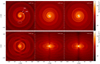 |
Fig. 1 Density profile in a slice through (top row) and perpendicular to (bottom row) the orbital plane of binary models v20e00 (left), v10e00 (middle), and v05e00 (right) at the end of the simulation (t = 93 yr), with log = (log10). The AGB and companion star are marked as the left and right dot, respectively, not to scale. In the upper left panel, the ‘backward spiral edge’ (BSE), the ‘frontward spiral edge’ (FSE), and the location where they merge into one spiral structure are indicated. A version without H I cooling is presented in Fig. 1 in Paper I. |
3.1 Wind structures in circular binary systems, with H I cooling
For the three non-eccentric systems v05e00, v10e00, and v20e00 (with initial wind velocities of υini = 5, 10, and 20 km s−1) the density distribution in the orbital and meridional plane is shown in the top and bottom row in Fig. 1, respectively. The same plots for the models without cooling are presented in Fig. 1 in Paper I. In models v20e00 (left column) and v10e00 (middle column), the global wind structures presented in these figures appear not significantly altered by the inclusion of H I cooling. In the low wind velocity model v05e00 (left column), however, the wind morphology is strongly impacted by the H I cooling.
3.1.1 Model v20e00
In model v20e00 (Fig. 1, left column), the passage of the companion in the AGB wind creates a spiral structure in the wake behind the companion, best seen in the orbital plane. The gravitational slingshot effect creates a velocity dispersion leading to the formation of a radially slower inner ‘backward spiral edge’ (BSE) and faster moving outward ‘frontward spiral edge’ (FSE). For a more detailed description, we refer to Paper I and Maes et al. (2021). After an orbital period of ~1.25, the FSE merges with the BSE that originated one orbital period earlier (indicated at x ≈ 0, y ≈ −50 au in the upper left panel of Fig. 1) and one Archimedean spiral structure results. The spirals can be approximated by a mathematical Archimedean spiral described by Eqs. (6)-(9) in Paper I, with the approximate radial velocity of the wind particles within the two spiral edges of υr,BSE = 11 km s−1 and υr,FSE = 19.5 km s−1. Figure 2 shows the orbital plane velocity distribution (left) and the analytical Archimedean spiral (right) for comparison. This figure illustrates once again how the faster FSE catches up with the slower BSE around x = 0 au, y = −50 au. Following this interaction, the FSE dominates the global orbital plane spiral structure.
One difference seen with respect to model v20e00 in Paper I without H I cooling is the much lower (radial) velocity of the FSE and of the material within the two-edged gravity wake behind the companion, which results in a smaller opening angle of the two-edged wake. This can be seen in Fig. A.12 that compares the pressure, temperature, internal energy, and velocity distribution in the inner wind region of the model with (top row) and without (bottom row) H I cooling. Figure A.1 reveals that with H I cooling the internal energy, u, and temperature, T, of the wind particles decrease within the wake, which in turn lowers the pressure, P, (Eq. (1)) and velocity, v. More precisely, the temperature closely around the companion drops by an order of magnitude from ~105 to ~104 K. Further away from the companion, after an orbital phase of π/2 (around x = 0, y < 0 in Fig. A.1) the temperature within the gravity wake has decreased from ~3 × 10⁴ to ~104 K. This cooling by a factor of ~3 remains present further out in the wind, up to large radii, as can be seen in Fig. A.22. As a result, the radial velocity of the FSE (υr,FSE = 19.5 km s−1) is about ~4.5 km s−1 lower than the approximated velocity in Paper I (υr,FSE,paperI = 24 km s−1). The consequences of this slower FSE are the following. At first, because the velocity of the BSE has not decreased, the width of the gravity wake, so the radial distance between the BSE and FSE, is smaller. Secondly, the FSE catches up with the BSE later, and in this model about half an orbital period later. At last, the inter-arm distance between two windings of the resulting Archimedean spiral is shorter, as this distance is determined by the radial distance the spiral material travels during one orbital period. In the meridional plane (Fig. 1, bottom left), the 3D spiral of model v20e00 is displayed in the form of concentric arcs. The same three effects of the lower radial velocity of the material within the spiral as described for the orbital plane spiral can be identified. The banana-shaped arcs are again delineated by the BSE and FSE (respectively the edge closest to and furthest away from the stars). Due to the inclusion of H I cooling (i) the width of the arcs is smaller, (ii) the FSE catches up with a previous BSE later, and (iii) the inter-arc distance after overlap is smaller, making the entire morphology appear more compressed.
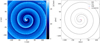 |
Fig. 2 Velocity profile in a slice through the orbital plane (left) and analytical Archimedean spiral fit of the merging ‘backward spiral edge’ (BSE) and ‘frontward spiral edge’ (FSE) of model v20e00 (right). A version without H I cooling is presented in Figs. 2 and 3 of Paper I. |
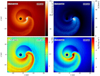 |
Fig. 3 Density, velocity, temperature, and pressure profile in the orbital plane of model v10e00, superimposed with the velocity vector profile which is shown as black arrows. A version without H I cooling is presented in Fig. 4 of Paper I. |
3.1.2 Model v10e00
In models v10e00 and v05e00 (middle and right column of Fig. 1), the gravitational impact of the companion on the wind material is stronger due to the lower wind velocity, so that more material can accumulate around the companion. Similarly to model v20e00, an Archimedean spiral structure results in the orbital plane, but the wind structure close to the companion differs.
Figure 3 displays the density, velocity, temperature and pressure distribution in the orbital plane close to the stars of model v10e00. Instead of one two-edged spiral, there is one dense inner flow behind the companion that wraps tightly around the AGB star, and that terminates as it collides with a bow shock spiral (around x ≈ 9 au, y ≈ 1 au) that originates in front of the moving companion. As can be seen in the density plot in Fig. 1 (middle column, top row), the bow shock spiral itself is delineated again by a slower BSE and faster FSE, and after almost one orbit the FSE catches up with the previous BSE (around x = 35 au, y = 20 au in these plots) such that one Archimedean spiral results (for a more detailed description, see Sect. 3.1.2 in Paper I).
The density and pressure distribution in Fig. 3 show the dense inner spiral flow behind the companion, and the less dense bow shock spiral (and can be compared to Fig. 4 in Paper I without H I cooling). The first, main impact of the cooling is in the material closely surrounding the companion (around x = 3.6 au, y = 0 au). In this region, the gas temperature has dropped by more than an order of magnitude from T ≳ 105 K to T ≲ 104 K, such that the bow shock particles also have significantly lower temperatures. As a result of this decreased temperature, more wind material can accumulate closely around the companion, and is gravitationally captured into an accretion disk. The high density results in a high pressure, such that this circumstellar disk is also clearly visible in the pressure distribution plot (see Sect. 4). A second difference caused by the cooling is that, analogously to model v20e00, the decrease in internal energy results in a lower pressure, and thereby a lower radial velocity of the material within the high-density Archimedean spiral and FSE. This makes the orbital plane inter-arm and meridional plane inter-arc distance smaller, such that the global morphology is more compressed (which can be seen from comparison of the middle row in Fig. 1 and Fig. 1 in Paper I).
3.1.3 model v05e00
Without H I cooling, the low AGB wind velocity in model v05e00 resulted in an unstable region around the companion. This led to irregular wind structures with a square orbital plane spiral and irregular meridional morphology (presented in Sect. 3.1.3. in Paper I). With H I cooling, the morphology of model v05e00 (shown on the right column of Fig. 1) is very similar to the one of model v10e00, with a regular Archimedean spiral in the orbital plane, and regular bicentric arcs in the meridional plane.
Figure A.32 confirms that the density, velocity, temperature and pressure distribution in the orbital plane close to the stars is almost the same as for model v10e00 (Fig. 3). Figure A.42 shows the density and temperature distribution around the companion at two different time-steps within one orbital period. Because the material around the companion is now efficiently cooled down to T ≲ 104 K, the previous instabilities with irregular varying wind structures (visible in Fig. 5 of Paper I) no longer appear. Instead, there is a stable bow shock and accretion disk (studied in more detail in Sect. 4).
3.2 Eccentric models
In cases where the binaries are in eccentric orbits, the wind-companion interaction becomes phase-dependent. Thus, the companion spends more time around apastron passage, while the gravitational interaction with the wind is stronger when it resides in the higher density region near the shorter periastron passage. In the circular orbit models, the wind structure created close to the companion (such as the two-edged spiral or bow shock) does not change. The phase-dependency in the eccentric models implies that the type of structure around the stars varies throughout one orbital period. These varying inner structures then travel radially outward with the wind, making the global morphology asymmetric.
Figure 4 shows the density distribution of the binary models with eccentricity e = 0.5 (top row: v20e05, middle row: v10e50, bottom row: v05e50) in three different perpendicular slices (left: orbital plane xy, middle: edge-on xz, right: edge-on yz). This figure illustrates the asymmetry, diversity and irregularity in three dimensions of the AGB outflow of eccentric binaries. Compared to the same models without cooling (which can be found in Paper I in Fig. 6 (v20e50, right column), Fig. 10 (v10e50, second row), and Fig. 13 (v05e50, third row), the current density morphologies harbour similar features and are slightly more regular, but still asymmetric, as we explain in the following paragraphs in more detail.
3.2.1 v20e50
Apart from overall asymmetry, two other features characteristic of eccentric systems are low-density gaps and bifurcations (Kim et al. 2019; Malfait et al. 2021). Bifurcations are locations where two spirals seem to split up or come together, and they arise at the edges of the low-density regions. These features appear in model v20e50, as can be seen in Fig. 4, where the darker-coloured low-density gaps are marked by white arrows, and the bifurcations are encircled. These characteristic patterns are created through the phase-dependent wind-companion interaction, which makes the inner wind structure vary between a two-edged spiral and bow shock, as is explained in detail in Sect. 3.2.1. of Paper I. The same mechanism is shaping the wind in model v20e50, with the main difference that because of the cooling, the companion is surrounded by an accretion disk throughout all orbital phases, as discussed in more detail in Sect. 4. Figure A.52 displays the density, velocity, temperature and pressure distribution close to the stars at four consecutive orbital phases. In the top row, the stars just passed periastron passage, and the companion is surrounded by an accretion disk and a bow shock. This is similar to the simulation without H I cooling (presented in Fig. 9 of Paper I), except that now there is an accretion disk instead of a ‘high-energy’ bubble, so the radial extent of the bow shock surrounding this region is now also much smaller. Towards the apastron passage (second row), the increase of orbital separation induces a decrease in the orbital velocity of the companion. The radially outward moving bow shock tends to overtake the companion, which results in a larger opening angle, more towards the front of the companion. After the apastron passage (third row) the companion orbits radially inward again with an increasing orbital velocity. This creates a kink in the structure behind the companion, as can be seen in time steps 2 and 3 of Fig. A.52. The decreasing wind-companion interaction around apastron induces again the creation of a two-edged spiral structure without bow shock (third and fourth row). The companion keeps its accretion disk, which remains present throughout every orbital phase (see Fig. 17 in Sect. 4).
3.2.2 v10e50 and v05e50
The characteristic low-density gaps and bifurcations do not form in the models with lower wind velocity. Because of the stronger wind-companion interaction intensity, the eccentricity causes asymmetric wind structures that deviate stronger from the regular spiral-arc morphology of non-eccentric binaries. These morphologies are displayed in the density distribution in the middle and bottom row of Fig. 4, for models v10e50 and v05e50, respectively. Contrary to the simulations without cooling (displayed in Figs. 10 and 13 of Paper I), the wind morphology is much more regular, and self-similar (recurrent density structures at different radii, originating at specific orbital phases). Additionally, the simulations without H I cooling harboured bipolar outflows, which are now no longer present, as can be seen in the edge-on velocity plots in Fig. A.62.
Figures 5 and 6 display the density and temperature distribution in the orbital plane slice close to the stars at two different orbital phases. Because of the low wind velocity and the eccentric nature of the orbit, the wind structures around the companion do not only strongly vary because of the phase-dependent wind-companion interaction, but they also interact and collide with other high density structures that originated one orbital period earlier and were very tightly wound around the AGB star. The inclusion of cooling prevents the formation of hot, escaping ‘high-energy’ bubbles after apastron passage, which were described in Paper I (in Figs. 12 and 14). However, there are similarities in the shaping of the wind structures. For example, when the star is orbiting from periastron to apastron passage (e.g. at t = 80.74 yr), there is always a bow shock, but in the model with cooling, the opening angle is smaller. For a better visualisation of how these structures vary over each orbital period, and how the bow shock interacts with other high density structures, we refer to online movie 1 (see Appendix E) showing the evolution of the density distribution in the orbital plane slice of system v10e50 in Fig. 5 in a co-rotating coordinate frame. The temperature plots in Figs. 5 and 6 confirm that the H I cooling is efficient in the region closely around the companion sink particle, which used to have temperatures T > 105 K (as shown in Figs. 11 and 14 in Paper I).
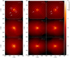 |
Fig. 4 Density distribution in a slice through the orbital plane (left, x-y plane) and in two perpendicular meridional plane slices (middle, x-z plane, and right, y-z plane) of the three eccentric binary models v20e50 (top), v10e50 (middle) and v05e50 (bottom). The white arrows indicate low-density gaps (darker regions in figure), and the white circles annotate some of the bifurcations (at edges of low-density gaps). A version without H I cooling is presented in Fig. 6 (v20e50, right column), Fig. 10 (v10e50, second row), and Fig. 13 (v05e50, third row) of Paper I. |
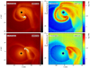 |
Fig. 5 Density and temperature distribution in a slice of the orbital plane of model v10e50 at two consecutive orbital phases. A version without H I cooling is presented in Fig. 12 of Paper I. The time evolution of this density distribution in a co-rotating frame is available as: online movie 1. |
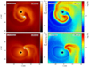 |
Fig. 6 Density and temperature distribution in a slice through the orbital plane of model v05e50 at two consecutive orbital phases. |
4 Accretion disk around the companion
Early 3D SPH simulation studies by Theuns & Jorissen (1993) showed that gravitationally compressed gas around the companion star can form an accretion disk, if the temperature and pressure of the gas surrounding the companion are not too high, so the gas remains bound to the companion star. This is the case in their isothermal EOS (γ = 1), and not in the adiabatic EOS (γ = 1.5) model. They predicted that the formation of a disk will be determined by the efficiency of cooling. In their isothermal models, an inclined accretion disk with a radius of about 1 au forms, with two streams of matter inflow. The inclination of the disk is believed to be due to numerical round-off errors. With the inclusion of more realistic cooling and heating prescriptions, including H I cooling (Spitzer 1978) and rotational H2O cooling (Neufeld & Kaufman 1993), Mastrodemos & Morris (1998) also found that permanent accretion disks form in their models, with radii around 0.6 au. The first higher resolution 3D simulations of disk formation in AGB binaries were conducted by Huarte-Espinosa et al. (2013). They investigated the formation of wind-capture accretion disks in binary systems with orbital separations a ≤ 10 au using an adaptive mesh refinement (AMR) code. They described that accretion disks are able to form because the wind material that will be accreted is not flowing directly towards the companion, but is streaming towards an earlier position, slightly behind the current position of the moving companion. They defined the distance between this off-centre location and the current position of the companion as the accretion line impact parameter,
![Mathematical equation: $\[b=2 \frac{M_{\mathrm{s}}^2\left(M_{\mathrm{s}}+M_{\mathrm{p}}\right)^3}{M_{\mathrm{p}}^5} \frac{\left(\frac{1}{a}\right)^{5 / 2}}{\left(\frac{1}{a}+\frac{1}{r_{\mathrm{w}}}\right)^{7 / 2}},\]$](/articles/aa/full_html/2024/11/aa50338-24/aa50338-24-eq10.png) (5)
(5)
with ![Mathematical equation: $\[r_{\mathrm{w}}=\frac{G M_{\mathrm{p}}}{\left(M_{\mathrm{p}}+M_{\mathrm{s}}\right) v_{\infty}^2}\]$](/articles/aa/full_html/2024/11/aa50338-24/aa50338-24-eq11.png) . The authors concluded that the accretion radius needs to be smaller than b to resolve the formation of the disk. Further, Saladino et al. (2018) performed SPH simulations with a cooling rate following Bowen (1988) and Schure et al. (2009), and found that, in case the terminal wind velocity is smaller than the orbital one (υ∞ < υorb), an accretion disk forms around the companion, but not when υ∞ ≳ υorb. Accretion disks were also modelled in the AMR simulations of El Mellah et al. (2020). They agreed that disks are more likely to form in case of lower wind speed, and showed that the presence of a disk increases the mass accretion efficiency onto the companion, which can lead to a shrinkage of the orbit if the primary is a few times more massive than the companion star. Finally, Lee et al. (2022) modelled wind accretion on a 0.6 M⊙ white dwarf orbiting a giant star at a separation of 2 au, with a similar cooling prescription as Saladino et al. (2018). They found that an accretion disk always forms, regardless of the wind velocity, as long as the accretion radius is sufficiently small and the resolution high enough. They differentiated between two types of disks, depending on whether the wind velocity at the location of the companion in a 1D single star wind is larger or smaller than the orbital velocity of the companion. They found that for a slow wind, the disks have a typical radius of ~0.15 au and an asymmetric density distribution with two inflowing spiral features. Up to > 20% of the mass lost by the AGB star is accreted through the disk onto the companion. For a fast wind, this mass accretion efficiency is lower and consistent with BHL theory. Further, the disks are spatially smaller for increasing wind velocity.
. The authors concluded that the accretion radius needs to be smaller than b to resolve the formation of the disk. Further, Saladino et al. (2018) performed SPH simulations with a cooling rate following Bowen (1988) and Schure et al. (2009), and found that, in case the terminal wind velocity is smaller than the orbital one (υ∞ < υorb), an accretion disk forms around the companion, but not when υ∞ ≳ υorb. Accretion disks were also modelled in the AMR simulations of El Mellah et al. (2020). They agreed that disks are more likely to form in case of lower wind speed, and showed that the presence of a disk increases the mass accretion efficiency onto the companion, which can lead to a shrinkage of the orbit if the primary is a few times more massive than the companion star. Finally, Lee et al. (2022) modelled wind accretion on a 0.6 M⊙ white dwarf orbiting a giant star at a separation of 2 au, with a similar cooling prescription as Saladino et al. (2018). They found that an accretion disk always forms, regardless of the wind velocity, as long as the accretion radius is sufficiently small and the resolution high enough. They differentiated between two types of disks, depending on whether the wind velocity at the location of the companion in a 1D single star wind is larger or smaller than the orbital velocity of the companion. They found that for a slow wind, the disks have a typical radius of ~0.15 au and an asymmetric density distribution with two inflowing spiral features. Up to > 20% of the mass lost by the AGB star is accreted through the disk onto the companion. For a fast wind, this mass accretion efficiency is lower and consistent with BHL theory. Further, the disks are spatially smaller for increasing wind velocity.
To study the accretion disks in our simulations in greater detail, we recomputed our models with a higher resolution and a smaller accretion radius. We decreased the boundary radius Rbound (distance from the AGB sink particle where SPH particles are removed from the simulation) to 20 au to compensate for the large increase in computation time. We changed the value of the (constant) mean molecular weight to μ = 1.26, as we expect the hot accretion region to consist mainly of atomic hydrogen, instead of molecular hydrogen (μ = 2.38) in the larger-scale wind. The effect of changing μ is discussed in Sect. 4.2.
4.1 Resolution study
We performed a resolution study to find the optimal particle resolution and accretion radius to resolve the accretion disk. We first changed the number of particles launched on each sphere around the AGB star (set by iwind_res, see Table B.12 and Siess et al. 2022 for more details), which is equivalent to reducing the mass of the SPH particles. We started our resolution study with model v10e00 for which an accretion disk was present in the simulations in Sect. 3, with iwind_res= 5. Figure B.12 shows a slice of the density distribution in the orbital and meridional plane within au from the companion sink particle after six orbital periods with four different resolutions (iwind_res= 5, 7, 8, 9, corresponding to ~105, 3 × 10⁵, 5 × 10⁵, and 7 × 10⁵ particles, respectively, with the increase from lowest to highest resolution approaching that of a factor of in each direction in 3D grid-based codes). Although this test covers a limited difference in number of particles, due to computational limitations, it shows that increasing the resolution is important to resolve the density structures in and closely around the accretion disk. All characteristic disk features (that are discussed in Sect. 4.3) are resolved from iwind_res= 8 onward. Next, we investigated the effect of decreasing the accretion radius in our models. Following Huarte-Espinosa et al. (2013), to resolve the accretion disk, Rs,accr must be lower than the accretion line impact parameter b (Eq. (5)). This requirement is already fulfilled in our models with Rs,accr = 0.04 au, since for models v20e00, v10e00, and v05e00, b = 0.08, 0.46 and 0.82 au, respectively. However, with this set-up, model v20e00 does not reveal the presence of an accretion disk even when changing the resolution, as illustrated in Fig. B.22, comparing the simulations with iwind_res= 5 and 8 after six orbital periods. However, if we decrease the accretion radius to Rs,accr = 0.01 au = 2.15 R⊙, an accretion disk appears at all the explored resolutions. This can be seen in Fig. B.32 which displays the density distribution for this model with iwind_res= 6, 7, 8. Therefore, we find that the criterion given by Huarte-Espinosa et al. (2013) of rs,accr < b is indeed a necessary, but not a sufficient condition to model the formation of an accretion disk. Our results are in agreement with the conclusion of Lee et al. (2022) that an accretion disk always forms as long as Rs,accr is set small enough. For this model, the higher the resolution, the more confined and the higher the maximum density in the disk becomes. This trend is less obvious in model v10e00 (see Fig. B.12). For model v20e00, the disk might become more confined and denser for higher resolution, but due to computational limits it is not feasible to calculate simulations with Rs,accr = 0.01 au and iwind_res > 8. We therefore conclude that the best set-up for the analysis of accretion disks in our models is an accretion radius of Rs,accr = 0.01 au ≈ 2.15 R⊙ (to ensure that the accretion disk is always present) and a resolution iwind_res set to 8 (to resolve the disk properly), while keeping the computational cost reasonable. The simulations were calculated over ten orbital periods, allowing us to study the evolution over time of the disk mass, size, and mass accretion. With these settings, one model takes approximately four weeks to complete.
4.2 Impact of mean molecular weight choice
As explained before, we changed the mean molecular weight from μ = 2.38 to μ = 1.26 to model the hot accretion region around the companion in an optimal way, considering that μ is not yet self-consistently calculated in our model. However, this has specific implications for the internal energy, u (Eq. (4)), the density distribution and velocity of the wind. To investigate this, we looked at the analytical 1D profiles produced by our PHANTOM models. We concluded that decreasing μ does not significantly change the analytic 1D density, temperature and pressure profile. However, the internal energy, u, increases by a factor of ~2, and the radial wind velocity undergoes a stronger acceleration. Table 3 gives the wind velocity of the 1D models at r = a = 6 au and the terminal velocity υ∞, for the different input velocities, for μ = 2.38 and μ = 1.26. Changing μ from 2.38 to 1.26 makes the 1D wind velocity ~1–3 km s−1 higher at the location of our companion, and adds ~2–4 km s−1 to the terminal velocity, with the largest difference for the lowest input wind velocity. The wind velocity at the location of the companion is one of the prime parameters determining the strength and effects of the wind-companion interaction, so this increase in wind velocity will impact the wind structures and the accretion disk in our simulations. This emphasises the importance of calculating μ self-consistently in future models, so that all regions of the wind can be simultaneously modelled in a physically correct way.
The change in μ in our models leads to a shift in the velocity parameter with respect to the models in Sect. 3. From Table 3 we notice that the velocity profile in model v05e00 with μ = 1.26 adequately resembles the one in model v10e00 with μ = 2.38, and the velocity profile in model v10e00 with μ = 1.26 lies in-between models v10e00 and v20e00 with μ = 2.38.
The density structures surrounding the accretion disks in the orbital plane in the models v05e00, v10e00, and v20e00 with μ = 1.26 are displayed in Fig. 7. As expected from the similar wind velocity profile, the density profile of model v05e00μ,1.26 resembles well the one of model v10e00μ2.38 (Fig. 3). The companion is surrounded by a bow shock spiral in front of the circumstellar disk, and a second flow attached behind the companion. The increased wind velocity due to the decreased μ in model v10e00 results in a weaker wind-companion interaction, such that the companion in model v10e00μ1.26 is surrounded by a weaker bow shock, with a smaller opening angle, compared to model v10e00μ2.38. The velocity shift in model v20e00 is not that large, such that the companion and accretion disk in model v20e00μ1.26 are in front of a two-edged spiral that is very similar to model v20e00μ2.38 (Fig. 1).
Impact of μ on the wind velocity.
4.3 Disk morphology
Figures 8, 9, and 10 display the density distribution, overplotted with the velocity vector field (in the reference frame of the stationary centre-of-mass), of the accretion disk in the orbital plane and in two perpendicular slices for the circular orbit of models v05e00, v10e00, and v20e00, respectively, after ten orbital periods. The orbital plane plots show that the disks consist of high-density material that is rotating counter-clockwise around the companion (prograde with respect to the orbital motion). The perpendicular plane slices reveal the 3D flared shape of the accretion disks, that are aligned with and quasi-symmetric with respect to the orbital plane. As seen in Sect. 3, for low wind velocity, the relatively strong interaction of the companion with the wind produces a bow shock spiral. This bow shock protects the disk from exposure to the wind and thereby from ram pressure stripping, such that it can grow more easily (Lee et al. 2022), as seen in model v05e00 (see left plot in Fig. 7). In model v20e00 there is no bow shock, and in model v10e00 there is the onset of a protecting bow shock (Fig. 7). As a consequence, in Figs. 8, 9, and 10, the disk size is larger for model v05e00, a bit smaller in model v10e00, and significantly smaller for model v20e00. Additionally, in models v05e00 and v10e00, a thin, high-density, spiral-arm structure, that extends counter-clockwise from the flow behind the companion into the accretion disk, is resolved. Material accumulates through this structure behind the companion into the accretion disk (see velocity vectors in Fig. 7). As shown in Fig. 11, that displays the temperature profile in and around the accretion disk for model v05e00, this structure has high temperatures close to 104 K in the orbital plane. Similarly, there is a second high-density structure connecting the accretion disk and the bow shock in front of the companion, making it more difficult to resolve in the density plots. The two structures continue inside the accretion disk and are marked in Fig. C.12 to guide the eye.
The density distribution in the edge-on planes in Figs. 8, 9, and 10 provides an insight in the 3D morphology of the disks, which is not axisymmetric. In models v05e00 and v10e00, the disk has a large flaring angle and reaches large scale heights on the bow shock side (y > 0 in upper right plot of Figs. 8 and 9), whereas on the opposite side (y < 0 in same plot), the disk is less puffy and more confined towards the orbital plane. Moreover, the disk side towards the AGB star (x < 3.6 au in the bottom plot) appears to have a roughly constant flaring angle at increasing distance from the companion, whereas the flaring angle on the side away from the AGB star (x > 3.6 au) seems to increase with radius (best visible at very small radii, close to the location of the companion at x = 3.6 au). The smaller disk in model v20e00 (Fig. 10) is more symmetric, as is expected from the absence of a bow shock, which affects the outer region of the 3D disk morphology in the lower velocity models. These asymmetries are analysed in more detail in Sect. 4.6.
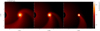 |
Fig. 7 Density distribution in a slice through the orbital plane of models v05e00 (left), v10e00 (middle), and v20e00 (right) with μ = 1.26, Rs,accr = 0.01 au and iwind_res = 8. |
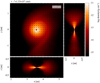 |
Fig. 8 Density distribution in the accretion disk around the companion in model v05e00 (with Rs,accr = 0.01 au and iwind_res = 8) in a slice through the orbital plane (upper left), and in two perpendicular slices (through y = 0 in lower panel, through x = 3.6 in upper right panel). The AGB sink particle is located at y = 0, z = 0, x < 0. Velocity vectors are marked by black arrows on top of the density distribution. |
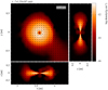 |
Fig. 10 Same as Fig. 8, but for model v20e00. Note that the spatial limits are smaller compared to the accretion disks in models v05e00 and v10e00. |
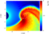 |
Fig. 11 Temperature distribution in a slice through the orbital plane focusing on the accretion disk in model v05e00, of which the estimated radius is marked in white. |
4.4 Quantitative estimates of radius, mass, and scale height
To estimate the radius, r, density scale height, H(r), and mass, Mdisk, of the accretion disks, we adopted a similar method as that of Lee et al. (2022). We integrated the disk structure over radii, ri, with a step Δr = 0.01 au, starting from Rs,accr = 0.01 au (with the origin of the coordinate system at the location of the companion sink particle as in Fig. C.62). For each point (ri, θj, z = 0) in the reference frame of the companion, the density scale height, H(ri, θj), can be calculated on a vertical line through (ri, θj). A theoretical prediction for the vertical density that holds for a thin disk where the gas is isothermal in the z-direction is:
![Mathematical equation: $\[\rho_{\text {theor }}(r, z)=\rho_{\max }(r) e^{-\frac{1}{2}\left(\frac{z}{H}\right)^2}\]$](/articles/aa/full_html/2024/11/aa50338-24/aa50338-24-eq12.png) (6)
(6)
with ρmax the maximum density on the vertical line (generally in the orbital plane, at z = 0, Chiang & Goldreich 1997). On a vertical line through a point (ri, θi), we define two scale heights as
![Mathematical equation: $\[\rho(z=H)=\frac{\rho_{\max }\left(r_i, \theta_j\right)}{\sqrt{e}} \approx 0.60 ~\rho_{\max }\left(r_i, \theta_j\right)\]$](/articles/aa/full_html/2024/11/aa50338-24/aa50338-24-eq13.png) (7)
(7)
and
![Mathematical equation: $\[\rho(z=2 H=\tilde{H})=\frac{\rho_{\max }\left(r_i, \theta_j\right)}{e^2} \approx 0.14 ~\rho_{\max }\left(r_i, \theta_j\right).\]$](/articles/aa/full_html/2024/11/aa50338-24/aa50338-24-eq15.png) (8)
(8)
We estimate the scale height, H(ri, θj), in our simulations as the mean of the absolute values of the positive and negative z-values for which the density drops by a factor of ![Mathematical equation: $\[1 / \sqrt{e}\]$](/articles/aa/full_html/2024/11/aa50338-24/aa50338-24-eq16.png) . Because our disks are not axisymmetric, the density scale height at a given radius, H(ri), is then calculated as the median of ten H(ri, θj) values for equally distributed θj between 0 and 2π. By calculating the median, and not mean value, outlier values are ignored (when other high-density structures are present at certain θj). At each radius ri, the added mass w.r.t. the previous step, M(ri) − M(ri−1), is calculated as the sum of the mass of all SPH particles for which ri−1 < r < ri and |z| <
. Because our disks are not axisymmetric, the density scale height at a given radius, H(ri), is then calculated as the median of ten H(ri, θj) values for equally distributed θj between 0 and 2π. By calculating the median, and not mean value, outlier values are ignored (when other high-density structures are present at certain θj). At each radius ri, the added mass w.r.t. the previous step, M(ri) − M(ri−1), is calculated as the sum of the mass of all SPH particles for which ri−1 < r < ri and |z| < ![Mathematical equation: $\[\tilde{H}\]$](/articles/aa/full_html/2024/11/aa50338-24/aa50338-24-eq17.png) (ri). Note that we use a disk height of
(ri). Note that we use a disk height of ![Mathematical equation: $\[\tilde{H}\]$](/articles/aa/full_html/2024/11/aa50338-24/aa50338-24-eq18.png) (ri), as this provides a more realistic estimate for the total mass in the disk, and has a negligible effect on our estimate of the disk radius. We assume that the disk edge is reached if the relative added mass w.r.t. the previously calculated mass satisfies the following criterion:
(ri), as this provides a more realistic estimate for the total mass in the disk, and has a negligible effect on our estimate of the disk radius. We assume that the disk edge is reached if the relative added mass w.r.t. the previously calculated mass satisfies the following criterion:
![Mathematical equation: $\[\text { if } \frac{M\left(r_i\right)-M\left(r_{i-1}\right)}{M\left(r_{i-1}\right)} \leq 0.3 \frac{\Delta r}{\mathrm{au}} \Longrightarrow r_{\text {disk }} \leq r_i \text {. }\]$](/articles/aa/full_html/2024/11/aa50338-24/aa50338-24-eq19.png) (9)
(9)
The factor of 0.3 in the criterion is the smallest constant towards which the relative added mass consistently keeps decreasing for all models.
The resulting estimates for the disk radius, rdisk, total disk mass, Mdisk, and scale height estimates at radius rdisk for the circular orbit models are given in Table 4. We find that the lower the wind velocity, the larger the disk radius, scale height and mass estimates, with the most extended disk having a radius rdisk = 0.91 au and a total mass estimated to Mdisk ≈ 10−7 M⊙. This confirms that with decreasing AGB wind velocity, more material can be captured by the companion in the accretion disk, which results in a more massive and extended disk. Note that Mdisk/Ms ≪ 0.1, so no gravitational instabilities and formation of moons or planets is expected (Armitage 2020). Figure 12 shows the evolution of the total disk mass throughout ten orbital periods. The roughly constant disk mass near the end of the simulation indicates that the mass accretion rate into the disk equals the mass accretion rate onto the companion sink particle, which is discussed in more detail in Sect. 4.8.
To get a more quantitative view of the disk shape, Fig. 13 displays the radial profile of the scale height, H(r), the aspect ratio, H(r)/r, and the mid-plane density, ρmax, within the disk (averaged over θ). The density scale height and aspect ratio profiles are similar for all models. The aspect ratio, H(r)/r, increases with r, indicating that the disk is flaring. At the inner rim of the disk, for r ≲ 0.07 au, the aspect ratio shows a strong decrease. This indicates that if the disk would be optically thick, the inner rim might self-shadow the disk. However, the mid-plane density, ρmax, is low in this region.
Disk properties for circular models.
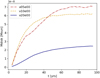 |
Fig. 12 Evolution of the accretion disk mass for the circular orbit binaries. |
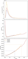 |
Fig. 13 Mid-plane density, ρmax, aspect ratio, H(r)/r, and median density scale height, H(r), (see Eq. (7)) as a function of disk radius for the circular orbit models. The dotted lines in the bottom plot indicate the scale height at the estimated outer disk radius (see Eq. (9)). |
4.5 Disk velocity distribution
Figs. 14 and C.22 display the radial and tangential velocity field, respectively, of the accretion disks in the orbital plane. In contrast to previous figures, the coordinate frame is now the reference frame of the companion, such that the companion sink particle (marked as a black dot) is located at (0, 0, 0) and has a zero-velocity (0, 0, 0), and the AGB star is located at the left side on the y = 0 axis. The estimated radius of the disk (calculated as described in Sect. 4.4) is marked as a dotted circle. In the tangential velocity field plots (Fig. C.22) it can be seen that the material orbiting around the companion is accelerating as it gets closer to the companion. The radial velocity profiles in Fig. 14 are more complex, with material approaching and moving away from the companion on different sides of the disk. This indicates that the particles are on eccentric orbits around the companion, with apastron (periastron) located where υr switches from positive to negative (negative to positive) in the counterclockwise orbit. Interpreting these velocity fields in more detail is not intuitively straight-forward, taking into account that these are the velocities in the co-rotating frame of the moving companion and accretion disk. We note, however, that the tangential velocities are much higher than the radial velocity and will therefore dominate the velocity field. The angular average of the absolute value of the radial velocity as a function of the radial coordinate r is given in Fig. C.32, and shows that |vr| ≪ |υt|.
To understand the general behaviour of particles in this velocity field, Fig. C.42 shows the tangential, υt, and radial velocity distribution, υr, as a function of the radial coordinate, r, averaged over all θ-directions in the orbital plane. The tangential velocity follows very closely a Keplerian rotation in the inner disk up to r ≈ 0.2 au after which the rotation becomes sub-Keplerian. The mean (outward-directed, not absolute value) radial velocity is for most radii close to, but below zero, indicating that material slowly spirals inward while it is rapidly rotating around the companion. Once particles get very close to the companion (r < 0.05 au), within a few accretion radii (Rs,accr = 0.01 au), they are rapidly accreted.
The two spiral-like features that were identified as enhanced density structures in model v05e00, appear in the radial velocity distribution in Fig. 14 as material with lower radial velocity compared to closely surrounding material (so blueshifted in the figure). The spirals are drawn on top of the radial velocity distribution of model v05e00 in Fig. C.52 to guide the eye. This indicates that in these spiral-like structures, material tends to move inward towards the companion sink particle (compared in relation to the surrounding material). The first spiral is visible on the x > 0 side (white-coloured structure in the red velocity area). It initiates behind and goes towards the front of the companion, where it spirals in towards the companion sink particle (y > 0, dark-blue in the blue velocity area). The second spirallike structure initiates in the bow shock in front of the companion (dark blue structure in the blue velocity area at y > 0). In model v20e00, no density enhanced spiral-like feature was resolved in the density distribution (Fig. 10), but the radial velocity distribution in Fig. 14 (right plot) shows that there is a spiral structure with radially in-flowing material. This structure originates from the flow behind the companion, in which material is pulled towards the disk with negative radial velocities up to −40 km s−1, and is visible as a thin blue spiral arising at the lower right-hand side of the disk.
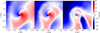 |
Fig. 14 Radial velocity distribution (υr) in accretion disks in models v05e00 (left), v10e00 (middle), and v20e00 (right). The coordinate frame is such that the companion sink particle (marked as a black dot) is located at (0, 0) and has velocity (0, 0, 0), and the AGB star is located at the left side on the y = 0 axis. The estimated radius of the circumstellar disks, as calculated in Sect. 4.4, are marked as a dotted circle. |
4.6 Asymmetries within the accretion disk
From the density plots of Figs. 8 and 9, discussed in Sect. 4.3, we concluded that the bow-shock surrounded disk in the low-velocity models do not have an axisymmetric density distribution. To investigate the asymmetries in more detail, the scale height H(r) (Eq. (7)), aspect ratio H(r)/r, and mid-plane density, ρmax, are calculated separately in four different directions within the disk, θ ∈ [−π/4, π/4], [π/4, 3π/4], [3π/4, 5π/4], [5π/4, 7π/4]. The resulting radial profiles are shown in Figs. 15, C.72, and C.82 for models v05e00, v10e00, and v20e00, respectively. The profiles for model v20e00 are very similar for the different θ regions, confirming the approximately axisymmetric morphology depicted in Fig. 10. For models v05e00 and v10e00, the strongest asymmetry is in the quadrant θ ~ π/2, that corresponds to the front side of the moving companion (y > 0 side, see Fig. C.62). In this region, the scale height, and aspect ratio are larger compared to the median values in the full disk (compare yellow dashed to black solid line in Figs. 15, C.72) because of the onset of the bow shock. The quadrant centred around θ ~ 3π/2, corresponding to the region behind the companion (y < 0 side, see Fig. C.6), has the smallest radial and vertical extent. We additionally note that the disk side towards the AGB star (θ ~ π) appears to have a more constant flaring angle, compared to the stronger increasing flaring angle in the other quadrants. This is reflected in the relatively low and slowly increasing aspect ratio at radii from r ≈ 0.1 to 0.3 au.
4.7 Accretion disks in eccentric orbits
In the eccentric orbit models v05e50, v10e50, and v20e50, the wind-companion interaction is phase-dependent. Therefore the disk morphology and properties change throughout one orbital period, ranging from a larger bow-shock surrounded type, to a smaller symmetric disk type, as well as to in-between phases and more asymmetric shapes.
To see how the accretion disk properties change, Figs. 16, C.92, and 17 visualise the disk at four timesteps within one orbital period for models v05e50, v10e50, and v20e50, respectively. These four timesteps are selected to optimally represent the different disk morphologies that appear during each orbital period. The figures contain (i) the orbital plane density distribution for r ≲ 10 au (top row), (ii) the orbital plane density distribution of the disk in the reference frame of the companion at coordinate (0, 0, 0), with the AGB located on the x < 0, y = 0 axis (as indicate by the arrow, middle row), and (iii) the radial velocity within the disk in the orbital plane, again in the reference frame of the companion (bottom row). Animations of the density distribution during the full last four orbital periods in a co-rotating frame are also available as online movie 2 and 3 for model v05e50 and v20e50, respectively (see Appendix E).
Additionally, estimates of the disk radius, rdisk, mass, Mdisk, and scale heights at these four different phases are given in Tables 5, C.12 and 6 for models v05e50, v10e50, and v20e50, respectively (properties calculated as described in Sect. 4.4).
Models v05e50 and v10e50 behave in a very similar way. Their accretion disk and surrounding structures are influenced by the phase-dependent orbital velocity and distance to the AGB (determining the density of the surrounding wind), and the high-density structures the companion encounters on its orbit. The complex interplay between these effects results in the different disk shapes and velocity profiles visualised in Figs. 16, C.92 and online movie 2. After apastron passage, when the companion approaches the AGB, pronounced spiral density enhancements are present in the disk (see snapshot for t = 85.5 yr), while around periastron passage, when the orbital velocity is maximal, the disk has a strong asymmetry in the density distribution and velocity field (see t = 88.3 yr). Compared to the circular orbit, the disks contain more mass, but are spatially slightly smaller. This is not the case for model v20e50, for which the disk is less massive (Fig. 17). This could be attributed to the fact that in the low-velocity models, the disk encounters a slowly outward moving high-density structure around apastron that can feed the disk (see t = 85.5 and 93 yr in the top row of Fig. 16). The accretion disk surrounded companion seems to collide with the high-density stream in front of its orbital movement direction. In model v20e50, the companion does not encounter such enhanced density structures in the wind, but the structures around the companion do vary from a two-edged spiral (e.g. at t = 86.3 yr) to bow-shock (e.g. at t = 90.6 yr, see top row of Fig. 17 and online movie 3). This also affects the accretion disk shape, as can be seen in the lower two rows of this figure. In this model, the eccentric motion leads to a slightly more extended accretion disk that is less massive than in the circular case (compare Table 6 to Table 4). For all models, the radial velocity field in the vicinity of the companion (bottom row of Figs. 16, C.92, 17) strongly varies over the orbital phases. This shows that the orbit of the particles within the disk and the direction from which material is accreted onto the disk can change rapidly.
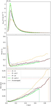 |
Fig. 15 Mid-plane density ρmax, aspect ratio H(r)/r, and density scale height H(r) (Eq. (7)), for model v05e00, at four different θ quadrants centred around θ = 0, π/2, π and 3π/2, and averaged over all θ (full, black line), giving insight into the asymmetric nature of the accretion disk. θ = 0 is the side away from AGB star, as shown in Fig. C.6. |
Disk properties v05e50 at different orbital phases.
Disk properties v20e50 at different orbital phases.
4.8 Mass and angular momentum accretion
In theory, it is expected that in case the local wind velocity is much larger than the orbital velocity, υw ≫ υorb, the Bondi-Hoyle-Lyttleton (BHL) wind accretion scenario (Hoyle & Lyttleton 1939; Bondi & Hoyle 1944) provides a fairly good description of the mass accretion (Theuns et al. 1996). If υw ≪ υorb this is not the case, since the relatively low kinetic energy of the wind increases the impact of the gravitational interaction of the companion on the wind, resulting in a more complex accretion scenario. The theoretical instantaneous BHL mass accretion efficiency is given by
![Mathematical equation: $\[\beta_{\mathrm{BHL}}=\frac{\dot{M}_{\mathrm{acc}}}{\dot{M}_{\mathrm{wind}}}=\alpha_{\mathrm{BHL}}\left(\frac{G M_{\mathrm{s}}}{r v_{\mathrm{w}}^2}\right)^2\left[1+\left(\frac{v_{\mathrm{orb}}}{v_{\mathrm{w}}}\right)^2\right]^{-3 / 2},\]$](/articles/aa/full_html/2024/11/aa50338-24/aa50338-24-eq23.png) (10)
(10)
with αBHL ≈ 0.75 a constant, G the gravitational constant, r the instantaneous orbital separation, υw the estimated local wind velocity at the semi-major axis (r = a) in a single-star model, and ![Mathematical equation: $\[v_{\text {orb }}=\sqrt{G\left(M_{\mathrm{s}}+M_{\mathrm{p}}\right)(2 / r-1 / a)}\]$](/articles/aa/full_html/2024/11/aa50338-24/aa50338-24-eq24.png) the instantaneous relative orbital velocity of the stars with respect to each other. In our models, the estimated local wind velocities are υw ≈ 12.7, 15.0, 22.8 km s−1 for models with initial velocity υini = 5, 10, 20 km s−1 respectively (see Table 3). The relative orbital velocity is υorb ≈ 19 km s−1 in the circular orbits, and varies between 11–33 km s−1 in the eccentric orbits. We do not expect our models to follow the BHL approximation, but it is still valuable to compare our results against these approximations.
the instantaneous relative orbital velocity of the stars with respect to each other. In our models, the estimated local wind velocities are υw ≈ 12.7, 15.0, 22.8 km s−1 for models with initial velocity υini = 5, 10, 20 km s−1 respectively (see Table 3). The relative orbital velocity is υorb ≈ 19 km s−1 in the circular orbits, and varies between 11–33 km s−1 in the eccentric orbits. We do not expect our models to follow the BHL approximation, but it is still valuable to compare our results against these approximations.
The mass accretion efficiency in our models is calculated as the ratio of the mass accreted by the companion sink particle to the mass lost by the AGB star. Table 7 gives the time-averaged BHL mass accretion efficiency calculated over the last two orbital periods, when the wind structures have reached a steady state configuration, from the simulations ⟨βsim⟩ and according to the theory ⟨βBHL⟩. As expected from the relatively low wind velocity compared to the relative orbital velocity, the simulated accretion rates are up to a factor of 2 higher than the theoretical BHL values. The accretion efficiencies vary between ~0.04–0.21, and material is accreted at a higher rate when the wind velocity is lower. Eccentricity is found to increase the average accretion rate, especially in case of a low wind velocity.
To investigate the mass accretion in the eccentric cases in more detail, Fig. 18 displays the phase-dependent calculated and BHL mass accretion efficiency for models v05e50 (top), v10e50 (middle), and v20e50 (bottom). In all models, there is a peak in the accretion efficiency around periastron passage, as the companion passes closer to the AGB star in a higher density region. This accretion peak is sharp because of the high orbital velocity that makes periastron passage short. All models show a secondary peak that is caused by the interaction of the accretion disk with high-density shocks it may encounter every orbital period, or by the interaction of the disk with its surrounding structure that alters between a two-edged flow and a bow shock. These peaks do not occur in the theoretical BHL case, and are inherent to the complex interaction of the companion with the wind structures in the case of υw ≲ υorb.
The mass accreted by the companion carries angular momentum and produces a torque on the stellar companion. The evolution of the torque on the companion star dJs/dt is displayed in Fig. 19 and shows very similar patterns as the mass accretion rate (Fig. 18). In a circular orbit, after convergence of the mass accretion rate, the torque on the companion is almost constant, while in eccentric systems, a main peak appears at apastron followed by a secondary weaker peak when the companion hits over-densities in the flow. In fact, the torque exerted by the accreted matter on the companion can be expressed as
![Mathematical equation: $\[\frac{\mathrm{d} J_{\mathrm{s}}}{\mathrm{~d} t}=\dot{M}_{\mathrm{acc}} j_{\mathrm{acc}},\]$](/articles/aa/full_html/2024/11/aa50338-24/aa50338-24-eq25.png) (11)
(11)
where jacc is the specific angular momentum of the accreted material, and ![Mathematical equation: $\[\dot{M}_{\mathrm{acc}}\]$](/articles/aa/full_html/2024/11/aa50338-24/aa50338-24-eq26.png) the accretion rate onto the companion. Since the companion is surrounded by an accretion disk, we would expect jacc = (dJs/dt)/
the accretion rate onto the companion. Since the companion is surrounded by an accretion disk, we would expect jacc = (dJs/dt)/![Mathematical equation: $\[\dot{M}_{\mathrm{acc}}\]$](/articles/aa/full_html/2024/11/aa50338-24/aa50338-24-eq27.png) to be close to the Keplerian specific angular momentum jK,s = (GMsRs)1/2. Here, Rs is the radius from where orbiting material is being accreted onto the secondary. According to the accretion algorithm (sect 2.8.2 of Price et al. 2018), this radius lies between 0.8 Rs,acc and Rs,acc. In terms of specific angular momentum, this translates into 0.85 ≲ jacc/jK,s ≲ 0.95, indicating that matter is accreted with a high specific angular momentum, close to the Keplerian value. The deviation from the Keplerian value is due to the facts that (i) the accretion radius varies for each particle, and (ii) the disk is not perfectly Keplerian, as attested by the tangential velocity profiles (Fig. C.42) and the presence of spiral arms (Fig. 14). Furthermore, we note that the specific angular momentum jacc slightly increases with increasing wind velocity in the circular systems. This is likely due to the more stable flow in the vicinity of the companion (absence of bow shocks) and higher compactness of the accretion disk (smaller size). As shown by Packet (1981), the accretion of only a few percent of the original companion mass via the disc may spin up the mass accreting star to critical spin velocities, which may impact the global flow structure around the companion. For our simulations, this will be reached after ~104−105 yr.
to be close to the Keplerian specific angular momentum jK,s = (GMsRs)1/2. Here, Rs is the radius from where orbiting material is being accreted onto the secondary. According to the accretion algorithm (sect 2.8.2 of Price et al. 2018), this radius lies between 0.8 Rs,acc and Rs,acc. In terms of specific angular momentum, this translates into 0.85 ≲ jacc/jK,s ≲ 0.95, indicating that matter is accreted with a high specific angular momentum, close to the Keplerian value. The deviation from the Keplerian value is due to the facts that (i) the accretion radius varies for each particle, and (ii) the disk is not perfectly Keplerian, as attested by the tangential velocity profiles (Fig. C.42) and the presence of spiral arms (Fig. 14). Furthermore, we note that the specific angular momentum jacc slightly increases with increasing wind velocity in the circular systems. This is likely due to the more stable flow in the vicinity of the companion (absence of bow shocks) and higher compactness of the accretion disk (smaller size). As shown by Packet (1981), the accretion of only a few percent of the original companion mass via the disc may spin up the mass accreting star to critical spin velocities, which may impact the global flow structure around the companion. For our simulations, this will be reached after ~104−105 yr.
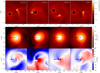 |
Fig. 16 Density distribution in a slice through the orbital plane of model v05e50 at four consecutive orbital phases within one orbital period (top). The centre-of-mass is marked by a white square. The black arrow indicates the direction from the companion to the location of the AGB. Online movie 2 shows the time-evolution of this density distribution during the final four orbital periods of the simulation, in a co-rotating frame. Middle: more zoomed-in density distribution in a slice through the orbital plane at the same four consecutive orbital phases, but the coordinate frame is rotated and translated such that the companion sink particle (shown as a black dot) is located at (0, 0), and the AGB star on the x < 0 side of the y = 0 axis. Bottom panel gives the radial velocity distribution of the accretion disk in model v05e50 at the same timesteps, and in the same coordinate frame as in the middle row. The companion has a zero-velocity (0, 0, 0). The estimated radius of the circumstellar disk (calculated in Sect. 4.4) is shown as a dotted circle in the middle and bottom rows. |
Mean mass accretion efficiency.
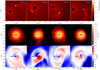 |
Fig. 17 Same as Fig. 16, but for model v20e50. Online movie 3 shows the time-evolution of the orbital plane density distribution during the final four orbital periods of the simulation, in a co-rotating frame. |
5 Further discussion
5.1 The possibilities to resolve or detect accretion disks in observations
The accretion disks in our simulations are small (rdisk < 1 au) and thereby hard to resolve observationally. Additionally, they are relatively hot, with typical temperatures of 6 × 10³−104 K, as can be seen from the temperature distribution in and around the accretion disk of model v05e00 (Fig. 11). Because of the high temperature, the disks are not observable in the submillimetre wavelength range, where AGB outflows are generally observed with facilities such as the Atacama Large Millimeter Array (ALMA). If the disk temperatures in our models are not overestimated, they could be detected through their ultraviolet (UV) excess, which is a wavelength range at which the luminous but cool AGB star is very faint. This is similar to symbiotic systems, in which there is UV emission from a hot white dwarf companion that is accreting matter from the stellar wind of a red giant. This was first suggested by Sahai et al. (2008), who discovered significant far-UV excesses for 9 out of 25 AGB stars observed with GALEX (Galaxy Evolution Explorer), and suggested that this emission is linked to the presence of a binary companion that is either very hot, as in symbiotic systems, or surrounded by a hot accretion disk.
Accretion disks have been detected around post-AGB star companions, through thermal emission in near-infrared (NIR) interferometry by Hillen et al. (2016) and Anugu et al. (2023) with data from the Very Large Telescope / Precision Integrated-Optics Near-infrared Imaging ExpeRiment (VLTI/PIONIER) and the Center for High Angular Resolution Astronomy (CHARA), respectively. Hillen et al. (2016) estimated the temperature of the companion’s accretion disk of the post-AGB binary IRAS 08544-4431 to Tdisk = 4000 ± 2000 K, which is less than the disk temperature in our simulations (T ≈ 6000–10000 K, see Fig. 11). However, De Prins et al. (2024) show that the disk temperature estimate from the NIR observations is underestimated, so the disk emission might peak in the ultraviolet (UV), with inner disk regions as hot as 104 K or more, which is similar to the disks in our simulations. To reliably estimate the temperature distribution of the post-AGB companion’s accretion disk, multi-wavelength interferometric observations are needed.
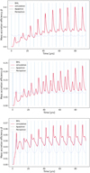 |
Fig. 18 Mass accretion efficiency, β, in models v05e50 (top), v10e50 (middle), and v20e50 (bottom), as calculated from the simulations (red), and compared to the BHL estimates (Eq. (10)). The apastron and peri-astron orbital phases are indicated by vertical lines. |
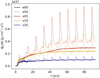 |
Fig. 19 Torque dJs/dt on the companion for the circular (solid line) and eccentric (dotted line) systems. |
5.2 Transition to the post-AGB phase
It is very difficult to model the transition from AGB to the postAGB and PNe phase, and to investigate how the asymmetries and structures that form in the AGB wind will shape the morphologies in later stages. In the post-AGB and (pre-) PN phase, a jet is frequently observed that is launched from an accretion disk around the companion, likely driven by the disk magnetic field (De Prins et al. 2024). In a recent study by Planquart et al. (2024), an accretion disk from which a jet is launched was also discovered around the companion of the AGB binary V Hydrae. The accretion disk around a post-AGB companion may be the descendant of the accretion disk around the AGB companion, that we find in our simulations. However, the accretion disk and jet in post-AGB binaries are believed to by mainly fed by mass streaming from a circumbinary disk (Bollen et al. 2022), instead of from the AGB wind. It is unclear if the accretion disk that forms in AGB binaries does survive the transition to the post-AGB phase, when the feeding mechanism of the companion-surrounding accretion disk changes. Furthermore, it is not entirely clear how the observed post-AGB circumbinary disks form, but they are believed to arise by strong binary interaction before the post-AGB phase (van Winckel et al. 2009). To model the potential formation of circumbinary structures in AGB binaries that might be the progenitors of these post-AGB circumbinary disks, a better treatment of cooling and radiative transfer is needed (Chen et al. 2020).
5.3 Impact of mass-loss rate on wind structures
In the PHANTOM wind model, the wind mass-loss rate is an input parameter, which is set to ![Mathematical equation: $\[\dot{M}\]$](/articles/aa/full_html/2024/11/aa50338-24/aa50338-24-eq28.png) = 10−7 M⊙ yr−1 in our simulations. In Sect. 2.2 we noted that systems with wind velocities of ~20 km s−1 are expected to have higher mass-loss rates. Without the inclusion of H I cooling, the hydrodynamic equations are invariant to a scaling in the mass-loss rate. For completeness, we here shortly investigate the effect of increasing the mass-loss rate in model v20e00 to a more realistic value of
= 10−7 M⊙ yr−1 in our simulations. In Sect. 2.2 we noted that systems with wind velocities of ~20 km s−1 are expected to have higher mass-loss rates. Without the inclusion of H I cooling, the hydrodynamic equations are invariant to a scaling in the mass-loss rate. For completeness, we here shortly investigate the effect of increasing the mass-loss rate in model v20e00 to a more realistic value of ![Mathematical equation: $\[\dot{M}\]$](/articles/aa/full_html/2024/11/aa50338-24/aa50338-24-eq29.png) = 10−5 M⊙ yr−1. For the models analysed in Sect. 3, the increase in mass-loss rate does not affect the wind structures significantly, but leads to an overall increase of the CSE density. In the higher-resolution model with small accretion radius (used to study the accretion disk in Sect. 4), the higher mass-loss rate effects the accretion disk and the surrounding wind structures. Figure C.102 displays the density distribution around the companion in the orbital plane slice for the high-resolution model v20e00, with
= 10−5 M⊙ yr−1. For the models analysed in Sect. 3, the increase in mass-loss rate does not affect the wind structures significantly, but leads to an overall increase of the CSE density. In the higher-resolution model with small accretion radius (used to study the accretion disk in Sect. 4), the higher mass-loss rate effects the accretion disk and the surrounding wind structures. Figure C.102 displays the density distribution around the companion in the orbital plane slice for the high-resolution model v20e00, with ![Mathematical equation: $\[\dot{M}\]$](/articles/aa/full_html/2024/11/aa50338-24/aa50338-24-eq30.png) = 10−5 M⊙ yr−1. Compared to the same model with a lower mass-loss rate (Fig. 10), the disk size and density have increased, and instead of a two-edged spiral, a structure resembling a bow shock forms. The temperature around the companion increased by a factor of ~2, such that the typical temperature within the disk becomes 1.2 × 10⁴−2 × 10⁴ K. For this specific model, an increase in the mass-loss rate by a factor of 100 increases the disk mass by approximately a factor of ~50, the disk radius by a factor of ~1.5 (to 0.6 au), and the scale height with a factor of ~2.3. The mass accretion efficiency slightly decreased from 0.040 to 0.035, such that the effective mass accretion rate increases to 3.5 × 10⁻⁷ M⊙ yr−1.
= 10−5 M⊙ yr−1. Compared to the same model with a lower mass-loss rate (Fig. 10), the disk size and density have increased, and instead of a two-edged spiral, a structure resembling a bow shock forms. The temperature around the companion increased by a factor of ~2, such that the typical temperature within the disk becomes 1.2 × 10⁴−2 × 10⁴ K. For this specific model, an increase in the mass-loss rate by a factor of 100 increases the disk mass by approximately a factor of ~50, the disk radius by a factor of ~1.5 (to 0.6 au), and the scale height with a factor of ~2.3. The mass accretion efficiency slightly decreased from 0.040 to 0.035, such that the effective mass accretion rate increases to 3.5 × 10⁻⁷ M⊙ yr−1.
6 Conclusion
In this work, we use SPH simulations performed with the PHANTOM code to study the effects of atomic H I cooling on the structures that form in the winds of evolved low- and intermediate-mass stars through the interaction with a binary companion. Furthermore, we study the wind-capture accretion discs that form around the companion.
We consider a mass-losing AGB star with a solar-mass companion at an orbital separation of 6 au. Compared to previous simulations done without HI cooling (Malfait et al. 2021), we find that the region surrounding the companion star is efficiently cooled down, with maximum temperatures that are lower by an order of magnitude. This removes the irregularities present in Malfait et al. (2021) and Maes et al. (2021), which were related to a ‘high-energy’ region around the companion and causing irregular or square morphologies and bipolar-like outflows. However, it is still possible to form very asymmetric and complex wind structures, in case of eccentric binary systems in which the kinetic energy of the wind is relatively small compared to the gravitational energy density around the companion. Furthermore, we found that changing the mean molecular weight, μ, in our model impacts the wind velocity profile, which is an important parameter determining which structures form around the companion. This indicates how important it is to self-consistently calculate μ in future models.
Our simulations show that wind material is able to accumulate closely around the companion, forming a high-density accretion disk. The disks consist of material that is orbiting with Keplerian to sub-Keplerian velocities, while slowly moving radially inward towards the companion in a slightly eccentric orbit. The disks are flaring and have radial sizes of ~0.4–0.9 au and disk masses of ~3 × 10⁻⁸−2 × 10⁻⁷ M⊙, with increasing size and radius for decreasing wind velocity. Within the disk, two spiral-like features are identified, having lower radial velocities than the surrounding particles within the disk. In the case of a relatively low wind velocity compared to the orbital velocity, these features also have a relatively high density, making them visible within the disk density distribution. The spiral with the largest density enhancement originates in the wake behind the companion, the second spiral in the bow shock in front of the companion, and they both spiral-in clockwise towards the companion sink particle. In eccentric systems, the disk shape changes throughout an orbital period, due to the phase-dependent wind-companion interaction, and the interaction with other high-density structures present in the inner wind.
The average mass accretion efficiencies in our simulations are up to a factor of ~ two higher than the theoretical BHL predictions, and increase with decreasing velocity and higher eccentricity. The mass accretion rate ranges between 0.04 and 0.21 of the mass loss rate. In the eccentric orbits, there is a mass accretion peak around the close periastron passage, and an additional peak closer around apastron passage. Finally, we found that the companion accretes matter with a high specific angular momentum, close to the Keplerian value, which can result in a significant spin-up of the star.
The small spatial extent of the accretion disks cannot easily be resolved observationally. Furthermore, the disks cannot be observed in the submillimetre wavelength range, where the AGB outflows are typically observed, due to their relatively high temperatures (between ~6000–104 K). If the actual disk temperatures are indeed this high, the disks could be detected through UV flux excess. Such an approach would have to take into account the fact that such UV excess can have a different origin as well, such as accretion onto a hot companion.
Data availability
The input files and final output dumps of the Phantom simulations of this paper, and several movies to illustrate the complex flows within the binary systems, are available online at https://zenodo.org/records/13224218. The movies can be accessed as well at http://www.astro.ulb.ac.be/~siess/Phantom/HIcooling.
Movies associated to Figs. 5, 16 and 17 are available at https://www.aanda.org
Appendices A, B and C are available at: https://zenodo.org/records/13843847
Acknowledgements
We thank Toon De Prins for insightful discussions on accretion disks in post-AGB stars, and we thank Daniel Price for his help concerning the development of PHANTOM. The animations and figures in this paper are made using the visualisation tools Plons3 and SPLASH (Price 2007). JM, ME, and LD acknowledge support from the KU Leuven C1 excellence grant C16/17/007 MAESTRO and the FWO research project G099720N. L.S. is a senior F.N.R.S. research associate. FDC is a postdoctoral research fellow of the Research Foundation – Flanders (FWO), grant 1253223N. LD acknowledges support from the KU Leuven C1 excellence grant BRAVE C16/23/009 and KU Leuven Methusalem grant SOUL METH/24/012.
Appendix A Effect of H I cooling
This appendix is available on Zenodo: https://zenodo.org/records/13843847 and contains additional figures used to study the effect of H I cooling in the phantom model on the wind.
Appendix B Resolution of accretion disks
This appendix is available on Zenodo: https://zenodo.org/records/13843847 and contains an additional table and figures used to study the effect of the resolution of the phantom model on the formation of, and ability to resolve, accretion disks.
Appendix C Structure of accretion disks
This appendix is available on Zenodo: https://zenodo.org/records/13843847 and contains an additional table and figures used to study the structure of accretion disks in our models.
Appendix D Electron number density
Following Palla et al. (1983), we consider the following set of chemical reactions to calculate the electron density:
![Mathematical equation: $\[\begin{aligned}& \mathrm{H}^{+}+\mathrm{e}^{-} \xrightarrow{k_1} \mathrm{H}+\mathrm{h} v, \\& \mathrm{H}+\mathrm{e}^{-} \xrightarrow{k_2} \mathrm{H}^{-}+\mathrm{h} v, \\& \mathrm{H}^{+} \mathrm{H}^{-} \xrightarrow{k_3} \mathrm{H}_2+\mathrm{e}^{-}, \\& \mathrm{H}+\mathrm{H}+\mathrm{H} \underset{k_5}{\stackrel{k_4}{\rightleftharpoons}} \mathrm{H}_2+\mathrm{H}, \\& \mathrm{H}+\mathrm{H}+\mathrm{H}_2 \underset{k_7}{\stackrel{k_6}{\rightleftharpoons}} \mathrm{H}_2+\mathrm{H}_2, \\& \mathrm{H}+\mathrm{e}^{-} \xrightarrow{k_8} \mathrm{H}^{+}+\mathrm{e}^{-}+\mathrm{e}^{-}, \\& \mathrm{H}+\mathrm{H} \xrightarrow{k_9} \mathrm{H}^{+}+\mathrm{e}^{-}+\mathrm{H}.\end{aligned}\]$](/articles/aa/full_html/2024/11/aa50338-24/aa50338-24-eq31.png)
Assuming that all components X = {H, H+, H2, H−, e−} are at equilibrium (∂tX = 0), we obtain the system of equations for the number density of H+, H− and electrons:
![Mathematical equation: $\[n_{\mathrm{H}^{+}}=\frac{k_9 n_{\mathrm{H}}^2+k_8 n_e n_{\mathrm{H}}}{k_1 n_e},\]$](/articles/aa/full_html/2024/11/aa50338-24/aa50338-24-eq32.png) (D.1)
(D.1)
![Mathematical equation: $\[n_{\mathrm{H}^{-}}=\frac{k_2}{k_3} n_e,\]$](/articles/aa/full_html/2024/11/aa50338-24/aa50338-24-eq33.png) (D.2)
(D.2)
![Mathematical equation: $\[\frac{\mathrm{d} n_e}{\mathrm{~d} t}=\frac{\mathrm{d}\left(n_{\mathrm{H}^{+}}-n_{\mathrm{H}^{-}}\right)}{\mathrm{d} t}.\]$](/articles/aa/full_html/2024/11/aa50338-24/aa50338-24-eq34.png) (D.3)
(D.3)
The integration of Eq. (D.3) leads to nH+ = ne + nH-. After substitutions and resolution of a second degree equation, we obtain the following expression for the electron density:
![Mathematical equation: $\[n_e=\frac{\sqrt{4 k_1 k_3 k_9\left(k_2+k_3\right)+k_3^2 k_8^2}+k_3 k_8}{2 k_1\left(k_2+k_3\right)} n_{\mathrm{H}}.\]$](/articles/aa/full_html/2024/11/aa50338-24/aa50338-24-eq35.png) (D.4)
(D.4)
The rate coefficients ki are temperature dependent, except for k3 and are given in Palla et al. (1983). The number of H atoms per unit volume is given by
![Mathematical equation: $\[n_{\mathrm{H}}=\frac{\rho}{m_{\mathrm{H}}\left(1+4 \epsilon_{\mathrm{He}}+..\right)} \approx \frac{\rho}{1.4 ~m_{\mathrm{H}}},\]$](/articles/aa/full_html/2024/11/aa50338-24/aa50338-24-eq36.png)
where εHe is the number of He atom per H atom (εHe ≈ 0.1 for solar composition).
Appendix E Online movies
Movie 1 shows the evolution of the density distribution in the corotating orbital plane of model v10e50. It shows how the structures around the companion in this eccentric binary vary over each orbital period, and how the bow shock interacts and collides with other high density structures. This movie is linked to Fig. 5.
Movie 2 shows the evolution of the density distribution in the corotating orbital plane of model v05e50 during the final four orbital periods of the simulation. This movie focuses on the accretion disk around the companion, and reveals how the accretion disk shape varies throughout one orbital period due to the complex interplay between the phase-dependent wind-companion interaction strength and the interaction of the accretion disk with surrounding high density structures. This movie is linked to Fig. 16.
Movie 3 shows the evolution of the density distribution in the corotating orbital plane of model v20e50 during the final four orbital periods of the simulation. This movie focuses on the accretion disk around the companion, and shows how the surrounding structure varies from a two-edged spiral to bow shock within each orbital period. This movie is appended to Fig. 17.
References
- Akashi, M., & Soker, N. 2017, MNRAS, 469, 3296 [NASA ADS] [CrossRef] [Google Scholar]
- Anugu, N., Kluska, J., Gardner, T., et al. 2023, ApJ, 950, 149 [NASA ADS] [CrossRef] [Google Scholar]
- Armitage, P. J. 2020, Astrophysics of Planet Formation, 2nd edn [CrossRef] [Google Scholar]
- Aydi, E., & Mohamed, S. 2022, MNRAS, 513, 4405 [NASA ADS] [CrossRef] [Google Scholar]
- Balick, B., & Frank, A. 2002, ARA&A, 40, 439 [Google Scholar]
- Bollen, D., Kamath, D., Van Winckel, H., et al. 2022, A&A, 666, A40 [NASA ADS] [CrossRef] [EDP Sciences] [Google Scholar]
- Bondi, H., & Hoyle, F. 1944, MNRAS, 104, 273 [Google Scholar]
- Bowen, G. H. 1988, ApJ, 329, 299 [NASA ADS] [CrossRef] [Google Scholar]
- Chen, Z., Frank, A., Blackman, E. G., Nordhaus, J., & Carroll-Nellenback, J. 2017, MNRAS, 468, 4465 [NASA ADS] [CrossRef] [Google Scholar]
- Chen, Z., Ivanova, N., & Carroll-Nellenback, J. 2020, ApJ, 892, 110 [NASA ADS] [CrossRef] [Google Scholar]
- Chiang, E. I., & Goldreich, P. 1997, ApJ, 490, 368 [Google Scholar]
- Corporaal, A., Kluska, J., Van Winckel, H., Kamath, D., & Min, M. 2023, A&A, 671, A15 [NASA ADS] [CrossRef] [EDP Sciences] [Google Scholar]
- Danilovich, T., Malfait, J., Van de Sande, M., et al. 2024, Nat. Astron., 8, 308 [CrossRef] [Google Scholar]
- De Marco, O. 2009, PASP, 121, 316 [NASA ADS] [CrossRef] [Google Scholar]
- De Marco, O., Passy, J.-C., Frew, D. J., Moe, M., & Jacoby, G. H. 2013, MNRAS, 428, 2118 [NASA ADS] [CrossRef] [Google Scholar]
- De Prins, T., Van Winckel, H., Ferreira, J., et al. 2024, A&A, 689, A151 [NASA ADS] [CrossRef] [EDP Sciences] [Google Scholar]
- Decin, L. 2021, ARA&A, 59, 337 [NASA ADS] [CrossRef] [Google Scholar]
- Decin, L., Montargès, M., Richards, A. M. S., et al. 2020, Science, 369, 1497 [Google Scholar]
- El Mellah, I., Bolte, J., Decin, L., Homan, W., & Keppens, R. 2020, A&A, 637, A91 [NASA ADS] [CrossRef] [EDP Sciences] [Google Scholar]
- Escorza, A., Karinkuzhi, D., Jorissen, A., et al. 2019, A&A, 626, A128 [NASA ADS] [CrossRef] [EDP Sciences] [Google Scholar]
- Esseldeurs, M., Siess, L., De Ceuster, F., et al. 2023, A&A, 674, A122 [NASA ADS] [CrossRef] [EDP Sciences] [Google Scholar]
- García-Segura, G., Ricker, P. M., & Taam, R. E. 2018, ApJ, 860, 19 [CrossRef] [Google Scholar]
- Hillen, M., Kluska, J., Le Bouquin, J. B., et al. 2016, A&A, 588, L1 [NASA ADS] [CrossRef] [EDP Sciences] [Google Scholar]
- Höfner, S., & Olofsson, H. 2018, A&A Rev., 26, 1 [CrossRef] [Google Scholar]
- Homan, W., Montargès, M., Pimpanuwat, B., et al. 2020, A&A, 644, A61 [NASA ADS] [CrossRef] [EDP Sciences] [Google Scholar]
- Hoyle, F., & Lyttleton, R. A. 1939, Proc. Camb. Philos. Soc., 35, 405 [CrossRef] [Google Scholar]
- Huarte-Espinosa, M., Carroll-Nellenback, J., Nordhaus, J., Frank, A., & Blackman, E. G. 2013, MNRAS, 433, 295 [NASA ADS] [CrossRef] [Google Scholar]
- Jones, D., & Boffin, H. M. J. 2017, Nat. Astron., 1, 0117 [Google Scholar]
- Jorissen, A., Boffin, H. M. J., Karinkuzhi, D., et al. 2019, A&A, 626, A127 [NASA ADS] [CrossRef] [EDP Sciences] [Google Scholar]
- Kervella, P., Homan, W., Richards, A. M. S., et al. 2016, A&A, 596, A92 [NASA ADS] [CrossRef] [EDP Sciences] [Google Scholar]
- Kim, H., & Taam, R. E. 2012, ApJ, 759, 59 [Google Scholar]
- Kim, H., Liu, S.-Y., & Taam, R. E. 2019, ApJS, 243, 35 [Google Scholar]
- Lee, Y.-M., Kim, H., & Lee, H.-W. 2022, ApJ, 931, 142 [NASA ADS] [CrossRef] [Google Scholar]
- Liu, Z.-W., Stancliffe, R. J., Abate, C., & Matrozis, E. 2017, ApJ, 846, 117 [Google Scholar]
- Lora, V., Toalá, J. A., González-Carbajal, J. I., et al. 2023, MNRAS, 522, 3337 [NASA ADS] [CrossRef] [Google Scholar]
- Maercker, M., Mohamed, S., Vlemmings, W. H. T., et al. 2012, Nature, 490, 232 [NASA ADS] [CrossRef] [Google Scholar]
- Maes, S., Homan, W., Malfait, J., et al. 2021, A&A, 653, A25 [NASA ADS] [CrossRef] [EDP Sciences] [Google Scholar]
- Malfait, J., Homan, W., Maes, S., et al. 2021, A&A, 652, A51 (Paper I) [NASA ADS] [CrossRef] [EDP Sciences] [Google Scholar]
- Mastrodemos, N., & Morris, M. 1998, ApJ, 497, 303 [Google Scholar]
- Mastrodemos, N., & Morris, M. 1999, ApJ, 523, 357 [Google Scholar]
- Mauron, N., & Huggins, P. J. 2006, A&A, 452, 257 [NASA ADS] [CrossRef] [EDP Sciences] [Google Scholar]
- Millar, T. J. 2004, Molecule and Dust Grain Formation, 247 [Google Scholar]
- Moe, M., & Di Stefano, R. 2017, ApJS, 230, 15 [Google Scholar]
- Neufeld, D. A., & Kaufman, M. J. 1993, ApJ, 418, 263 [NASA ADS] [CrossRef] [Google Scholar]
- Offner, S. S. R., Moe, M., Kratter, K. M., et al. 2023, in Astronomical Society of the Pacific Conference Series, 534, Protostars and Planets VII, eds. S. Inutsuka, Y. Aikawa, T. Muto, K. Tomida, & M. Tamura, 275 [Google Scholar]
- Oomen, G.-M., Van Winckel, H., Pols, O., et al. 2018, A&A, 620, A85 [NASA ADS] [CrossRef] [EDP Sciences] [Google Scholar]
- Packet, W. 1981, A&A, 102, 17 [NASA ADS] [Google Scholar]
- Palla, F., Salpeter, E. E., & Stahler, S. W. 1983, ApJ, 271, 632 [NASA ADS] [CrossRef] [Google Scholar]
- Planquart, L., Jorissen, A., Escorza, A., Verhamme, O., & Van Winckel, H. 2024, A&A, 682, A143 [NASA ADS] [CrossRef] [EDP Sciences] [Google Scholar]
- Price, D. J. 2007, PASA, 24, 159 [Google Scholar]
- Price, D. J., Wurster, J., Tricco, T. S., et al. 2018, PASA, 35, e031 [Google Scholar]
- Ramos-Larios, G., Santamaría, E., Guerrero, M. A., et al. 2016, MNRAS, 462, 610 [NASA ADS] [CrossRef] [Google Scholar]
- Ramstedt, S., Mohamed, S., Vlemmings, W. H. T., et al. 2014, A&A, 570, L14 [NASA ADS] [CrossRef] [EDP Sciences] [Google Scholar]
- Ramstedt, S., Vlemmings, W. H. T., Doan, L., et al. 2020, A&A, 640, A133 [EDP Sciences] [Google Scholar]
- Sahai, R., Findeisen, K., Gil de Paz, A., & Sánchez Contreras, C. 2008, ApJ, 689, 1274 [NASA ADS] [CrossRef] [Google Scholar]
- Saladino, M. I., Pols, O. R., van der Helm, E., Pelupessy, I., & Portegies Zwart, S. 2018, A&A, 618, A50 [NASA ADS] [CrossRef] [EDP Sciences] [Google Scholar]
- Saladino, M. I., Pols, O. R., & Abate, C. 2019, A&A, 626, A68 [NASA ADS] [CrossRef] [EDP Sciences] [Google Scholar]
- Schure, K. M., Kosenko, D., Kaastra, J. S., Keppens, R., & Vink, J. 2009, A&A, 508, 751 [NASA ADS] [CrossRef] [EDP Sciences] [Google Scholar]
- Siess, L., Homan, W., Toupin, S., & Price, D. J. 2022, A&A, 667, A75 [NASA ADS] [CrossRef] [EDP Sciences] [Google Scholar]
- Spitzer, L. 1978, Physical processes in the interstellar medium [Google Scholar]
- Theuns, T., & Jorissen, A. 1993, MNRAS, 265, 946 [Google Scholar]
- Theuns, T., Boffin, H. M. J., & Jorissen, A. 1996, MNRAS, 280, 1264 [Google Scholar]
- Tielens, A. G. G. M. 2005, The Physics and Chemistry of the Interstellar Medium (Cambridge University Press) [Google Scholar]
- Toonen, S., Nelemans, G., & Portegies Zwart, S. 2012, A&A, 546, A70 [NASA ADS] [CrossRef] [EDP Sciences] [Google Scholar]
- Van Winckel, H. 2003, ARA&A, 41, 391 [Google Scholar]
- van Winckel, H., Lloyd Evans, T., Briquet, M., et al. 2009, A&A, 505, 1221 [NASA ADS] [CrossRef] [EDP Sciences] [Google Scholar]
- Verhamme, O., Kluska, J., Ferreira, J., et al. 2024, A&A, 684, A79 [NASA ADS] [CrossRef] [EDP Sciences] [Google Scholar]
Appendix available on Zenodo: https://zenodo.org/records/13843847
Appendix available on Zenodo: https://zenodo.org/records/13843847
Appendix available on Zenodo: https://zenodo.org/records/13843847
Appendix available on Zenodo: https://zenodo.org/records/13843847
Appendix available on Zenodo: https://zenodo.org/records/13843847
Appendix available on Zenodo: https://zenodo.org/records/13843847
Appendix available on Zenodo: https://zenodo.org/records/13843847
Appendix available on Zenodo: https://zenodo.org/records/13843847
Appendix available on Zenodo: https://zenodo.org/records/13843847
All Tables
All Figures
|
Fig. 1 Density profile in a slice through (top row) and perpendicular to (bottom row) the orbital plane of binary models v20e00 (left), v10e00 (middle), and v05e00 (right) at the end of the simulation (t = 93 yr), with log = (log10). The AGB and companion star are marked as the left and right dot, respectively, not to scale. In the upper left panel, the ‘backward spiral edge’ (BSE), the ‘frontward spiral edge’ (FSE), and the location where they merge into one spiral structure are indicated. A version without H I cooling is presented in Fig. 1 in Paper I. |
| In the text | |
|
Fig. 2 Velocity profile in a slice through the orbital plane (left) and analytical Archimedean spiral fit of the merging ‘backward spiral edge’ (BSE) and ‘frontward spiral edge’ (FSE) of model v20e00 (right). A version without H I cooling is presented in Figs. 2 and 3 of Paper I. |
| In the text | |
|
Fig. 3 Density, velocity, temperature, and pressure profile in the orbital plane of model v10e00, superimposed with the velocity vector profile which is shown as black arrows. A version without H I cooling is presented in Fig. 4 of Paper I. |
| In the text | |
|
Fig. 4 Density distribution in a slice through the orbital plane (left, x-y plane) and in two perpendicular meridional plane slices (middle, x-z plane, and right, y-z plane) of the three eccentric binary models v20e50 (top), v10e50 (middle) and v05e50 (bottom). The white arrows indicate low-density gaps (darker regions in figure), and the white circles annotate some of the bifurcations (at edges of low-density gaps). A version without H I cooling is presented in Fig. 6 (v20e50, right column), Fig. 10 (v10e50, second row), and Fig. 13 (v05e50, third row) of Paper I. |
| In the text | |
|
Fig. 5 Density and temperature distribution in a slice of the orbital plane of model v10e50 at two consecutive orbital phases. A version without H I cooling is presented in Fig. 12 of Paper I. The time evolution of this density distribution in a co-rotating frame is available as: online movie 1. |
| In the text | |
|
Fig. 6 Density and temperature distribution in a slice through the orbital plane of model v05e50 at two consecutive orbital phases. |
| In the text | |
|
Fig. 7 Density distribution in a slice through the orbital plane of models v05e00 (left), v10e00 (middle), and v20e00 (right) with μ = 1.26, Rs,accr = 0.01 au and iwind_res = 8. |
| In the text | |
|
Fig. 8 Density distribution in the accretion disk around the companion in model v05e00 (with Rs,accr = 0.01 au and iwind_res = 8) in a slice through the orbital plane (upper left), and in two perpendicular slices (through y = 0 in lower panel, through x = 3.6 in upper right panel). The AGB sink particle is located at y = 0, z = 0, x < 0. Velocity vectors are marked by black arrows on top of the density distribution. |
| In the text | |
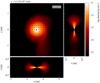 |
Fig. 9 Same as Fig. 8, but for model v10e00. |
| In the text | |
|
Fig. 10 Same as Fig. 8, but for model v20e00. Note that the spatial limits are smaller compared to the accretion disks in models v05e00 and v10e00. |
| In the text | |
|
Fig. 11 Temperature distribution in a slice through the orbital plane focusing on the accretion disk in model v05e00, of which the estimated radius is marked in white. |
| In the text | |
|
Fig. 12 Evolution of the accretion disk mass for the circular orbit binaries. |
| In the text | |
|
Fig. 13 Mid-plane density, ρmax, aspect ratio, H(r)/r, and median density scale height, H(r), (see Eq. (7)) as a function of disk radius for the circular orbit models. The dotted lines in the bottom plot indicate the scale height at the estimated outer disk radius (see Eq. (9)). |
| In the text | |
|
Fig. 14 Radial velocity distribution (υr) in accretion disks in models v05e00 (left), v10e00 (middle), and v20e00 (right). The coordinate frame is such that the companion sink particle (marked as a black dot) is located at (0, 0) and has velocity (0, 0, 0), and the AGB star is located at the left side on the y = 0 axis. The estimated radius of the circumstellar disks, as calculated in Sect. 4.4, are marked as a dotted circle. |
| In the text | |
|
Fig. 15 Mid-plane density ρmax, aspect ratio H(r)/r, and density scale height H(r) (Eq. (7)), for model v05e00, at four different θ quadrants centred around θ = 0, π/2, π and 3π/2, and averaged over all θ (full, black line), giving insight into the asymmetric nature of the accretion disk. θ = 0 is the side away from AGB star, as shown in Fig. C.6. |
| In the text | |
|
Fig. 16 Density distribution in a slice through the orbital plane of model v05e50 at four consecutive orbital phases within one orbital period (top). The centre-of-mass is marked by a white square. The black arrow indicates the direction from the companion to the location of the AGB. Online movie 2 shows the time-evolution of this density distribution during the final four orbital periods of the simulation, in a co-rotating frame. Middle: more zoomed-in density distribution in a slice through the orbital plane at the same four consecutive orbital phases, but the coordinate frame is rotated and translated such that the companion sink particle (shown as a black dot) is located at (0, 0), and the AGB star on the x < 0 side of the y = 0 axis. Bottom panel gives the radial velocity distribution of the accretion disk in model v05e50 at the same timesteps, and in the same coordinate frame as in the middle row. The companion has a zero-velocity (0, 0, 0). The estimated radius of the circumstellar disk (calculated in Sect. 4.4) is shown as a dotted circle in the middle and bottom rows. |
| In the text | |
|
Fig. 17 Same as Fig. 16, but for model v20e50. Online movie 3 shows the time-evolution of the orbital plane density distribution during the final four orbital periods of the simulation, in a co-rotating frame. |
| In the text | |
|
Fig. 18 Mass accretion efficiency, β, in models v05e50 (top), v10e50 (middle), and v20e50 (bottom), as calculated from the simulations (red), and compared to the BHL estimates (Eq. (10)). The apastron and peri-astron orbital phases are indicated by vertical lines. |
| In the text | |
|
Fig. 19 Torque dJs/dt on the companion for the circular (solid line) and eccentric (dotted line) systems. |
| In the text | |
Current usage metrics show cumulative count of Article Views (full-text article views including HTML views, PDF and ePub downloads, according to the available data) and Abstracts Views on Vision4Press platform.
Data correspond to usage on the plateform after 2015. The current usage metrics is available 48-96 hours after online publication and is updated daily on week days.
Initial download of the metrics may take a while.