| Issue |
A&A
Volume 691, November 2024
|
|
|---|---|---|
| Article Number | A192 | |
| Number of page(s) | 13 | |
| Section | Stellar structure and evolution | |
| DOI | https://doi.org/10.1051/0004-6361/202449646 | |
| Published online | 13 November 2024 | |
Revised spin for the black hole in GRS 1716-249 given a new distance determination
1
Key Laboratory of Particle Astrophysics, Institute of High Energy Physics, Chinese Academy of Sciences, Beijing 100049, China
2
University of Chinese Academy of Sciences, Chinese Academy of Sciences, Beijing 100049, China
⋆ Corresponding authors; This email address is being protected from spambots. You need JavaScript enabled to view it.
; This email address is being protected from spambots. You need JavaScript enabled to view it.
; This email address is being protected from spambots. You need JavaScript enabled to view it.
Received:
17
February
2024
Accepted:
14
September
2024
Abstract
GRS 1716–249 is a stellar-mass black hole in a low-mass X-ray binary that underwent a giant outburst in 2016–17. In this paper, we use simultaneous observations from the Hard X-ray Modulation Telescope (Insight-HXMT) and the Nuclear Spectroscopic Telescope Array (NuSTAR) to determine its basic parameters. The observations were performed during the softest part of the outburst and the spectra show clear thermal disk emission and reflection features. We fit the X-ray energy spectra using the joint fitting method of the continuum and reflection components with the kerrbb2 + relxill model. Since there is a possibility that the distance to this source was previously underestimated, we used the latest distance parameter of 6.9 kpc in our study, in contrast to previous works, where the distance was set at 2.4 kpc. Through a spectral fitting of the black hole mass at 6.4 M⊙, we observe a strong dependence of the derived spin on the distance: a* = 0.972−0.005+0.004 at an assumed distance of 2.4 kpc and a∗ = 0.464−0.007+0.016 at an assumed distance of 6.9 kpc, at a confidence level of 90%. When considering the uncertainties in the distance and black hole mass, there will be a wider range of spin with a*< 0.78. The fitting results with the new distance indicate that GRS 1716–249 harbors a moderate spin black hole with an inclined (i ∼ 40 − 50°) accretion disk around it. Additionally, we have also found that solely using the method of reflection component fitting, while ignoring the constraints on the spin from the accretion disk component will result in an extremely high spin.
Key words: accretion / accretion disks / black hole physics / stars: individual: GRS 1716-249 / X-rays: binaries
© The Authors 2024
 Open Access article, published by EDP Sciences, under the terms of the Creative Commons Attribution License (https://creativecommons.org/licenses/by/4.0), which permits unrestricted use, distribution, and reproduction in any medium, provided the original work is properly cited.
This article is published in open access under the Subscribe to Open model. This email address is being protected from spambots. You need JavaScript enabled to view it. to support open access publication.
1. Introduction
Spin is an important parameter of a black hole (BH) and, together with its mass, it can be used to determine the spacetime around it. Spin influences the accretion of matter and the formation of jets (for a review, see Reynolds 2021). Generally, the BH spin, a*, is defined as a* = Jc/GM2, where J represents the angular momentum of the black hole, G stands for the gravitational constant, and c denotes the speed of light. The magnitude of the spin determines the radius of the innermost stable circular orbit (ISCO), RISCO. A larger value of a* corresponds to a smaller RISCO. For example, when a* = 0 (Schwarzschild black hole), RISCO is equal to 6 Rg (where Rg = GM/c2 is called the gravitational radius); when a* = 1 (extreme Kerr black hole), RISCO is equal to 1 Rg. Currently, there are two main methods for measuring black hole spin through spectral fitting: continuum fitting (Zhang et al. 1997; McClintock et al. 2014) and reflection component fitting (Fabian et al. 1989; Reynolds & Fabian 2008; García et al. 2014, 2018a). Both methods commonly require the inner edge of the accretion disk to be located at the position of the ISCO (Rin = RISCO).
According to the standard accretion disk theory (Shakura & Sunyaev 1973; Novikov & Thorne 1973), the spin of a black hole affects the temperature of the inner disk, which, in turn, affects the thermal emission of the accretion disk. The method of continuum fitting is precisely used to constrain the spin of the black hole by fitting the spectrum of the disk. However, the use of this method requires that the distance to the source (D), the inclination of the accretion disk (i), and the mass of the black hole (MBH) are known (the reasons can be found in McClintock et al. 2011). Two commonly used models for fitting the disk component are kerrbb (Li et al. 2005) and kerrbb2 (McClintock et al. 2006), which consider the full relativistic effects. The key fitting parameters of these models include the black hole spin and the mass accretion rate (Ṁ).
The typical reflection features are the iron line (at ∼6–7 keV) and the Compton hump (at ∼20–30 keV). The iron line emitted from the inner disk close to the black hole is influenced by the Doppler effect, relativistic beaming effect, and gravitational redshift, resulting in a broadened and distorted profile (Reynolds & Nowak 2003; Miller 2007). The gravitational redshift mainly affects the red wing of the iron line. The larger the black hole spin, the further the red wing extends to lower energies. This is because a larger spin allows the inner disk to be closer to the black hole and experience a stronger gravitational potential well. The main aim of the reflection component fitting is to obtain the profile of the iron line. This method does not depend on MBH and D and can also be used to constrain i.
In theory, there are billions of stellar-mass black holes in the Milky Way galaxy (Brown & Bethe 1994). However, there are only around twenty X-ray binary systems containing a dynamically confirmed black hole (Remillard & McClintock 2006; Özel et al. 2010; Corral-Santana et al. 2016), and GRS 1716–249 is was discovered in 1993 by the Compton Gamma Ray Observatory (CGRO)/BATSE and Granat/SIGMA telescopes (Harmon et al. 1993; Ballet et al. 1993). After about 23 years of quiescence, GRS 1716–249 had another outburst detected by Monitor of All-sky X-ray Image (MAXI) on December 18, 2016 (Negoro et al. 2016). During this outburst, when the source was in the hard intermediate state, it is believed that the accretion disk was a standard disk with the inner edge located at the ISCO (Bassi et al. 2019). Additionally, the spectrum showed significant power-law (PL) components from the corona, as well as prominent reflection features (broad iron line and Compton hump) (Bassi et al. 2019; Tao et al. 2019). Therefore, this source presents an ideal case for measuring the black hole spin because both the continuum fitting and reflection component fitting methods can be combined to simultaneously constrain the parameters of the black hole.
The system parameters of this source, especially the distance, have not been well constrained. della Valle et al. (1994) estimated the distance to be 2.2–2.8 kpc, while Masetti et al. (1996) provided a lower limit on the black hole mass of 4.9 M⊙, a companion star mass of ∼1.6 M⊙, an orbital period of ∼14.7 hr, and a distance of 2.4 ± 0.4 kpc. By fixing the distance at 2.4 kpc, Tao et al. (2019) found the black hole spin of a* > 0.92, the accretion disk inclination of i ∼ 40 − 50°, and the black hole mass of MBH< 8 M⊙, and Chatterjee et al. (2021) used a two-component advective flow (TCAF) model to constrain the black hole mass to be between 4.5–5.9 M⊙. However, Saikia et al. (2022) argued that the distance of 2.4 kpc is an underestimate. They conservatively estimated the distance of GRS 1716–249 to be 4–17 kpc based on the global optical/X-ray correlation and suggested a most likely value of D ∼ 4–8 kpc based on the dynamics of the binary system. Casares et al. (2023) presented evidence for a 6.7 hr orbital period and used the empirical relationship between the quiescent r-band magnitude and the orbital period to constrain the distance to 6.9 ± 1.1 kpc, consistent with the results given by Saikia et al. (2022). Furthermore, Casares et al. (2023) also provided an orbital inclination of 61 ± 15° and a BH mass of  ,M⊙ at 68% confidence.
Due to the distance-dependent nature of continuum fitting methods, different distances may yield different spin measurement results. Therefore, in this paper, we used two different distance parameters: the previously applied 2.4 kpc (Masetti et al. 1996) and the most recent 6.9 kpc provided by Casares et al. (2023), to highlight the impact of distance changes on spin measurements. We employed a joint fitting method using continuum and reflection spectra to constrain the spin, utilizing data from the Hard X-ray Modulation Telescope (Insight-HXMT) and the Nuclear Spectroscopic Telescope Array (NuSTAR) simultaneous observations during the hard intermediate state in the 2016–2017 outbrst. In the following (Sect. 2), we describe the observations and data reduction. Section 3 presents the spectral fitting and results. Our results are discussed in Sect. 4 and summarized in Sect. 5.
2. Observations and data reduction
In contrast to Tao et al. (2019), who utilized simultaneous the Neil Gehrels Swift Observatory (Swift) and NuSTAR data, in this study, we use simultaneous Insight-HXMT and NuSTAR data. Insight-HXMT can provide high-statistics spectra up to 150 keV for this source, enabling us to place effective constraints on the PL and reflection components. In addition, the lower energy limit of 1 keV for Insight-HXMT affords an accurate modeling of the disk component. Moreover, unlike the Swift data used by Tao et al. (2019), the spectra are not prone to distortion due to pile-up effects, as Insight-HXMT does not suffer from this issue.
Insight-HXMT observed GRS 1716–249 twice during the 2016–2017 outburst. According to the spectral classification of Bassi et al. (2019), both observations are in the hard intermediate state. NuSTAR observed the source three times in the hard intermediate state. The second observation by Insight-HXMT (obsID P0114335002) is strictly simultaneous with the third NuSTAR observation (obsID 90301007002), which started on July 28, 2017 and ended on July 30, 2017. The simultaneous observations by Insight-HXMT and NuSTAR are indicated on the outburst light curve obtained from MAXI/GSC (see Fig. 1). The effective exposure times for Insight-HXMT/LE and NuSTAR/FPMA are 26 ks and 89 ks, respectively (see Table 1). Since the observation span exceeds two days and the source’s luminosity, that is, accretion rate, changes drastically during this period, we split the observations of Insight-HXMT and NuSTAR into two datasets (see Fig. 2) to more accurately measure the spin. The information on the divided data is provided in Table 2.
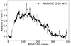 |
Fig. 1. MAXI/GSC light-curve (2–20 keV) of GRS 1716–249. The solid red vertical line represents the simultaneous Insight-HXMT and NuSTAR observations used in this work. |
Observation information on Insight-HXMT and NuSTAR
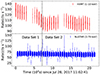 |
Fig. 2. Light curves of Insight-HXMT/LE (top pannel) and NuSTAR/FPMA (bottom panel). The black dashed vertical line represents the division point for both datasets. |
Information on datasets 1 and 2.
2.1. Insight-HXMT
We performed a data reduction using the Insight-HXMT Data Analysis Software (HXMTDASv2.051) and the calibration database files (CALDB v2.06). To determine the appropriate time intervals, we established the following criteria: (a) pointing offset angle should be less than 0.04°; (b) Earth elevation angle should be greater than 10°; (c) there should be a minimum time interval of 300 s from the crossing of the South Atlantic Anomaly region; and (d) the geomagnetic cutoff rigidity should exceed 8 GV. The background for the Low Energy (LE), Medium Energy (ME), and High Energy (HE) telescopes were generated using the scripts lebkgmap, mebkgmap, and hebkgmap, respectively, based on the Insight-HXMT background models (Liao et al. 2020a; Guo et al. 2020; Liao et al. 2020b). The response files for LE, ME, and HE were generated using lerspgen, merspgen, and herspgen, respectively. Following the recommendation of the Insight-HXMT calibration group, the combined spectra are rebinned as follows: The spectra of LE, ME, and HE are respectively rebinned with 1000, 800, and 600 counts per bin at least. Additionally, systematic errors of 1%, 1%, and 2% were applied to the LE, ME, and HE spectra, respectively.
2.2. NuSTAR
The nupipeline routine of NuSTARDAS v1.9.7 in HEASoft v6.29, with CALDB v20211115, was employed to process the cleaned event files. The nuproducts tool is then used to extract the source events, by adopting a circular region surrounding the source with a radius of 80″ to optimize the signal-to-noise ratio (S/N) of the spectra2. The corresponding background extraction region is a nearby source-free circle with a radius of 80″. The spectra were rebinned with 50 counts per bin at least.
3. Analysis and results
To obtain more reliable results, we performed a joint fit of the spectra from datasets 1 and 2. The energy bands used for Insight-HXMT data are 1–7 keV for LE, 10–35 keV for ME, and 35–150 keV for HE. For NuSTAR, we selected the energy band of 3–79 keV. The spectral fitting was conducted using XSPEC v12.12.0 (Arnaud 1996). The abundances were set to WILM (Wilms et al. 2000), and the cross-sections were set to VERN (Verner et al. 1996). All errors are estimated via the Markov chain Monte Carlo algorithm (MCMC) with a length of 600 000.
Due to the source being in the hard intermediate state (Bassi et al. 2019), where the spectra exhibit prominent disk emission and reflection features (Tao et al. 2019), we performed a joint fitting of the spectra using both a continuum and reflection spectral model. The model selected for the fitting is tbabs*(kerrbb+relxill). Additionally, a multiplicative constant model (constant) was included to account for the normalization discrepancies between different telescopes. Therefore, our fitting model is M1 = constant*tbabs*(kerrbb+relxill), as shown in Table A.1. The kerrbb model is a multi-temperature blackbody model that describes the spectrum emitted by a geometrically thin, steady-state accretion disk around a Kerr black hole, taking into account full relativistic effects (Li et al. 2005). The relxill3 model is a relativistic disk coronal reflection model that describes the reflection produced by the corona (with a cutoff PL spectrum) illuminating the inner regions of the accretion disk (Dauser et al. 2014; García et al. 2014). In the kerrbb model, we fixed the BH mass at 6.4 M⊙ (Casares et al. 2023) and the normalization at 1, and we linked the BH spin (a*) and the disk inclination (i) to that of relxill. In the relxill model, we fixed the inner radius of the accretion disk (Rin) to −1, since the disk inner edge is at the ISCO (Bassi et al. 2019), and presumed that within the range from Rin to a specific break radius (Rb), the emissivity is defined by a single inner emissivity index (qin); beyond Rb, it generally adopts the standard r−3 (qout = 3) profile. For different datasets, some parameters were linked and allowed to vary freely, including the X-ray absorption column density (NH), a*, i, and iron abundance (AFe). Other parameters are independent between different datasets, such as the mass accretion rate (Ṁ) and the spectral hardening factor, fh, in kerrbb, and qin, Rb, the photon index (Γ), ionization parameter (log ξ), cutoff energy of the incident spectrum (Ecut), reflection factor (Rf), and normalization in relxill. To determine the BH spin under the most recent measured distance and investigate the influence of distance on spin measurement, we performed two sets of fits: fixing the distance D in the kerrbb at 2.4 kpc (M1A; See Table A.1) and 6.9 kpc (M1B), respectively.
The two fittings at different distances yield similar goodness of fit, and their detailed fitting parameters are listed in Table 3. In both models M1A and M1B, the accretion rate shows a gradual decrease from dataset 1 to dataset 2, which aligns with the light curve’s variability; both models yield NH∼ 0.7, i ∼ 44°, Γ ∼ 1.9, log ξ ∼ 3.8, and Ecut≳ 900 keV, indicating that these parameters do not exhibit strong distance dependence. The spin fitting results exhibit noteworthy changes, where an increase in distance transitions high spin values to moderate ones. The relationship between a* and fh shown in Fig. B.1 demonstrates an inverse correlation, in agreement with the findings of Salvesen & Miller (2021). This suggests that fh has a significant impact on spin fitting. To reduce this impact and achieve reliable spin measurements, we have substituted kerrbb in M1 with kerrbb2 (McClintock et al. 2006). Unlike Kerrbb, Kerrbb2 incorporates the spectral hardening effect using two search tables for fh, each corresponding to different viscosity parameters: α = 0.01 and 0.1. These look-up tables are generated via bhspec (Davis et al. 2005), relying on non-LTE atmosphere models within an α-viscosity framework. Other features of Kerrbb2, such as Doppler boosting, gravitational redshift, and returning radiation, remain consistent with kerrbb. The updated model is now M2 = constant*tbabs*(kerrbb2+relxill), as shown in Table A.1. We chose α = 0.1 (Steiner et al. 2011) in M2 and kept the other parameter settings the same as in M1, such as keeping the black hole mass fixed at 6.4 M⊙. Additionally, similarly to M1, we fixed the distance parameter at two specific values: D = 2.4 kpc (M2A; See Table A.1) and D = 6.9 kpc (M2B), respectively.
Joint fitting parameters of Insight-HXMT and NuSTAR with M1 (constant*tbabs*(kerrbb+relxill)).
The fitting results with M2 are showed in Table 4 and Fig. 3. Compared to M1, the fitting results of M2 did not exhibit notable differences, with M2A leading to a high spin value of a*∼ 0.97 and M2B resulting in a lower spin value of a*∼ 0.46. These discrepancies in spin are attributed to the different distance assumptions. To investigate the influence of distance variations on spin measurements, by maintaining a constant BH mass, we conduct additional spectral fits using M2 with different distance parameters. The resulting spin values, inclination angles, accretion rate of dataset 1, iron abundance, and goodness of fit are detailed in Table 5. The analysis revealed that the best-fit iron abundance exhibits two distinct sets of values: for distances of 2.4 and 3 kpc, we observe very high values of AFe > 9.3; in contrast, for distances between 4 and 8 kpc, the iron abundance stabilizes around AFe∼ 5. The latter AFe is similar to the values measured for other BH binaries, such as GX 339–4 with AFe = 5 ± 1 (García et al. 2015), V404 Cyg with AFe ∼ 5 (Walton et al. 2017), and Cyg X–1 with AFe = 4.7 ± 0.1 (Parker et al. 2015). To examine the effect of different AFe values, we fixed AFe at 5 for distances of 2.4 and 3 kpc during the fitting process. The corresponding results are shown in Table 5 in parentheses, where a* shows a slight decrease and i becomes more consistent with the cases of larger distances. Our analysis demonstrates a significant decrease in the spin with increasing distance. This emphasizes the importance of accurate distance determination when using continuum spectrum fitting for BH spin measurements. Any inaccuracies in the distance estimation can lead to deviations in the measured spin values, even if the reflection component modeling is also employed.
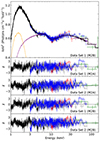 |
Fig. 3. Spectra (black for Insight-HXMT/LE, red for Insight-HXMT/ME, green for Insight-HXMT/HE, gray for NuSTAR/FPMA and blue for NuSTAR/FPMB), model components of M2B, and spectral residuals of M2A and M2B. The black solid line is the total model fitted to the data, and the yellow and purple dotted lines show the kerrbb2 and relxill spectral components, respectively. The models are plotted based on the best-fit parameters obtained from Insight-HXMT. |
Joint fitting parameters of Insight-HXMT and NuSTAR with M2 (constant*tbabs*(kerrbb2+relxill)).
4. Discussion
In this work, we perform a joint fitting of the simultaneous spectra of GRS 1716–249 observed by Insight-HXMT and NuSTAR. The data used are obtained during the softest phase of the outburst, where the disk component is most prominent and the inner edge of the disk is located at the ISCO (Bassi et al. 2019). Additionally, the presence of significant reflection features in the spectra allows us to measure the spin and inclination of the black hole, using a combined fitting method for the continuum and reflection components.
4.1. System parameters with updated distance
The fitting of the continuum is intrinsically linked to the distance, as altering the distance will impact the determination of the inner disk radius, consequently influencing the constraint on the spin. By fitting the spectra using M2 with varying distance parameters, we obtain distinct spin results (refer to Table 5). Notably, assuming a distance of 2.4 kpc, we obtain a near-extreme spin, aligning with the findings in Tao et al. (2019). However, assuming a distance of 6.9 kpc based on the recent works of Saikia et al. (2022) and Casares et al. (2023), resulted in a moderate spin of a* ∼ 0.46, implying that this source is not a rapidly rotating BH. This suggests that the spin was previously overestimated under the prior distance assumption. The disk inclination, even with varying distance assumptions, remains nearly constant around 43 − 47°, which is within the error margin of the orbital inclination of 61 ± 15° (with 68% confidence), as reported by Casares et al. (2023).
Fitting results of partial parameters with M2 by assuming different distances.
In the joint fitting of the continuum and reflection spectra, the distance measurement primarily affects the fitting of the continuum spectrum model (kerrbb2). Therefore, to investigate the impact of distance changes on the model, we plotted the best-fit M2 with its disk component Kerrbb2 and reflection component relxill at different distances (shown as solid lines in Fig. 4). The variation in distance did not result in significant changes in the total models, with differences of less than 2% in each energy band (see Fig. 4 bottom panel). Importantly, we found that the energy corresponding to the peak flux of the disk component ( ) did not show significant changes. Since the observed flux is fixed, an increase in distance leads to an increase in the accretion rate, as indicated by the parameter Ṁ in Table 5. According to accretion disk theory (Shakura & Sunyaev 1973), when other parameters remain constant, an increase in the accretion rate causes
  to shift towards higher energies, while a decrease in spin leads to an increase in Rin (=RISCO), resulting in a decrease in
  . Therefore, to maintain a constant
  , the model compensates for the increase in accretion rate due to larger distances by reducing the spin. This corresponds to the inverse correlation between a* and Ṁ shown in Figs. B.1–B.3.
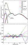 |
Fig. 4. Comparison diagram of different models. Top panel: Different models and their disk components and reflection components. Bottom panel: Ratio of each model relative to M2B. |
Furthermore, when other parameters remain constant, an increase in BH mass will cause  to shift towards lower energies. In this case, the model compensates for the mass increase by increasing the spin. Therefore, within the constraints of distance and mass provided by Casares et al. (2023), setting the lower limit (upper limit) of distance and the upper limit (lower limit) of mass yields the upper (lower) limit of the spin. When fixing the distance at 5.8 kpc and the BH mass at 9.6 M⊙ (M3; see Table A.1), we obtain a moderately high spin value of
  , with a goodness of fit of χ2/dof = 6416.4/6358 (see Fig. B.4 for the parameter probability distribution of dataset 1). When fixing the distance at 8 kpc and the BH mass at 4.4 M⊙ (M4; See Table A.1), we obtain a near non-rotating black hole with
  , with a goodness of fit of χ2/dof = 6499.9/6358. The red and green dashed lines in Fig. 4 represent M3 and M4. Therefore, considering the upper and lower limits of distance and mass provided by Casares et al. (2023), there will be a wider range of spin with a* < 0.78.
The above discussion indicates that the variation in the measured spin values with changes in distance and mass is a result of the degeneracy in the model. A similar phenomenon was observed when measuring the spins of LMC X–1 and Cyg X–1 using continuum spectra (Zdziarski et al. 2024). Their analysis shows that the disk components dominate the spectra, so the  derived from fitting matches the energy of the peak flux seen in the spectra (
 ). Increasing the hardening factor or convolving with Comptonization components outside the disk components will shift the
  towards higher energies. To maintain
  corresponding as closely as possible to
  , the remaining free parameters in the continuum spectrum, spin, and accretion rate, will decrease accordingly to counteract the effects of the hardening factor or Comptonization component.
Furthermore, the inconsistency in the iron abundance at different distances as shown in Table 5 (AFe> 9.3 for D = 2.4 and 3 kpc; AFe∼ 5 for D = 4–8 kpc) reflects not only the degeneracies among the parameters of the continuum model, but also a certain level of competition between the continuum and reflection components, particularly in the low energy band of ≲2 keV (García et al. 2018b; Tomsick et al. 2018). For instance, M2 with D = 2.4 and 3 kpc (as depicted in Fig. 4) exhibits a relatively higher proportion of disk components and a diminished reflection component compared to other models. The shape of the reflection spectrum in the low energy is significantly influenced by the configuration of the incident spectrum and the parameters of the disk as the reflector, leading to intertwined dependencies among various parameters in the overall model and rendering the parameter space exceptionally complicated. Zdziarski et al. (2024) reported local minimum iron abundance of AFe≲ 1 and global minimum values of AFe∼ 8 at Δχ2 ≈ −0.6 while fitting the spectra of LMC X-1 using continuum and reflection components (kerrbb2+reflkerr), thereby corroborating this point. Therefore, for obtaining more rational and precise parameters during spectral fitting, a comprehensive analysis of the entire parameter space is imperative to assess any biases that may potentially be introduced.
4.2. Further insights into spin measurements
Therefore, we attempted to replace kerrbb2 with diskbb, which only has two parameters, disk temperature, Tin, in units of keV and Norm, without considering the impact of distance, and re-conducted the spectral fitting (M5 = constant*tbabs*(diskbb+relxill); See Table A.1). The fitting results are shown in Table 6, which are very close to the fitting results of M1A. We obtained an extreme spin of a* ≳ 0.99, which is similar to the results obtained by Draghis et al. (2024) using the reflection component fitting method; that is, using the model diskbb combined with a reflection model. Furthermore, utilizing diskbb Norm ≈ 5000–6000 and i ≈ 48° of M5, and assuming a distance of D = 5.8–8 kpc, a hardening factor of fh = 1.3 (from M1A), and a boundary condition correction factor ζ = 0.412, we obtained the inner disk radius Rin≈ 35–53 km, using the formula  (Kubota et al. 1998). Assuming the source mass of 4.4–9.6 M⊙ (Casares et al. 2023), the gravitational radius Rg is about 6.5–14.3 km; thus, M5 yields Rin ≈ 2.4 − 8.2 Rg. By setting Rin = RISCO, the spin derived from the diskbb component is a* ∼ −0.72 − 0.88, which is inconsistent with the result of extreme spin obtained from the reflection model.
Joint fitting parameters of Insight-HXMT and NuSTAR with Tbabs*(diskbb+relxill).
Similarly to GRS 1716–249, when constraining the spin of some other sources, such as LMC X-3 (Draghis et al. 2024; Steiner et al. 2014), H 1743–322 (Draghis et al. 2023; Steiner et al. 2012), and MAXI J1820+070 (Draghis et al. 2023; Guan et al. 2021; Zhao et al. 2021), results obtained solely from the reflection component fitting method yield close to extreme spin values, while the continuum spectrum fitting method yields low spins of a* ≲ 0.3. The examples above demonstrate that when fitting the spectrum, using either the continuum or the reflection component fitting method separately resulted in different inner radii of the accretion disk, leading to different spin values and, hence, physically inconsistent results. The joint fitting method of the continuum and reflection components may help to avoid this issue by considering the jointly optimal parameter space during the fitting process.
5. Conclusion
In conclusion, we re-evaluated several key parameters of the black hole GRS 1716–249, utilizing simultaneous data from Insight-HXMT and NuSTAR. Through the application of a combined fitting method for the continuum and reflection components and the integration of updated distance and black hole mass, we found that the black hole has a moderate spin and a moderately inclined accretion disk. Given the source distance of 6.9 kpc and the black hole mass of 6.4 M⊙, we find that a* is  and i is
  , with a 90% confidence level. Taking into account the uncertainties in distance and black hole mass, the spin range extends with a*< 0.78.
The script can be found in https://github.com/NuSTAR/nustar-gen-utils/tree/3a603ca820a93c81414a298fd90d2e5a05f5e24a/notebooks
Version 2.0 of the relxill model is used in this work.
Acknowledgments
We thank the anonymous referee for useful comments that have allowed us to improved this manuscript. This work made use of data from the Insight-HXMT mission, a project funded by China National Space Administration (CNSA) and the Chinese Academy of Sciences (CAS). This work is supported by the National Key R&D Program of China (2021YFA0718500). We acknowledge funding support from the National Natural Science Foundation of China (NSFC) under grant Nos. 12122306, 12333007 and 12027803, the CAS Pioneer Hundred Talent Program Y8291130K2, the Strategic Priority Research Program of the Chinese Academy of Sciences under grant No. XDB0550300, the Scientific and technological innovation project of IHEP Y7515570U1 and the International Partnership Program of Chinese Academy of Sciences (Grant No.113111KYSB20190020) .
References
- Arnaud, K. A. 1996, ASP Conf. Ser., 101, 17 [Google Scholar]
- Ballet, J., Denis, M., Gilfanov, M., et al. 1993, IAU Circ., 5874, 1 [NASA ADS] [Google Scholar]
- Bassi, T., Del Santo, M., D’Aì, A., et al. 2019, MNRAS, 482, 1587 [NASA ADS] [CrossRef] [Google Scholar]
- Brown, G. E., & Bethe, H. A. 1994, ApJ, 423, 659 [NASA ADS] [CrossRef] [Google Scholar]
- Casares, J., Yanes-Rizo, I. V., Torres, M. A. P., et al. 2023, MNRAS, 526, 5209 [NASA ADS] [CrossRef] [Google Scholar]
- Chatterjee, K., Debnath, D., Chatterjee, D., et al. 2021, Ap&SS, 366, 63 [NASA ADS] [CrossRef] [Google Scholar]
- Corral-Santana, J. M., Casares, J., Muñoz-Darias, T., et al. 2016, A&A, 587, A61 [NASA ADS] [CrossRef] [EDP Sciences] [Google Scholar]
- Dauser, T., Garcia, J., Parker, M. L., Fabian, A. C., & Wilms, J. 2014, MNRAS, 444, L100 [Google Scholar]
- Davis, S. W., Blaes, O. M., Hubeny, I., & Turner, N. J. 2005, ApJ, 621, 372 [CrossRef] [Google Scholar]
- della Valle, M., Mirabel, I.F., & Rodriguez, L.F. 1994, A&A, 290, 803 [NASA ADS] [Google Scholar]
- Draghis, P. A., Miller, J. M., Zoghbi, A., et al. 2023, ApJ, 946, 19 [NASA ADS] [CrossRef] [Google Scholar]
- Draghis, P. A., Miller, J. M., Costantini, E., et al. 2024, ApJ, 969, 40 [NASA ADS] [CrossRef] [Google Scholar]
- Fabian, A. C., Rees, M. J., Stella, L., & White, N. E. 1989, MNRAS, 238, 729 [Google Scholar]
- García, J., Dauser, T., Lohfink, A., et al. 2014, ApJ, 782, 76 [Google Scholar]
- García, J. A., Steiner, J. F., McClintock, J. E., et al. 2015, ApJ, 813, 84 [Google Scholar]
- García, J. A., Steiner, J. F., Grinberg, V., et al. 2018a, ApJ, 864, 25 [CrossRef] [Google Scholar]
- García, J. A., Kallman, T. R., Bautista, M., et al. 2018b, ASP Conf. Ser., 515, 282 [NASA ADS] [Google Scholar]
- Guan, J., Tao, L., Qu, J. L., et al. 2021, MNRAS, 504, 2168 [NASA ADS] [CrossRef] [Google Scholar]
- Guo, C.-C., Liao, J.-Y., Zhang, S., et al. 2020, J. High Energy Astrophys., 27, 44 [NASA ADS] [CrossRef] [Google Scholar]
- Harmon, B. A., Fishman, G. J., Paciesas, W. S., & Zhang, S. N. 1993, IAU Circ., 5900, 1 [NASA ADS] [Google Scholar]
- Kubota, A., Tanaka, Y., Makishima, K., et al. 1998, PASJ, 50, 667 [NASA ADS] [CrossRef] [Google Scholar]
- Li, L.-X., Zimmerman, E. R., Narayan, R., & McClintock, J. E. 2005, ApJS, 157, 335 [NASA ADS] [CrossRef] [Google Scholar]
- Liao, J.-Y., Zhang, S., Lu, X.-F., et al. 2020a, J. High Energy Astrophys., 27, 14 [NASA ADS] [CrossRef] [Google Scholar]
- Liao, J.-Y., Zhang, S., Chen, Y., et al. 2020b, J. High Energy Astrophys., 27, 24 [NASA ADS] [CrossRef] [Google Scholar]
- Masetti, N., Bianchini, A., Bonibaker, J., & della Valle, M., & Vio, R., 1996, A&A, 314, 123 [NASA ADS] [Google Scholar]
- McClintock, J. E., Shafee, R., Narayan, R., et al. 2006, ApJ, 652, 518 [NASA ADS] [CrossRef] [Google Scholar]
- McClintock, J. E., Narayan, R., Davis, S. W., et al. 2011, Classical Quantum Gravity, 28 [Google Scholar]
- McClintock, J. E., Narayan, R., & Steiner, J. F. 2014, Space Sci. Rev., 183, 295 [NASA ADS] [CrossRef] [Google Scholar]
- Miller, J. M. 2007, ARA&A, 45, 441 [NASA ADS] [CrossRef] [Google Scholar]
- Negoro, H., Masumitsu, T., Kawase, T., et al. 2016, ATel, 9876, 1 [NASA ADS] [Google Scholar]
- Novikov, I. D., & Thorne, K. S. 1973, Black Holes (Les Astres Occlus), 343 [Google Scholar]
- Özel, F., Psaltis, D., Narayan, R., & McClintock, J. E. 2010, ApJ, 725, 1918 [CrossRef] [Google Scholar]
- Parker, M. L., Tomsick, J. A., Miller, J. M., et al. 2015, ApJ, 808, 9 [NASA ADS] [CrossRef] [Google Scholar]
- Remillard, R. A., & McClintock, J. E. 2006, ARA&A, 44, 49 [Google Scholar]
- Reynolds, C. S. 2021, ARA&A, 59, 117 [NASA ADS] [CrossRef] [Google Scholar]
- Reynolds, C. S., & Nowak, M. A. 2003, Phys. Rep., 377, 389 [NASA ADS] [CrossRef] [Google Scholar]
- Reynolds, C. S., & Fabian, A. C. 2008, ApJ, 675, 1048 [NASA ADS] [CrossRef] [Google Scholar]
- Saikia, P., Russell, D. M., Baglio, M. C., et al. 2022, ApJ, 932, 38 [NASA ADS] [CrossRef] [Google Scholar]
- Salvesen, G., & Miller, J. M. 2021, MNRAS, 500, 3640 [Google Scholar]
- Shakura, N. I., & Sunyaev, R. A. 1973, A&A, 24, 337 [NASA ADS] [Google Scholar]
- Steiner, J. F., Reis, R. C., McClintock, J. E., et al. 2011, MNRAS, 416, 941 [CrossRef] [Google Scholar]
- Steiner, J. F., McClintock, J. E., & Reid, M. J. 2012, ApJ, 745, L7 [NASA ADS] [CrossRef] [Google Scholar]
- Steiner, J. F., McClintock, J. E., Orosz, J. A., et al. 2014, ApJ, 793, L29 [NASA ADS] [CrossRef] [Google Scholar]
- Tao, L., Tomsick, J. A., Qu, J., et al. 2019, ApJ, 887, 184 [NASA ADS] [CrossRef] [Google Scholar]
- Tomsick, J. A., Parker, M. L., García, J. A., et al. 2018, ApJ, 855, 3 [NASA ADS] [CrossRef] [Google Scholar]
- Verner, D. A., Ferland, G. J., Korista, K. T., & Yakovlev, D. G. 1996, ApJ, 465, 487 [Google Scholar]
- Walton, D. J., Mooley, K., King, A. L., et al. 2017, ApJ, 839, 110 [NASA ADS] [CrossRef] [Google Scholar]
- Wilms, J., Allen, A., & McCray, R. 2000, ApJ, 542, 914 [Google Scholar]
- Zdziarski, A. A., Banerjee, S., Chand, S., et al. 2024, ApJ, 962, 101 [NASA ADS] [CrossRef] [Google Scholar]
- Zhang, S. N., Cui, W., & Chen, W. 1997, ApJ, 482, L155 [NASA ADS] [CrossRef] [Google Scholar]
- Zhao, X., Gou, L., Dong, Y., et al. 2021, ApJ, 916, 108 [NASA ADS] [CrossRef] [Google Scholar]
Appendix A: Definitions of the range of models
Range of models and the setting of the black hole mass (M) and distance (D) parameters in the disk components.
Appendix B: Probability distributions of the parameters from dataset 1
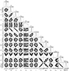 |
Fig. B.1. Probability distributions of the parameters for M1B obtained from dataset 1 through MCMC. |
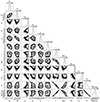 |
Fig. B.2. Probability distributions of the parameters for M2A obtained from dataset 1 through MCMC. |
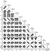 |
Fig. B.3. Probability distributions of the parameters for M2B obtained from dataset 1 through MCMC. |
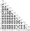 |
Fig. B.4. Probability distributions of the parameters for M3 obtained from dataset 1 through MCMC. |
All Tables
Joint fitting parameters of Insight-HXMT and NuSTAR with M1 (constant*tbabs*(kerrbb+relxill)).
Joint fitting parameters of Insight-HXMT and NuSTAR with M2 (constant*tbabs*(kerrbb2+relxill)).
Joint fitting parameters of Insight-HXMT and NuSTAR with Tbabs*(diskbb+relxill).
Range of models and the setting of the black hole mass (M) and distance (D) parameters in the disk components.
All Figures
|
Fig. 1. MAXI/GSC light-curve (2–20 keV) of GRS 1716–249. The solid red vertical line represents the simultaneous Insight-HXMT and NuSTAR observations used in this work. |
| In the text | |
|
Fig. 2. Light curves of Insight-HXMT/LE (top pannel) and NuSTAR/FPMA (bottom panel). The black dashed vertical line represents the division point for both datasets. |
| In the text | |
|
Fig. 3. Spectra (black for Insight-HXMT/LE, red for Insight-HXMT/ME, green for Insight-HXMT/HE, gray for NuSTAR/FPMA and blue for NuSTAR/FPMB), model components of M2B, and spectral residuals of M2A and M2B. The black solid line is the total model fitted to the data, and the yellow and purple dotted lines show the kerrbb2 and relxill spectral components, respectively. The models are plotted based on the best-fit parameters obtained from Insight-HXMT. |
| In the text | |
|
Fig. 4. Comparison diagram of different models. Top panel: Different models and their disk components and reflection components. Bottom panel: Ratio of each model relative to M2B. |
| In the text | |
|
Fig. B.1. Probability distributions of the parameters for M1B obtained from dataset 1 through MCMC. |
| In the text | |
|
Fig. B.2. Probability distributions of the parameters for M2A obtained from dataset 1 through MCMC. |
| In the text | |
|
Fig. B.3. Probability distributions of the parameters for M2B obtained from dataset 1 through MCMC. |
| In the text | |
|
Fig. B.4. Probability distributions of the parameters for M3 obtained from dataset 1 through MCMC. |
| In the text | |
Current usage metrics show cumulative count of Article Views (full-text article views including HTML views, PDF and ePub downloads, according to the available data) and Abstracts Views on Vision4Press platform.
Data correspond to usage on the plateform after 2015. The current usage metrics is available 48-96 hours after online publication and is updated daily on week days.
Initial download of the metrics may take a while.