| Issue |
A&A
Volume 691, November 2024
|
|
|---|---|---|
| Article Number | A92 | |
| Number of page(s) | 12 | |
| Section | Astrophysical processes | |
| DOI | https://doi.org/10.1051/0004-6361/202451260 | |
| Published online | 31 October 2024 | |
Broadband X-ray spectral and timing properties of the accreting millisecond X-ray pulsar IGR J17498−2921 during the 2023 outburst
1
Key Laboratory of Stars and Interstellar Medium, Xiangtan University, Xiangtan, 411105 Hunan, P.R. China
2
SRON-Netherlands Institute for Space Research, Sorbonnelaan 2, 3584 CA Utrecht, The Netherlands
3
International Space Science Institute (ISSI), Hallerstrasse 6, 3012 Bern, Switzerland
4
Physikalisches Institut, University of Bern, Sidlerstrasse 5, 3012 Bern, Switzerland
5
Department of Physics and Astronomy, FI-20014 University of Turku, Finland
6
Space Research Institute of the Russian Academy of Sciences, Profsoyuznaya str. 84/32, 117997 Moscow, Russia
7
Department of Astronomy, School of Physics, Peking University, Beijing 100871, People’s Republic of China
8
Kavli Institute for Astronomy and Astrophysics, Peking University, Beijing 100871, People’s Republic of China
9
Key Laboratory of Particle Astrophysics, Institute of High Energy Physics, Chinese Academy of Sciences, 19B Yuquan Road, Beijing 100049, China
⋆ Corresponding author; This email address is being protected from spambots. You need JavaScript enabled to view it.
Received:
26
June
2024
Accepted:
9
September
2024
Abstract
We report on the broadband spectral and timing properties of the accreting millisecond X-ray pulsar IGR J17498−2921 during its April 2023 outburst. We used data from NICER (1–10 keV), NuSTAR (3–79 keV), Insight-HXMT (2–150 keV), and INTEGRAL (30–150 keV). We detected significant 401 Hz pulsations across the 0.5–150 keV band. The pulse fraction increases from ∼2% at 1 keV to ∼13% at 66 keV. We detected five type-I X-ray bursts, including three photospheric radius expansion bursts, with a rise time of ∼2 s and an exponential decay time of ∼5 s. The recurrence time is ∼9.1 h, which can be explained by unstable thermonuclear burning of hydrogen-deficient material on the neutron star surface. The quasi-simultaneous 1–150 keV broadband spectra from NICER, NuSTAR and INTEGRAL can be aptly fitted by an absorbed reflection model, relxillCp, and a Gaussian line of instrumental origin. The Comptonized emission from the hot corona is characterized by a photon index Γ of ∼1.8 and an electron temperature kTe of ∼40 keV. We obtained a low inclination angle i ∼ 34°. The accretion disk shows properties of strong ionization, log(ξ/erg cm s−1)∼4.5, over-solar abundance, AFe ∼ 7.7, and high density, log(ne/cm−3)∼19.5. However, a lower disk density with normal abundance and ionization could also be possible. Based on the inner disk radius of Rin = 1.67RISCO and the long-term spin-down rate of −3.1(2)×10−15 Hz s−1, we were able to constrain the magnetic field of IGR J17498−2921 to the range of (0.9 − 2.4)×108 G.
Key words: radiation mechanisms: non-thermal / stars: neutron / pulsars: individual: IGR J17498-2921 / X-rays: general
© The Authors 2024
 Open Access article, published by EDP Sciences, under the terms of the Creative Commons Attribution License (https://creativecommons.org/licenses/by/4.0), which permits unrestricted use, distribution, and reproduction in any medium, provided the original work is properly cited.
This article is published in open access under the Subscribe to Open model. This email address is being protected from spambots. You need JavaScript enabled to view it. to support open access publication.
1. Introduction
Accreting millisecond X-ray pulsars (AMXPs) are binary systems hosting a rapidly rotating, old (∼Gyr) neutron star (NS) with a relatively weak magnetic field of 108 − 9 G and a low-mass companion. Overall, AMXPs are identified based on their coherent X-ray pulsations at spin frequencies higher than ∼100 Hz during X-ray outbursts (see Campana & Di Salvo 2018; Di Salvo & Sanna 2022; Papitto et al. 2020; Patruno & Watts 2021, for reviews). On average, about one new AMXP is discovered per year since the first confirmed source SAX J1808.4–3658. Among the most recent, we note MAXI J1816–195 (Bult et al. 2022; Li et al. 2023) and MAXI J1957+032 (Sanna et al. 2022) in 2022 and SRGA J144459.2–604207 (Ray et al. 2024; Li et al. 2024; Ng et al. 2024; Molkov et al. 2024) in 2024. In addition, a few outbursts from the known AMXP sample may also be observed each year.
IGR J17498−2921 was discovered by INTEGRAL during its 2011 outburst, and confirmed as an AMXP with the spin frequency of ∼401 Hz, orbital period of 3.8 hr, and projected semi-major axis, aX sin i/c ≈ 0.365 lt-s (Papitto et al. 2011). The source position using Chandra X-ray observation was determined at  and
and  with an uncertainty of
  at a 90% confidence level (Chakrabarty et al. 2011). The coherent pulsations have been detected up to 65 keV with an energy-independent pulsed fraction of 6–7%. The pulse profiles are well described by a sine wave and the soft lags of ∼ − 60 μs have been detected which saturated near 10 keV (Falanga et al. 2012).
During the 2011 outburst of IGR J17498−2921, type-I X-ray bursts were discovered, including one photospheric radius expansion (PRE) burst observed by RXTE (Linares et al. 2011; Falanga et al. 2012). The distance to the source was estimated at 8 kpc. From the burst profiles and recurrence times one could conclude that they were powered by the unstable burning of pure helium or the material with the CNO metallicity up to twice solar abundance. The burst oscillation signal around its spin frequency has been detected mainly during the cooling tail (Chakraborty & Bhattacharyya 2012).
In this work, we study the NICER, NuSTAR, Insight-HXMT, and INTEGRAL observations of IGR J17498−2921 during its 2023 outburst. The data analysis and the outburst profile are introduced in Sects. 2 and 3, respectively. The spectral evolution during NICER observations and the broadband spectra are reported in Sect. 4. We investigate the timing properties of IGR J17498−2921 in Sect. 5. The X-ray burst properties are presented in Sect. 6. We discuss all the results in Sect. 7.
2. Observations
After twelve years in quiescence, IGR J17498−2921 showed new activity cycle as was first noticed by Grebenev et al. (2023) using INTEGRAL data on 2023 April 13–15. NICER, Insight-HXMT, and NuSTAR had carried out dedicated follow-up observations, covering the main epoch of the outburst (Sanna et al. 2023). We collected data from IGR J17498−2921 observed by these instruments as well as those from INTEGRAL during its April 2023 outburst.
2.1. INTEGRAL
In this work, we used mainly data from the coded mask soft gamma-ray imager IBIS/ISGRI (Ubertini et al. 2003; Lebrun et al. 2003) aboard INTEGRAL (Winkler et al. 2003) at energies from 20 to 150 keV. For ISGRI, the data were extracted for all pointings with a source position offset  . The data reduction was carried out using the standard Offline Science Analysis (OSA) version 11 distributed by the INTEGRAL Science Data Center (Courvoisier et al. 2003).
INTEGRAL Galactic centre ToO observations – targeting Sgr A* and GX 5−1 – during satellite revolution (Rev.) 2628 on 2023 April 13–15 (MJD 60047.181–60049.378) showed renewed activity of AMXP IGR J17498−2921 (Grebenev et al. 2023) in IBIS-ISGRI data. A zoom-in on Rev. 2628 revealed that IGR J17498−2921 reached already a 8.3σ detection in the 20–60 keV band during the 25.2 ks ToO observation of Sgr A* performed at the beginning of Rev. 2628 on MJD 60047.181–60047.441. Since the onset of the outburst IGR J17498−2921 was in the INTEGRAL field of view during Galactic centre observations performed throughout revolutions 2628 (176.4 ks; 28.4σ), 2629 (73.8 ks; 27.8σ), 2630 (119.4 ks; 29.1σ), 2632 (50 ks; 10.5σ), and 2634 (100 ks; 16.2σ), covering the period of April 13–30, 2023 (MJD 60047.181–60064.39). The significance values were quoted for the 20–60 keV band. We also analyzed the pre-outburst 2023 Galactic centre observations performed during Revs. 2623–2625 (311.2 ks), clearly indicating that IGR J17498−2921 was off. For the spectral analysis, we extracted a (outburst averaged) combined spectrum from the mosaic of Revs. 2628–2630/2632/2634 observations, when the source displayed a relatively flat outburst profile, with the source flux being about 30 mCrab (see Fig. 1).
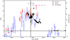 |
Fig. 1. Light curves of IGR J17498−2921 from NICER (black dot, 0.5–10 keV, in units of cnt s−1), MAXI/GSC (blue open circle, 2.0–6.0 keV), and INTEGRAL/ISGRI (red open square, 20–60 keV) during its 2023 outburst. The MAXI rate is in units of ph cm−2 s−1 multiplied by 560 to overlap with the NICER data. The scale of the 20–60 keV ISGRI light curve is shown along the right vertical axis and is given in units of mCrab. The grey area presents the epoch of NuSTAR observations. The black arrows on the upper center mark the start time of five type I X-ray bursts with burst number. The horizontal dashed line shows the background level. The vertical purple lines present the start time of Insight-HXMT observations. The count rates of the three Insight-HXMT instruments were polluted by several nearby (Galactic center) sources; therefore, they are not included here. |
2.2. NICER
NICER provides non-imaging detectors with a field of view (FOV) of 30 arcmin2 and an absolute timing accuracy of 100 ns. About one week after the detection of the 2023 outburst of IGR J17498−2921 by INTEGRAL, NICER carried out follow-up observations starting on 2023 April 20 (MJD 60054). The last observation ended on 2023 July 8 (MJD 60134), when the source was returned to a quiescent state. In total, 46 NICER observations have become available, including Obs IDs 6203770101∼6203770105 and 6560010101∼6560010141. The total exposure time is 130 ks, including 81 ks in the outburst (i.e., the first 18 observations from April 20 to May 3) and 49 ks in quiescence (i.e., the last 28 observations from May 15 to July 8).
The NICER data were processed by using HEASOFT V6.31 and the NICER Data Analysis Software (NICERDAS) version 10. The standard filtering criteria were applied, including an angular offset of the source ANG_DIST lower than  , as well as an Earth limb elevation angle and bright Earth limb angle larger than 20° and 30°, respectively, an undershoot rate of underonly_range = 0–500, an overshoot rate of overonly_range = 0–30, and a NICER location outside the South Atlantic Anomaly. We extracted 1 s binned light curves in the 0.5–10 and 12–15 keV bands using the command nicerl3-lc. Time intervals showing flaring background in 12–15 keV light curves were discarded from further analysis.
We identified one type I X-ray burst in Obs. Id. 6560010101 (see Sect. 6). The spectra were generated using nicerl3-spect tool, while the associated ancillary response files (ARFs), response matrix files (RMFs), and 3C50 background spectra (Remillard et al. 2022) were produced simultaneously.
In the timing analysis, we used a multi-mission serving barycentering tool adopting the JPL DE405 Solar System ephemeris, written in IDL and developed at SRON, which is equivalent and compatible with HEASOFT tool barycorr. To estimate the background-corrected pulsed emission properties (see Sect. 5.3), we used NICER data collected during Obs. Ids. 6560010114–6560010119 (2023 May 15–20; MJD 60079.9–60084.4; 9.389 ks GTI time)1 as a background reference sample when the source was in a well-established Off state (see Fig. 1).
2.3. NuSTAR
NuSTAR has observed IGR J17498−2921 on 2023 April 23 for a total exposure time of 44.6 ks (Obs. ID 90901317002, MJD 60057.44–60058.48). The event files from FPMA and FPMB were cleaned using the NuSTAR pipeline tool nupipeline.
The source light curves were extracted from a circle region with a radius of 100″ centered on the source location using nuproducts. The count rate from NuSTAR maintained a constant level of ∼19 cnt s−1 in the 3–79 keV band, except for two type I X-ray bursts that showed up during the NuSTAR observation. We excluded these two X-ray bursts in producing the source spectra, response, and ancillary response files to perform joint spectral fitting with NICER spectra (see Sect. 4.2). The background spectra were obtained from a source free circular region with a radius of 100″ centered at  . We also generated time-resolved burst spectra for the two X-ray bursts with the option usrgtifile applied in the command nuproducts.
For the timing studies, we used barycentered events adopting the JPL DE405 Solar System ephemeris and applying fine-clock-correction file #169, from a circular region with a radius of 90″ centered on the Chandra X-ray location (Chakrabarty et al. 2011) of IGR J17498−2921 as a source sample. To obtain background corrected quantities like pulsed fraction (see Sect. 5.3), we used a source free circular region (located on the same chip as our target) with a radius of 90″ centered at  as a background reference sample.
2.4. Insight-HXMT
The Insight-HXMT (Insight Hard X-ray Modulation Telescope, Zhang et al. 2020) has three slat-collimated and non-imaging telescopes, the Low Energy X-ray telescope (LE, 1–12 keV; Chen et al. 2020), the Medium Energy X-ray telescope (ME, 5–35 keV; Cao et al. 2020), and the High Energy X-ray telescope (HE, 20–350 keV; Liu et al. 2020), which have the capabilities of broadband X-ray timing and spectroscopy. The FOV of Insight-HXMT is approximately 6 ° ×6°. The absolute timing accuracy of Insight-HXMT was verified from the alignment of the pulse profiles in the AMXP MAXI J1816–195; namely, within 14 μs between Insight-HXMT/ME and NICER, and 0.9 ± 13.9 μs between Insight-HXMT ME and HE, in the same energy bands (Li et al. 2023). Insight-HXMT has carried out twelve ToO observations (PI, Z. Li, Obs. ID P0504093001–P0504093012) between April 23 and May 7, 2023. We analyzed the data using the Insight-HXMT Data Analysis Software (HXMTDAS V2.05). The LE, ME, and HE data were calibrated by using the scripts lepical, mepical, and hepical, respectively. For each instrument, the good time intervals (GTIs) were individually obtained from the scripts legtigen, megtigen, and hegtigen, resulting in the exposure time of 13.6, 89.6, and 70.3 ks from LE, ME, and HE, respectively.
We obtained background-subtracted light curves from LE, ME and HE in 2–10, 10–35 and 27–250 keV, respectively. Two type I X-ray bursts were observed, the first from Obs ID P050409300302 with LE and ME data available, while the second from Obs ID P050409300402 only from ME data. After ignoring these X-ray bursts, the count rates remained at constant levels of 51.6, 15.7, and 33.5 cnt s−1 for LE, ME and HE, respectively. However, the NICER light curve showed a reduction in count-rate of at least a factor of two during the Insight-HXMT observations. Therefore, due to its large FOV the Insight-HXMT LE, ME, and HE light curves were strongly affected by the nearby bright sources; for instance, the persistent black hole candidate 1E 1740.7–2942 located at  from the source position. Therefore, we did not perform a joint spectral fitting using the Insight-HXMT LE/ME/HE data (see Sect. 4). The nearby bright sources did not exhibit pulsation signatures around 401 Hz, and their emissions only contributed to a higher (statistically flat) background level in the pulsation studies.
We used the timing data from Insight-HXMT ME and HE, barycentered using the tool hxbary with the JPL DE405 Solar System ephemeris, to study the X-ray pulsation of IGR J17498−2921. For the X-ray bursts, we extract the pre-burst spectra and the time-resolved burst spectra via the tools lespecgen and mespecgen, and their response matrix files are generated from lerspgen and merspgen, for LE and ME, respectively. In Sect. 6, we offer details on the X-ray burst studies.
3. Outburst profile
In Fig. 1, we show the outburst profile of IGR J17498−2921 during the 2023 outburst, which includes the observations from NICER (0.5–10 keV), MAXI (2.0–6.0 keV), INTEGRAL/ISGRI (20–60 keV). The Insight-HXMT light curves are not presented in Fig. 1 due to the pollution of nearby sources, but the start time of Insight-HXMT observations are marked as vertical purple lines. The observations of the outburst rise were poorly covered. By interpolating the INTEGRAL/ISGRI light curve, the onset of the outburst was determined around MJD 60040. At the same time, the MAXI rate was still consistent with the background, indicating a hard spectral state at the beginning of the outburst. The source reached its peak within 5 days. In the next ∼10 days, from the NICER 0.5–10 keV light curves, IGR J17498−2921 had experienced complicated fluctuations, which exhibited three main peaks on MJD 60055.1, 60058.4, and 60060.8 with the rate of ∼90, ∼85, and ∼110 cnt s−1, respectively. Starting after the third peak, the count rate decreased slowly to quiescent. During this process, a reflare in the later stage of the outburst appeared on MJD 60066.5 with a peak rate of ∼60 cnt s−1. From the MAXI data, the source returned to the quiescent state before MJD 60074, namely, the outburst lasted around one month. During the quiescent state, the NICER count rate was consistent with the background level without distinct reflares. The onset time of five type I X-ray bursts are labeled as vertical arrows in Fig. 1.
4. Spectral analysis
We used XSPEC version 12.13.0c (Arnaud 1996) to fit the persistent spectra from IGR J17498−2921. The Tübingen-Boulder absorption model (tbabs), with abundances from Wilms et al. (2000), was applied to account for the interstellar medium absorption. There are several quasi-simultaneous observations between NICER and Insight-HXMT. The joint NICER and Insight-HXMT spectral fitting revealed that the Insight-HXMT fluxes were 3–5 times higher than the NICER flux. Similar to the count rate from Insight-HXMT, the spectra reconfirm that a nearby source contributed more than IGR J17498−2921 in the Insight-HXMT data. Therefore, we only fit NICER spectra for the whole outburst in Sect. 4.1, and performed the joint NICER, NuSTAR, and INTEGRAL spectral fitting, as described in Sect. 4.2. The uncertainties for all the parameters are quoted at the 1σ confidence level.
4.1. NICER spectra
We fit the NICER spectra in between MJD 60054.3–60067.3. After MJD 60067.3, no NICER spectra were available until the source returned to the quiescent state. Below 1 keV, the NICER spectra showed substantial excess possibly due to instrumental origin; therefore, we focused on the 1–10 keV energy range. We fit the continuum with a thermal Comptonized component, nthcomp, modified by photoelectric absorption modeled by tbabs. The residuals also showed an emission feature at 1.6–1.7 keV from the instrument. We added a Gaussian component to account for it. The whole model is tbabs×(Gaussian+nthcomp). The parameters include the hydrogen column density, NH, for Tbabs, the line energy, width, and normalization for Gaussian, the asymptotic power-law photon index, Γ, the electron temperature, kTe, the seed photon temperature, kTbb, the type of the seed photons, and the normalization for nthcomp. We set the type for the seed photons to a blackbody distribution. The bolometric flux was estimated via cflux in 1–250 keV. The uncertainties were obtained from the command error.
The best-fitting parameters are shown in Fig. 2. The bolometric flux showed fluctuations between (0.92 − 1.35)×10−9 erg s−1 cm−2 for the first ∼8 days, then slowly decayed to ∼5 × 10⁻¹⁰ erg s−1 cm−2 within one reflare in the next ∼7 days. We found increasing and then decreasing variations of the hydrogen column density, NH ∼ (2.4 − 2.9)×1022 cm−2, and the power-law photon index, Γ ∼ 1.6 − 1.8, as well as opposite trends of the electron temperature, kTe ∼ 2.9 − 9.4 keV, and the seed photon temperature, kTBB ∼ 0.25 − 0.46 keV, with a quasi-periodical timescale of 4 ∼ 5 days.
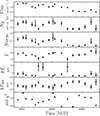 |
Fig. 2. Best-fitting parameters of NICER spectra using the model tbabs*(Gaussian+nthcomp). |
4.2. Broadband spectral fitting
We performed a quasi-simultaneously joint spectral fitting between NICER, NuSTAR and INTEGRAL for IGR J17498−2921, covering the energy range of 1–150 keV. The spectra were collected between MJD 60057.51–60057.53 for NICER Obs. ID 6203770103, MJD 60057.44–60058.48 for NuSTAR. We also produced the average INTEGRAL/IBIS-ISGRI spectrum during MJD 60047.16–60064.39 to guarantee a high signal-to-noise ratio (S/N). We introduced a multiplication factor for each instrument to account for the cross-calibration uncertainties and possible flux variations. The factor was fixed at unity for NuSTAR/FPMA and set free for other instruments.
We first attempted to fit the joint spectra using the model as mentioned above tbabs*(nthcomp+gaussian). The model was not able to fully explain the broadband spectra with χν2 ≈ 4.0 for 565 degrees of freedom (d.o.f.). We also tried the thermal Comptonization model, compps (Poutanen & Svensson 1996), in the slab geometry, which was applied to its 2011 outburst (Falanga et al. 2012), but the fit was also very poor, χν2 ≈ 3.0 for 563 d.o.f. (see also Falanga et al. 2005b,a, 2008, 2011, 2012; De Falco et al. 2017b,a; Li et al. 2018; Kuiper et al. 2020; Li et al. 2021, 2023). We note that the residuals show a reflection feature. Therefore, we replaced nthcomp with the relativistic reflection model relxillCp, where the incident spectrum is modeled by an nthcomp Comptonization continuum (see Ludlam 2024, for more details). The free parameters of the model are as follows: the inclination of the system, i, the inner radius of the disc, Rin, in units of the inner-most stable circular orbit (ISCO, RISCO), the power law index of the incident spectrum, Γ, the electron temperature in the corona, kTe, the logarithm of the disk ionization, log ξ, the iron abundance normalized to the Sun, AFe, the density of the disk in logarithmic units, log ne, and the reflection fraction, frefl.. We fixed the inner and outer emissivity indices, q1 and q2 (both at 3), the break radius between these two emissivity indices and the outer disk radius, Rout = Rbreak = 1000Rg, where Rg = GMNS/c2 is the gravitational radius, and G and c are the gravitational constant and the speed of light, respectively. Assuming the NS mass and radius of 1.4M⊙ and 10 km, respectively, for IGR J17498−2921 spinning at 401 Hz, we obtained the dimensionless spin parameter a = 0.188, which was also fixed. The model fit the spectra acceptably with χν2 ≈ 1.12 for 560 d.o.f.. We tried to add an extra thermal component, bbodyrad from the NS surface, or diskbb from the accretion disk, to the model, however, the fit did not improve significantly, namely, Δχ2 < 3 with two more free parameters. Therefore, we propose that no significant thermal emissions from the disc or NS surface are found in the spectra. Moreover, no apparent features appeared in the residuals (see Fig. 3).
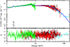 |
Fig. 3. Joint spectral fitting of NICER, NuSTAR and INTEGRAL/IBIS-ISGRI. The spectra were observed during MJD 60057.51–60057.53 for NICER (green), MJD 60057.44–60058.48 for NuSTAR (red for FPMA and black for FPMB), and MJD 60047.4–60064.4 for INTEGRAL/IBIS (cyan). The black dashed line shows the Gaussian component at 1.7 keV, likely an instrumental feature. The blue solid line represents the best-fitting model tbabs×(Gaussian+relxillcp). |
We applied the Goodman–Weare Markov chain Monte Carlo (MCMC) algorithm to investigate the best-fit parameters further to produce contour plots (Goodman & Weare 2010). We adopted 100 walkers and a chain length of 5 × 10⁶ to calculate the marginal posterior distributions. The first 105 steps were set as burn-in length and discarded. The contours are presented in Fig. 4, which were produced by using the procedure corner.py (Foreman-Mackey 2016). The 1σ confidence levels of the best-fit parameters from MCMC are listed in Table 1. The unabsorbed bolometric flux is (1.45 ± 0.01)×10−9 erg s−1 cm−2 in 1–250 keV, which is larger than the result solely from the NICER spectrum reported in Sect. 4.1 because of the use of different datasets and models. The NH is (3.15 ± 0.03)×1022 cm−2, slightly higher than the results from the NICER spectra, but consistent with the value reported by Bozzo et al. (2011). All the multiplication factors are close to unity, suggesting proper calibration between all instruments and no strong variability during the quasi-simultaneous observations. The obtained values characterize the accretion disk of strong ionization, over-solar abundance, and high density. The Comptonized emission associated with a hot corona is characterized by the photon index of 1.78 ± 0.01 and the electron temperature of kTe = 39 ± 4 keV, implying a hard spectral state. The inclination angle of the accretion disk is 34 ± 4 deg, in agreement with the absence of dips or eclipses in the light curves. From the relation RISCO = 6GMNS/c2[1 − a(2/3)3/2] (Miller et al. 1998), the inner disk radius Rin = 1.67RISCO corresponds to  km, suggesting that the accretion disk is located rather closed to the NS surface for a typical radius of 10 km. On the other hand, the obtained inner disk radius set an upper limit of the NS radius (see Ludlam 2024, and references therein), which is consistent with most NS equations of state (see Burgio et al. 2021, and references therein).
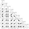 |
Fig. 4. Posterior distributions of the fitted parameters obtained by MCMC simulations. The parameters of the Gaussian component and the normalization of relxillCp are not shown here. |
Best-fit spectral parameters of the NICER/NuSTAR/INTEGRAL data for IGR J17498−2921 for the model constant×tbabs×(gaussian+relxillCp).
We explored the possibility of lower solar abundance by fixing AFe at two times solar abundance. However, the model fit the spectra poorly with χν2 = 1.59 for 561 d.o.f.. Adding an extra blackbody component with a temperature of 1.6 ± 0.1 keV and normalization of  , the best-fitting results improved to χν2 = 1.40 for 559 d.o.f., which was also worse than the model described above. We noticed that only the inner disk radius,
  , and the electron temperature, kTe = 30 ± 8 keV, changed significantly, but still comparable with the results in Table 1. Therefore, we conclude that the current model with lower solar abundance does not adequately fit the broadband spectra.
5. Timing analysis
An accurate timing analysis offers a wide variety of important information on the neutron star (binary) system, including its accretion disk (during outburst), and its orbital- and spin evolution, as well as the physical processes involved in the generation of the pulsed emission.
The first step in the timing analysis is the conversion of the on-board event arrival time expressed in MJD for the Terrestial Time system (TDT or TT) to the solar-system barycenter arrival time for the TDB time system. For this process, we used: (a) the JPL DE405 solar system ephemeris; (b) the instantaneous spacecraft location with respect to the Earth’s center, and (c) the (currently) most accurate source location of IGR J17498−2921 as obtained by Chakrabarty et al. (2011) using Chandra soft X-ray data (see Table 2). In the event selection procedure, we ignored time intervals during which type I X-ray bursts occurred or high-background rates were encountered (see Sect. 2.2).
Orbital and spin parameters of IGR J17498−2921 as derived in this work from a 4D optimization scheme using NICER 1.5–10 keV data.
5.1. NICER, NuSTAR, Insight-HXMT, and INTEGRAL
Because NICER monitoring observations during the 2023 outburst provided the most uniform and sensitive exposure to IGR J17498−2921 we used this set to construct an accurate timing model of the binary milli-second pulsar. The pulsed signal strength, evaluated through the bin-free Z1, 22-test statistics (Buccheri et al. 1983), is a function of four parameters assuming a constant spin rate of the neutron star and a circular orbit (eccentricity e ≡ 0). We employed a 4D optimization scheme based on a downhill SIMPLEX algorithm by iteratively improving the Z2-statistics with respect to four parameters: the spin frequency, ν, the projected semi-major axis of the neutron star, ax sin i, the orbital period, Porb, and the time-of-ascending node, Tasc (see e.g., De Falco et al. 2017b; Li et al. 2021, for earlier (lower) dimensional versions of the method)2
As start values for this optimization procedure (not a blind search), we used the system parameters of IGR J17498−2921 as derived for the previous 2011 outburst (see e.g., Falanga et al. 2012; Papitto et al. 2011, and references therein), except for the Tasc parameter, which we adapted for current epoch using the 2011 orbital period value. The optimized values and their 1σ uncertainties, shown in Table 2, are based on the first eighteen NICER observations covering MJD 60054.301–60067.520 and totaling 69.425 ks of (good time/screened) exposure collected during the ON phase of the 2023 outburst. With the accurate spin- and orbital parameters given in Table 2, we can calculate (for any high-energy instrument used in this work) the (spin) pulse-phase of each selected event, taking into account the orbital motion of the pulsar. Thus, we can construct pulse-phase distributions for various energy bands within the instrument bandpass.
A compilation of pulse-phase distributions (outburst integrated) for different high-energy instruments in different energy bands is shown in Fig. 5. The pulsed emission is significantly detected from ∼0.5 keV (NICER) up to ∼150 keV (Insight-HXMT/HE) with a 60–150 keV pulse significance of ∼3.5σ (see Fig. 5m). The pulse-shape is approximately sinusoidal and remarkably stable as a function of energy.
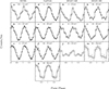 |
Fig. 5. 0.5–150 keV broadband pulse-phase distributions of IGR J17498−2921 observed by NICER (panels a–c, 0.5–10 keV), NuSTAR (panels d–g, 3–60 keV), and Insight-HXMT (panels h–j, 5–35 keV for ME; panels k–m, 20–150 keV for HE). Two cycles are shown to improve clarity. The error bars represent 1σ errors. The morphology is almost unchanged with energy. All profiles reach their maximum near phase ∼0.1. |
Also INTEGRAL-IBIS-ISGRI (not shown in Fig. 5) has detected pulsed emission from IGR J17498−2921 in a combination of data from observations taken during INTEGRAL revolutions 2630, 2632, and 2634 (MJD 60053.282-60063.761) with at the highest energies a 55–90 keV pulsed emission significance of ∼3.5σ. Remarkably, no pulsed emission (20–60 keV) was detected at the early stage of the outburst during the revolutions 2628 (discovery revolution; see Grebenev et al. 2023) and 2629 from MJD 60047.181–60050.708 when the source flux was rising to its (first) maximum (see Fig. 1, and also Papitto et al. 2020).
5.2. Variability of the pulsed emission: signal strength and pulse arrival
In correcting the barycentered NICER event arrival times for the orbital motion induced delays, we studied the pulsed emission strength across the course of the outburst using the Z12-test statistics as a proxy for the S/N (Buccheri et al. 1983). We identified a ∼2 d duration episode on MJD 60060.03–60061.92 with 8.594 ks of GTI exposure exhibiting strongly suppressed pulsed emission with a Z12 signal strength value of 4.7σ. This episode coincides with the general maximum in the NICER lightcurve shown in Fig. 1. NICER observations performed just before (MJD 60059.015–60059.975; 8.884 ks) and after (MJD 60062.225–60062.944; 4.508 ks) this episode showed pulsed-signal strength of 20.6σ and 30.7σ, respectively. Apparently, the pulsed signal was quenched during the period showing maximum accretion rate. It is interesting to note that during the NICER observation (MJD 60059.015–60059.975) preceding the "quenched" episode the spin-frequency was about 3.4(5)×10−6 (∼7σ) larger than the outburst averaged value shown in Table 2, likely indicating a short duration spin-up period just before reaching maximum luminosity. Near the end of the outburst at MJD 60066.098–60067.520, a similar, but less pronounced (5.6σ in 2.871 ks) episode of quenched pulsed emission is found in NICER data; this is also coincident with a (local) maximum in the outburst light curve.
Next, we investigated the stability of the (binary motion corrected) pulse-arrival times by applying a time-of-arrival (ToA) analysis (see e.g. Kuiper & Hermsen 2009, for more details). This method assumes a stable invariant pulse shape of IGR J17498−2921 across the outburst in the correlation process with a high-statistics template. This method was applied to Insight-HXMT HE 20–60 keV data and yielded seven ToA measurements across MJD 60057–600713 that were scattered slightly around the (outburst averaged spin-frequency) model prediction. Minimizing the Insight-HXMT HE ToA phase residuals yielded a spin frequency of ν = 400.990 185 94(3)Hz with a best fit root-mean-square (RMS) of 0.023 in phase units (≡57.2 μs in time domain), consistent at a 2σ level with the (outburst averaged) value (given in Table 2).
The ToA method applied to fifteen 1.5–10 keV NICER measurements yielded a RMS of 0.092 in phase units (≡228 μs), which is sufficiently small to guarantee phase coherence across the outburst, but the scatter is too large to be explained by statistical fluctuations. Apparently, systematics due to accretion induced processes play an important role in the soft X-ray regime, and result in rather large fluctuations in the pulse-arrival times.
5.3. Pulsed fraction and time lag
From the pulse-phase distributions in different (measured) energy bands (see e.g., Fig. 5), we can deduce some important intrinsic emission properties of the pulsed emission providing clues to the emission mechanism. Focusing now on NICER and NuSTAR, since we can perform reliable background subtraction for these instruments (contrary to the Insight-HXMT instruments given the weakness of the outburst); thus, we can estimate the intrinsic (background subtracted) pulsed fraction as a function of energy band. The measured pulse-phase distributions (for a selected energy interval) can be described in terms of a truncated Fourier series,
![Mathematical equation: $$ \begin{aligned} F(\phi ) = A_0 + \sum _{k=1}^2 A_k \ \cos [2\pi \ k (\phi -\phi _k)], \end{aligned} $$](/articles/aa/full_html/2024/11/aa51260-24/aa51260-24-eq17.gif) (1)
(1)
where A0 is a constant, A1 and A2 are the amplitudes, ϕ1 and ϕ2 are the phase angles in units of radians/2π, of the fundamental and the first overtone, respectively. We can determine the global minimum for each energy band, and from this along with the total number of background subtracted source counts the intrinsic pulsed fraction. The result of this procedure is shown in the left panel of Fig. 6. It is clear from this plot that the intrinsic pulsed fraction steadily increases from ∼2% to ∼13% going from soft X-rays at 0.5 keV (NICER; open circles) up to hard X-rays at 66 keV (NuSTAR; filled diamonds). This pronounced trend was not visible in the 2011 outburst data, being consistent with constant (cf. Fig. 7 of Falanga et al. 2012) and having poor statistical quality in the hard X-ray regime above ∼20 keV.
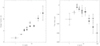 |
Fig. 6. Background subtracted pulsed fraction as a function of (measured) energy using (outburst averaged) NICER data (open circles) across the 0.5–10 keV band and NuSTAR data (filled diamonds) across the 3–66 keV range (left). The pulsed fraction clearly increases as a function of energy going from ∼2% near 1 keV to ∼13% at the 34–66 keV band. The time delay (in μs) relative to the NICER 3–4 keV band showing NICER (0.5–10 keV; open circles), NuSTAR (3–66 keV; filled diamonds), Insight-HXMT/ME (6–18 keV; filled circles) and Insight-HXMT/HE (18–130 keV; filled triangles) measurements (right). Events with energies above 4 keV systematically arrive earlier with an increasing trend as a function of energy than those from the reference 3–4 keV band. Also, the same is seen for (NICER) events from the soft band with energies below 3 keV (not properly accessible during the 2011 outburst). |
In this work, we have also determined the time lag as a function of energy with respect to a chosen reference energy band by applying a cross-correlation method (cf. Fig. 5 of Falanga et al. 2012). For this purpose, we used data from NICER, NuSTAR and also Insight-HXMT-ME/HE, because background subtraction is not required to obtain this quantity. The results using NICER 3–4 keV band as reference interval in the cross-correlation procedure are shown in the right panel of Fig. 6. Events having energies above 4 keV arrive earlier than the events from the 3–4 keV reference band in a decreasing way the higher the energy. The trend above ∼20 keV was not visible in the 2011 outburst data because of poor statistical quality. Events having energies below 3 keV (an interval that could not be studied before) also arrive earlier than the reference band.
Thanks to the detection of broadband pulse emissions from IGR J17498−2921, the observed time lag is unique compared with other AMXPs. For most AMXPs, the time lag is constant below ∼2–3 keV, and monotonically increasing with energy (the soft-energy pulsed photons lag behind the hard-energy ones) and saturating at about 6–20 keV (see e.g. Gierliński & Poutanen 2005; Falanga et al. 2011). The behaviors of time lag have been explained by the two-component model, that is, the soft blackbody component from a hot spot on the NS surface, and the hard Comptonized component from the up-scattering of the seed photons from hot spot by the accretion flow (Poutanen & Gierliński 2003; Gierliński & Poutanen 2005; Ibragimov & Poutanen 2009). The soft pulsation is dominated by the blackbody component, which vanishes above the saturated energy, that is, the higher saturated energy corresponding to a stronger contribution of the blackbody component in the total flux or higher blackbody temperature (Falanga et al. 2011). However, we do not observe the saturated energy till 100 keV in IGR J17498−2921. Therefore, the hard and soft time lags observed in IGR J17498−2921 cannot be explained by this model. We note that the Comptonized component may have different patterns at different energy ranges.
6. Type-I X-ray bursts
From 1-s binned light curves, we identified five type I X-ray bursts, one from NICER (#1), two from NuSTAR (#2 and #3), and two from Insight-HXMT (#4 and #5). The burst light curves plotted in Fig. 7 all have similar profiles. For burst #5, only ME data are available. The burst rise time is defined as the interval between the first point when the flux exceeds that of the persistent emission by 5%, t5%, and the point when the count rate reaches 95% of that in the first peak, t95%. For each burst, we applied a linear interpolation to the light curve to determine t5% and t95%. The uncertainties in the rise time are estimated from the standard deviation of the peak rate of the light curve. All bursts showed a fast rise time of ∼2 s. Bursts #4 and #5 exhibited two peaks in the LE and ME data, and other bursts had only one peak. The flux from all bursts decreased exponentially to the pre-burst level. We searched for the burst oscillation in the frequency range of 396–406 Hz by applying Z12 statistic (Buccheri et al. 1983). The selected energy ranges are 0.5–10 keV for the NICER burst, 3–20 keV for two NuSTAR bursts, and 5–20 keV for two Insight-HXMT ME bursts. No significant oscillation signal was detected.
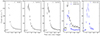 |
Fig. 7. Light curves of five X-ray bursts from IGR J17498−2921 detected by NICER (burst #1), NuSTAR (#2 and #3), and Insight-HXMT (#4 and #5). The trigger time of each burst is listed in the fourth column of Table 3. |
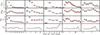 |
Fig. 8. Evolution of the spectral parameters of five X-ray bursts. Bursts are shown from left to right, in the same order as Fig. 7. |
The time-resolved spectra were extracted with an exposure time of 1–8 s, which ensured that the spectra had sufficient counts for a spectral fitting and would not miss the PRE burst features. We fit the burst spectra with an absorbed blackbody model, while the pre-burst spectra were regarded as background and assumed unchanged during bursts. We fixed the hydrogen column density, NH, at the values obtained in Sect. 4.1. The free parameters are the temperature, kTBB, and the normalization, K = Rph2/D10 kpc2, of the blackbody component. Most burst spectra were well fitted yielding χν2 of ∼1.0. We identified three PRE bursts from the time-resolved spectroscopy, namely, the first burst from NuSTAR and two bursts from Insight-HXMT. Assuming a distance of 8 kpc the radii of the photosphere expanded to 13.5 ± 0.3, 11.3 ± 0.7 and  km, with corresponding temperatures of 1.9 ± 0.1, 2.0 ± 0.1, and 2.2 ± 0.2 keV, for bursts #2, #4, and #5, respectively. The peak fluxes of all bursts are around (4.0 ± 0.5)×10−8 erg s−1 cm−2, which are lower than the brightest PRE burst reported by Falanga et al. (2012).
We fit the exponential decay of the bursts with the function F(t) = F0exp(−t/τ), where τ is the decay time, and found that all bursts had decay times close to 5 s. Next, the burst fluence was derived using the relation fb = Fpeakτ. The bursts’ short rise and decay times of our 2023 sample are consistent with those from the sample of the 2011 outburst, which were powered by unstable burning of hydrogen-deficient material. The properties of the 2023 outburst bursts, the start time, the rise time, the peak flux, the persistent flux, the decay time τ, and the burst fluence, are listed in Table 3.
IGR J17498−2921 burst properties for the 2023 outburst sample.
We calculated the burst recurrence times and obtained 50.1, 9.1, 37.7, and 27.5 hrs starting from the burst onset time. The pair of two NuSTAR bursts had the shortest recurrence time. We tentatively considered this to be the true recurrence time (i.e., assuming that no X-ray burst(s) were missed between these two bursts) which is shorter than the recurrence time of ∼16–18 hr found during the 2011 outburst (Falanga et al. 2012). The other recurrence times were 5.5, 4, and 3 times longer, indicating that some bursts could have been missed due to the data gaps.
The burst persistent fluxes were obtained from interpolating the flux reported in Sect. 4.1. All uncertainties were assigned as their typical values. The X-ray bursts were triggered during the outburst with the persistent flux in the range of (0.97 − 1.34)×10−9 erg s−1 cm−2. Assuming a distance of 8 kpc, the persistent flux corresponds to (0.74 − 1.03)×1037 erg s−1, or (2.0 − 2.7)%LEdd by using the empirical value of LEdd = 3.8 × 1038 erg s−1 (Kuulkers et al. 2003). The local accretion rate per unit area is calculated from the relation  , namely,
  , assuming the mass, MNS = 1.4M⊙, and radius, RNS = 10 km, of NS, and, thus, the gravitational redshift 1 + z = 1.31. From the observed burst fluences, the total burst released energies are Eb = 4πd2fb = (1.1 − 2.0)×1039 erg. We estimated the burst ignition depth via
  , where the nuclear energy generated for pure helium is Qnuc ≈ 1.31 MeV nucleon−1 for X = 0 (Goodwin et al. 2019). We obtained yign = (0.96 − 1.66)×108 g cm−2. Once the ignition depth was known, we calculated the recurrence time between bursts by using the equation Δtrec = (yign/̇m)(1 + z). The predicted recurrence time is (6.4 − 11.0) h, consistent with the observed values.
7. Discussion and summary
In this work, we study the X-ray pulsations, time-resolved and broadband spectra, and X-ray burst properties of the AMXP IGR J17498−2921 during its 2023 outburst. Five type I X-ray bursts have been detected, including three PRE bursts. These X-ray bursts exhibited similar profiles, with the rise time of ∼2 s, exponential decay time of ∼5 s, and a peak flux of around 4 × 10⁻⁸ erg s−1 cm−2. The peak fluxes of the PRE bursts are lower than that from the brightest burst observed by RXTE (Falanga et al. 2012). We measured a recurrence time of 9.1 h, shorter than the values, ∼16–18 h, observed during its 2011 outburst at a similar persistent flux. These properties can be well explained by the unstable burning of hydrogen-deficient material on the NS surface in IGR J17498−2921.
7.1. Broadband spectra
We analyzed the spectra observed from NICER, NuSTAR, Insight-HXMT and INTEGRAL IBIS-ISGRI, covering the 1–150 keV energy range. The NICER spectra in 1–10 keV can be well fitted with an absorbed nthcomp plus Gaussian model with NH ∼ (2.−2.9)×1022 cm−2, a power-law photon index Γ of ∼1.6–1.8, an electron temperature kTe of ∼2.9–9.4 keV, and a seed photon temperature kTBB of ∼0.25–0.46 keV. The bolometric flux reached its peak around 1.35 × 10⁻⁹ erg s−1 cm−2 in ∼2–3 d, similar to its 2011 outburst and also to other AMXPs. However, the source showed fluctuations in the next 10 d in both the soft and hard X-ray bands, which is peculiar, considering that a smooth decay is typically observed for most of the AMXP outbursts (Falanga et al. 2005b; Kuiper et al. 2020; Li et al. 2023). During the decay stage, a reflare appeared.
Marino et al. (2019) calculated the long-term average luminosity of IGR J17498−2921, assuming an orbital evolution driven by conservative mass transfer, by considering two possible mechanisms: gravitational radiation (GR) and magnetic braking (MB). They determined that the average luminosity was 1.8 × 1035 erg s−1 for the GR-only case and 3.7 × 1035 erg s−1 for the GR+MB case. However, the observed average X-ray luminosity before the 2023 outburst was significantly lower, at 0.61 × 1033 erg s−1, which is far below the theoretically predicted values. As a result, they suggested that non-conservative mass transfer likely occurred during the 2011 outburst of IGR J17498−2921. The 2023 outburst profile was close to that of 2011. Adding an extra outburst, the observed average luminosity over the last 20 years has doubled, but it remains below the predictions. Therefore, the 2023 outburst of IGR J174982921 likely involved non-conservative mass transfer as well.
The joint quasi-simultaneous NICER, NuSTAR, and INTEGRAL IBIS-ISGRI spectra in the energy range of 1–150 keV are well described by a self-consistent reflection model, relxillCp, with a Gaussian line, modified by interstellar absorption. The unabsorbed bolometric flux, Fbol, of the broadband spectrum was (1.45 ± 0.01)×10−9 erg s−1 cm−2, corresponding to ∼3%LEdd when assuming a source distance of 8 kpc. We can characterize the accretion flow properties by a photon index of 1.78 ± 0.01 and an electron temperature of kTe = 39 ± 4 keV. The inclination angle of the binary system is 34 ± 3 deg. We found a high reflection fraction of frefl = 5.2−0.7+1.0, which means most of the photons interacted with the surrounding disk first rather than emitted directly to the observer. It is self-consistent with our first measurement of the inner disk radius  for IGR J17498−2921. The broadband spectral fitting shows the properties of the accretion disk as a strong ionization,
  , over-solar abundance,
  , and a high density, log(ne/cm−3) = 19.5−0.5+0.3. There are several X-ray binaries showing over-solar abundance in the spectra, which can be alternatively explained by a reflection model with a higher disk density (see e.g., Ludlam et al. 2017, 2018, 2019; Tomsick et al. 2018; Connors et al. 2021; Liu et al. 2023). In the case of IGR J17498−2921, we note that AFe and log ξ present significant negative covariances with log ne in Fig. 4. It is not surprising because the ionization parameter ξ is related to the accretion density ne via ξ = 4πFx/ne, where Fx is the total illuminating flux. For the persistent luminosity around a few percent of the Eddington limit, the disk density can reach up to ∼1022 cm−3 (Jiang et al. 2019). The upper limit of log ne in the current relxillCp model is 20. Therefore, a larger disk density with smaller ionization and solar abundance may also be possible. We also found that the important parameters, Rin and i, weakly depend on the disk density. Thus, a higher ne does not affect our measurements of these two parameters. From the pulsar mass function, f(MNS, MC, i) = MC3sin3i/(MNS + MC)2 ≈ 2 × 10⁻³ M⊙, we can calculate the companion star mass MC=(0.32–0.41)M⊙ for MNS∼1.4–2M⊙ if the accretion disk is aligned with the binary orbit.
7.2. Orbital period refinement
Comparing the orbital solutions obtained for the 2011 and 2023 outbursts, we can improve the orbital period Porb. The integer number of orbital cycles between  MJD and
  MJD from current work and Falanga et al. (2012), respectively, amounts Ncyc= int
  . In turn, assuming that the orbital period between two outbursts is unchanged, we can refine the orbital period to
  s, where the error is mainly from the uncertainty in
  given in Table 2.
Constraints on the upper and lower limits of Ṗorb are also possible, even though a direct measurement is impossible with only two Tasc measurements. Using the equation from Burderi et al. (2009) or Riggio et al. (2011), Ṗorb is expressed as
 (2)
(2)
where ΔTasc(Ncyc) = Tasc, 2023 − (Tasc, 2011 + Ncyc × Porb) is the difference between the predicted and measured time of the ascending node in 2023. If we adopt the upper and lower limits of the orbital period, Porb = 13835.619(1) s, and ΔPorb = 0.001 s measured by Papitto et al. (2011), we obtain a result of Ṗorb of ( − 3, +8)×10−12 s s−1 at a 1σ confidence level.
7.3. Stellar magnetic field and long-term spin evolution
If we assume that the inner accretion disk is truncated at the magnetospheric (Alfvén) radius, the magnetic dipole moment can be expressed as (Psaltis & Lamb 1999; Ibragimov & Poutanen 2009),
 (3)
(3)
where μ26 = μ/1026 G cm3, η is the accretion efficiency, the conversion factor, kA, and the angular anisotropy factor, fang, are set to unity, the distance, D, to the source is 8 kpc, and the bolometric flux and the inner disk radius from Sect. 4.2 are used. If we adopt η ∼ 0.1 − 0.2, the NS mass, MNS ∼ 1.4 − 2M⊙, and radius, RNS ∼ ∼ 10 − 15 km, a distance uncertainty of 0.8 kpc, and the inner disk radius,  km, the magnetic dipole moment is μ26 ∼ 0.6 − 2.4. This estimation converts to the NS magnetic field of (0.2 − 2.4)×108 G.
The timing solution reported by Papitto et al. (2011) is ν = 400.99018734(1) Hz,  and Porb = 13835.619(1) s at the reference epoch T0 = 55786.124 MJD during the 2011 outburst. Considering the 2011 outburst lasting between MJD 55786.1–55826.4, we obtain a spin frequency of 400.99018712(7) at the end of the 2011 outburst. If we assume that the pulsar was spinning down at a constant rate during the quiescent state, which lasted from the end of the 2011 outburst to the beginning of the 2023 outburst, then we can compute an averaged long-term spin-down rate of
  ; here, the error is calculated by propagating the uncertainties in spin frequencies. If the average spin-down rate during the quiescent state is caused by (rotating) magnetic dipole emission, the magnetic dipole moment is (Spitkovsky 2006):
 (4)
(4)
where θ is the angle between the rotation and magnetic axes, I45 is the NS moment of inertia in units of 1045 g cm2, the spin frequency, ν2 = ν/100 Hz, and the spin frequency derivative is  . If we adopt the same range of NS radius as Eq. (3) and sin2θ ∼ 0 − 1, we have the magnetic dipole moment μ26 ∼ 1.6 − 2.2, corresponding to a magnetic field strength of (0.9 − 4.4)×108 G. The deduced magnetic field is consistent with the value calculated from Eq. (3). If we combine the results from Eqs. (3) and (4), then we obtain a constraint on the magnetic field of (0.9 − 2.4)×108 G, which is compatible with those of other AMXPs (see e.g., Hartman et al. 2008; Patruno et al. 2009; Patruno 2010; Hartman et al. 2009, 2011; Papitto et al. 2011; Li et al. 2023) and the samples provided in Mukherjee et al. (2015).
Observations performed before the ‘optical light leak’ period that commenced on May 22, 2023 between 13:00–14:00 UTC.
The downhill SIMPLEX method is an optimization algorithm to find the global minimum of a multi-parameter function. The statement in the second paragraph of Sect. 5 in De Falco et al. (2017b) indicates the need to find the global minimum of −Z12-test statistic and so, to obtain the maximum of the Z12 distribution.
Note: Insight-HXMT HE data showed pulsed emission up to MJD 60071.389 i.e., beyond the last NICER observation ending at MJD 60067.325 during the ON phase of the outburst.
Acknowledgments
We appreciate the valuable comments from the referee, which has contributed to improving our manuscript. This work was supported by the Major Science and Technology Program of Xinjiang Uygur Autonomous Region (No. 2022A03013-3), the National Natural Science Foundation of China (12103042, 12273030, 12173103, U1938107), and Minobrnauki grant 075-15-2024-647 (JP). This research has made use of data obtained from the High Energy Astrophysics Science Archive Research Center (HEASARC), provided by NASA’s Goddard Space Flight Center, and also from the HXMT mission, a project funded by the China National Space Administration (CNSA) and the Chinese Academy of Sciences (CAS).
References
- Arnaud, K. A. 1996, ASP Conf. Ser., 101, 17 [Google Scholar]
- Bozzo, E., Ferrigno, C., Papitto, A., & Gibaud, L. 2011, ATel., 3555, 1 [NASA ADS] [Google Scholar]
- Buccheri, R., Bennett, K., Bignami, G. F., et al. 1983, A&A, 128, 245 [NASA ADS] [Google Scholar]
- Bult, P., Altamirano, D., Arzoumanian, Z., et al. 2022, ApJ, 935, L32 [NASA ADS] [CrossRef] [Google Scholar]
- Burderi, L., Riggio, A., di Salvo, T., et al. 2009, A&A, 496, L17 [NASA ADS] [CrossRef] [EDP Sciences] [Google Scholar]
- Burgio, G. F., Schulze, H. J., Vidaña, I., & Wei, J. B. 2021, Prog. Part. Nucl. Phys., 120, 103879 [CrossRef] [Google Scholar]
- Campana, S., & Di Salvo, T. 2018, ASSL, 457, 149 [NASA ADS] [Google Scholar]
- Cao, X., Jiang, W., Meng, B., et al. 2020, Sci. Chin. Phys. Mech. Astron., 63, 249504D [CrossRef] [Google Scholar]
- Chakraborty, M., & Bhattacharyya, S. 2012, MNRAS, 422, 2351 [NASA ADS] [CrossRef] [Google Scholar]
- Chakrabarty, D., Markwardt, C. B., Linares, M., & Jonker, P. G. 2011, ATel., 3606, 1 [NASA ADS] [Google Scholar]
- Chen, Y., Cui, W., Li, W., et al. 2020, Sci. Chin. Phys. Mech. Astron., 63, 249505D [NASA ADS] [CrossRef] [Google Scholar]
- Connors, R. M. T., García, J. A., Tomsick, J., et al. 2021, ApJ, 909, 146 [NASA ADS] [CrossRef] [Google Scholar]
- Courvoisier, T. J. L., Walter, R., Beckmann, V., et al. 2003, A&A, 411, L53 [NASA ADS] [CrossRef] [EDP Sciences] [Google Scholar]
- De Falco, V., Kuiper, L., Bozzo, E., et al. 2017a, A&A, 603, A16 [NASA ADS] [CrossRef] [EDP Sciences] [Google Scholar]
- De Falco, V., Kuiper, L., Bozzo, E., et al. 2017b, A&A, 599, A88 [NASA ADS] [CrossRef] [EDP Sciences] [Google Scholar]
- Di Salvo, T., & Sanna, A. 2022, ASSL, 465, 87 [NASA ADS] [Google Scholar]
- Falanga, M., Bonnet-Bidaud, J. M., Poutanen, J., et al. 2005a, A&A, 436, 647 [NASA ADS] [CrossRef] [EDP Sciences] [Google Scholar]
- Falanga, M., Kuiper, L., Poutanen, J., et al. 2005b, A&A, 444, 15 [NASA ADS] [CrossRef] [EDP Sciences] [Google Scholar]
- Falanga, M., Chenevez, J., Cumming, A., et al. 2008, A&A, 484, 43 [NASA ADS] [CrossRef] [EDP Sciences] [Google Scholar]
- Falanga, M., Kuiper, L., Poutanen, J., et al. 2011, A&A, 529, A68 [NASA ADS] [CrossRef] [EDP Sciences] [Google Scholar]
- Falanga, M., Kuiper, L., Poutanen, J., et al. 2012, A&A, 545, A26 [NASA ADS] [CrossRef] [EDP Sciences] [Google Scholar]
- Foreman-Mackey, D. 2016, J. Open Source Software, 1, 24 [NASA ADS] [CrossRef] [Google Scholar]
- Gierliński, M., & Poutanen, J. 2005, MNRAS, 359, 1261 [Google Scholar]
- Goodman, J., & Weare, J. 2010, Commun. Appl. Math. Comput. Sci., 5, 65 [Google Scholar]
- Goodwin, A. J., Heger, A., & Galloway, D. K. 2019, ApJ, 870, 64 [NASA ADS] [CrossRef] [Google Scholar]
- Grebenev, S. A., Bryksin, S. S., & Sunyaev, R. A. 2023, ATel., 15996, 1 [NASA ADS] [Google Scholar]
- Hartman, J. M., Patruno, A., Chakrabarty, D., et al. 2008, ApJ, 675, 1468 [NASA ADS] [CrossRef] [Google Scholar]
- Hartman, J. M., Patruno, A., Chakrabarty, D., et al. 2009, ApJ, 702, 1673 [NASA ADS] [CrossRef] [Google Scholar]
- Hartman, J. M., Galloway, D. K., & Chakrabarty, D. 2011, ApJ, 726, 26 [NASA ADS] [CrossRef] [Google Scholar]
- Ibragimov, A., & Poutanen, J. 2009, MNRAS, 400, 492 [CrossRef] [Google Scholar]
- Jiang, J., Fabian, A. C., Wang, J., et al. 2019, MNRAS, 484, 1972 [NASA ADS] [CrossRef] [Google Scholar]
- Kuiper, L., & Hermsen, W. 2009, A&A, 501, 1031 [NASA ADS] [CrossRef] [EDP Sciences] [Google Scholar]
- Kuiper, L., Tsygankov, S. S., Falanga, M., et al. 2020, A&A, 641, A37 [NASA ADS] [CrossRef] [EDP Sciences] [Google Scholar]
- Kuulkers, E., den Hartog, P. R., in’t Zand, J. J. M., et al. 2003, A&A, 399, 663 [NASA ADS] [CrossRef] [EDP Sciences] [Google Scholar]
- Lebrun, F., Leray, J. P., Lavocat, P., et al. 2003, A&A, 411, L141 [NASA ADS] [CrossRef] [EDP Sciences] [Google Scholar]
- Li, Z., De Falco, V., Falanga, M., et al. 2018, A&A, 620, A114 [NASA ADS] [CrossRef] [EDP Sciences] [Google Scholar]
- Li, Z. S., Kuiper, L., Falanga, M., et al. 2021, A&A, 649, A76 [NASA ADS] [CrossRef] [EDP Sciences] [Google Scholar]
- Li, Z., Kuiper, L., Ge, M., et al. 2023, ApJ, 958, 177 [CrossRef] [Google Scholar]
- Li, Z., Kuiper, L., Falanga, M., et al. 2024, ATel., 16548, 1 [NASA ADS] [Google Scholar]
- Linares, M., Altamirano, D., Watts, A., et al. 2011, ATel., 3568, 1 [NASA ADS] [Google Scholar]
- Liu, C., Zhang, Y., Li, X., et al. 2020, Sci. China Phys. Mech. Astron., 63, 249503 [NASA ADS] [CrossRef] [Google Scholar]
- Liu, H., Jiang, J., Zhang, Z., et al. 2023, ApJ, 951, 145 [NASA ADS] [CrossRef] [Google Scholar]
- Ludlam, R. M. 2024, Ap&SS, 369, 16 [NASA ADS] [CrossRef] [Google Scholar]
- Ludlam, R. M., Miller, J. M., Bachetti, M., et al. 2017, ApJ, 836, 140 [CrossRef] [Google Scholar]
- Ludlam, R. M., Miller, J. M., Arzoumanian, Z., et al. 2018, ApJ, 858, L5 [Google Scholar]
- Ludlam, R. M., Miller, J. M., Barret, D., et al. 2019, ApJ, 873, 99 [Google Scholar]
- Marino, A., Di Salvo, T., Burderi, L., et al. 2019, A&A, 627, A125 [NASA ADS] [CrossRef] [EDP Sciences] [Google Scholar]
- Miller, M. C., Lamb, F. K., & Cook, G. B. 1998, ApJ, 509, 793 [NASA ADS] [CrossRef] [Google Scholar]
- Molkov, S. V., Lutovinov, A. A., Tsygankov, S. S., et al. 2024, A&A, 690, A353 [NASA ADS] [CrossRef] [EDP Sciences] [Google Scholar]
- Mukherjee, D., Bult, P., van der Klis, M., & Bhattacharya, D. 2015, MNRAS, 452, 3994 [NASA ADS] [CrossRef] [Google Scholar]
- Ng, M., Ray, P. S., Sanna, A., et al. 2024, ApJ, 968, L7 [NASA ADS] [CrossRef] [Google Scholar]
- Papitto, A., Bozzo, E., Ferrigno, C., et al. 2011, A&A, 535, L4 [NASA ADS] [CrossRef] [EDP Sciences] [Google Scholar]
- Papitto, A., Falanga, M., Hermsen, W., et al. 2020, New Astron. Rev., 91, 101544 [Google Scholar]
- Patruno, A. 2010, ApJ, 722, 909 [NASA ADS] [CrossRef] [Google Scholar]
- Patruno, A., & Watts, A. L. 2021, ASSL, 461, 143 [NASA ADS] [Google Scholar]
- Patruno, A., Altamirano, D., Hessels, J. W. T., et al. 2009, ApJ, 690, 1856 [NASA ADS] [CrossRef] [Google Scholar]
- Poutanen, J., & Gierliński, M. 2003, MNRAS, 343, 1301 [NASA ADS] [CrossRef] [Google Scholar]
- Poutanen, J., & Svensson, R. 1996, ApJ, 470, 249 [CrossRef] [Google Scholar]
- Psaltis, D., & Lamb, F. K. 1999, AAT, 18, 447 [NASA ADS] [Google Scholar]
- Ray, P. S., Strohmayer, T. E., Sanna, A., et al. 2024, ATel., 16480, 1 [NASA ADS] [Google Scholar]
- Remillard, R. A., Loewenstein, M., Steiner, J. F., et al. 2022, AJ, 163, 130 [NASA ADS] [CrossRef] [Google Scholar]
- Riggio, A., Burderi, L., di Salvo, T., et al. 2011, A&A, 531, A140 [NASA ADS] [CrossRef] [EDP Sciences] [Google Scholar]
- Sanna, A., Bult, P., Ng, M., et al. 2022, MNRAS, 516, L76 [NASA ADS] [CrossRef] [Google Scholar]
- Sanna, A., Ng, M., Guillot, S., et al. 2023, ATel., 15998, 1 [NASA ADS] [Google Scholar]
- Spitkovsky, A. 2006, ApJ, 648, L51 [Google Scholar]
- Tomsick, J. A., Parker, M. L., García, J. A., et al. 2018, ApJ, 855, 3 [NASA ADS] [CrossRef] [Google Scholar]
- Ubertini, P., Lebrun, F., Di Cocco, G., et al. 2003, A&A, 411, L131 [CrossRef] [EDP Sciences] [Google Scholar]
- Wilms, J., Allen, A., & McCray, R. 2000, ApJ, 542, 914 [Google Scholar]
- Winkler, C., Courvoisier, T. J.-L., Di Cocco, G., et al. 2003, A&A, 411, L1 [NASA ADS] [CrossRef] [EDP Sciences] [Google Scholar]
- Zhang, S.-N., Li, T., Lu, F., et al. 2020, Sci. China Phys. Mech. Astron., 63, 249502 [NASA ADS] [CrossRef] [Google Scholar]
All Tables
Best-fit spectral parameters of the NICER/NuSTAR/INTEGRAL data for IGR J17498−2921 for the model constant×tbabs×(gaussian+relxillCp).
Orbital and spin parameters of IGR J17498−2921 as derived in this work from a 4D optimization scheme using NICER 1.5–10 keV data.
All Figures
|
Fig. 1. Light curves of IGR J17498−2921 from NICER (black dot, 0.5–10 keV, in units of cnt s−1), MAXI/GSC (blue open circle, 2.0–6.0 keV), and INTEGRAL/ISGRI (red open square, 20–60 keV) during its 2023 outburst. The MAXI rate is in units of ph cm−2 s−1 multiplied by 560 to overlap with the NICER data. The scale of the 20–60 keV ISGRI light curve is shown along the right vertical axis and is given in units of mCrab. The grey area presents the epoch of NuSTAR observations. The black arrows on the upper center mark the start time of five type I X-ray bursts with burst number. The horizontal dashed line shows the background level. The vertical purple lines present the start time of Insight-HXMT observations. The count rates of the three Insight-HXMT instruments were polluted by several nearby (Galactic center) sources; therefore, they are not included here. |
| In the text | |
|
Fig. 2. Best-fitting parameters of NICER spectra using the model tbabs*(Gaussian+nthcomp). |
| In the text | |
|
Fig. 3. Joint spectral fitting of NICER, NuSTAR and INTEGRAL/IBIS-ISGRI. The spectra were observed during MJD 60057.51–60057.53 for NICER (green), MJD 60057.44–60058.48 for NuSTAR (red for FPMA and black for FPMB), and MJD 60047.4–60064.4 for INTEGRAL/IBIS (cyan). The black dashed line shows the Gaussian component at 1.7 keV, likely an instrumental feature. The blue solid line represents the best-fitting model tbabs×(Gaussian+relxillcp). |
| In the text | |
|
Fig. 4. Posterior distributions of the fitted parameters obtained by MCMC simulations. The parameters of the Gaussian component and the normalization of relxillCp are not shown here. |
| In the text | |
|
Fig. 5. 0.5–150 keV broadband pulse-phase distributions of IGR J17498−2921 observed by NICER (panels a–c, 0.5–10 keV), NuSTAR (panels d–g, 3–60 keV), and Insight-HXMT (panels h–j, 5–35 keV for ME; panels k–m, 20–150 keV for HE). Two cycles are shown to improve clarity. The error bars represent 1σ errors. The morphology is almost unchanged with energy. All profiles reach their maximum near phase ∼0.1. |
| In the text | |
|
Fig. 6. Background subtracted pulsed fraction as a function of (measured) energy using (outburst averaged) NICER data (open circles) across the 0.5–10 keV band and NuSTAR data (filled diamonds) across the 3–66 keV range (left). The pulsed fraction clearly increases as a function of energy going from ∼2% near 1 keV to ∼13% at the 34–66 keV band. The time delay (in μs) relative to the NICER 3–4 keV band showing NICER (0.5–10 keV; open circles), NuSTAR (3–66 keV; filled diamonds), Insight-HXMT/ME (6–18 keV; filled circles) and Insight-HXMT/HE (18–130 keV; filled triangles) measurements (right). Events with energies above 4 keV systematically arrive earlier with an increasing trend as a function of energy than those from the reference 3–4 keV band. Also, the same is seen for (NICER) events from the soft band with energies below 3 keV (not properly accessible during the 2011 outburst). |
| In the text | |
|
Fig. 7. Light curves of five X-ray bursts from IGR J17498−2921 detected by NICER (burst #1), NuSTAR (#2 and #3), and Insight-HXMT (#4 and #5). The trigger time of each burst is listed in the fourth column of Table 3. |
| In the text | |
|
Fig. 8. Evolution of the spectral parameters of five X-ray bursts. Bursts are shown from left to right, in the same order as Fig. 7. |
| In the text | |
Current usage metrics show cumulative count of Article Views (full-text article views including HTML views, PDF and ePub downloads, according to the available data) and Abstracts Views on Vision4Press platform.
Data correspond to usage on the plateform after 2015. The current usage metrics is available 48-96 hours after online publication and is updated daily on week days.
Initial download of the metrics may take a while.