| Issue |
A&A
Volume 690, October 2024
|
|
|---|---|---|
| Article Number | A210 | |
| Number of page(s) | 10 | |
| Section | Astronomical instrumentation | |
| DOI | https://doi.org/10.1051/0004-6361/202451389 | |
| Published online | 08 October 2024 | |
Accurate calibration spectra for precision radial velocities
Iodine absorption referenced by a laser frequency comb
1
Institut für Astrophysik und Geophysik, Georg-August-Universität,
Friedrich Hund Platz 1,
37077
Göttingen,
Germany
2
Institut für Quantenoptik, Leibniz Universität Hannover,
Welfengarten 1,
30167
Hannover,
Germany
★ Corresponding author; This email address is being protected from spambots. You need JavaScript enabled to view it.
Received:
5
July
2024
Accepted:
28
August
2024
Abstract
Astronomical spectrographs require calibration of their dispersion relation, for which external sources like hollow-cathode lamps or absorption-gas cells are useful. Laser frequency combs (LFCs) are often regarded as ideal calibrators because they provide the highest accuracy and dense sampling, but LFCs are facing operational challenges such as generating blue visual light or tunable offset frequencies. As an example of an external source, we aim to provide a precise and accurate frequency solution for the spectrum of molecular iodine absorption by referencing to an LFC that does not cover the same frequency range. We used a Fourier Transform Spectrometer (FTS) to produce a consistent frequency scale for the combined spectrum from an iodine absorption cell at 5200– 6200 Å and an LFC at 8200 Å. We used 17 807 comb lines to determine the FTS frequency offset and compared the calibrated iodine spectrum to a synthetic spectrum computed from a molecular potential model. In a single scan, the frequency offset was determined from the comb spectrum with an uncertainty of ∼1 cms−1. The distribution of comb line frequencies is consistent with no deviation from linearity. The iodine observation matches the model with an offset of smaller than the model uncertainties of ∼1 m s−1, which confirms that the FTS zero point is valid outside the range covered by the LFC, and that the frequencies of the iodine absorption model are accurate. We also report small systematic effects regarding the iodine model’s energy scale. We conclude that Fourier Transform Spectrometry can transfer LFC accuracy into frequency ranges not originally covered by the comb. This allows us to assign accurate frequency scales to the spectra of customized wavelength calibrators. The calibrators can be optimized for individual spectrograph designs regarding resolution and spectral bandwidth, and requirements on their long-term stability are relaxed because FTS monitoring can be performed during operation. This provides flexibility for the design and operation of calibration sources for high-precision Doppler experiments.
Key words: molecular data / instrumentation: spectrographs / methods: laboratory: molecular / techniques: radial velocities / reference systems
© The Authors 2024
 Open Access article, published by EDP Sciences, under the terms of the Creative Commons Attribution License (https://creativecommons.org/licenses/by/4.0), which permits unrestricted use, distribution, and reproduction in any medium, provided the original work is properly cited.
This article is published in open access under the Subscribe to Open model. This email address is being protected from spambots. You need JavaScript enabled to view it. to support open access publication.
1 Introduction
Precise and accurate measurements of frequencies (or wavelengths) in astronomical spectra enable a range of fundamental physical experiments. Frequency shifts occur through Doppler shifts allowing the measurement of velocities, which can be used, for example, to measure the mass of unseen extrasolar planets (Lindegren & Dravins 2003), stellar pulsations (Christensen-Dalsgaard 2004), and velocity fields in atmospheres of stars and planets (Asplund et al. 2000). Transition frequencies of spectral lines are determined and affected by fundamental constants like the fine structure constant and the proton/electron mass ratio (Dirac 1937; Webb et al. 1999; Martins et al. 2024), by gravitational redshift (Einstein 1911, 1916; Lindegren & Dravins 2003), and by the accelerated expansion of the Universe, which affects galaxy motion on very large scales (Liske et al. 2008). These and other experiments can be carried out if the frequency scale in spectra from astronomical objects can be accurately determined.
Astronomical spectroscopy is photon starved. Large telescopes are required to collect enough light from distant objects for astrophysical analysis, which is different from typical laboratory setups where the intensities of the investigated light can often be controlled. For precision Doppler measurements, high spectral resolution is favorable (Bouchy et al. 2001). Échelle spectrographs reach resolutions of R = λ/Δλ = 105 at efficiencies on the order of 10%. For comparison, a Fourier Transform Spectrometer (FTS) can operate at higher resolution and provides a number of advantages regarding frequency calibration, but delivers an efficiency that is several orders of magnitude lower than in astronomical spectrographs (see, e.g., Hajian et al. 2007).
In grating (échelle) spectrographs, light is collected in individual detector pixels that are at minimum several hundred m s−1 wide and are not strictly evenly spaced (Wilken et al. 2010). This poses a fundamental problem to frequency calibration because, in principle, each individual pixel requires calibration through external information. Furthermore, astronomical spectroscopy often requires a relatively large bandwidth – for example one octave – because information is collected simultaneously from many individual spectral features. Calibration sources must provide dense and accurate spectral information across the full frequency range of a spectrograph. Useful calibration light sources are, for example, hollow cathode lamps (Kerber et al. 2008), absorption gas cells (Bean et al. 2010), Fabry-Pérot etalons (FPs; Wildi et al. 2010; Schäfer & Reiners 2012; Terrien et al. 2021; Kreider et al. 2022; Seifahrt et al. 2022; Schmidt et al. 2022; Schmidt & Bouchy 2024), and laser frequency combs (LFC; Steinmetz et al. 2008; Lo Curto et al. 2012; Metcalf et al. 2019; Wu et al. 2022; Obrzud et al. 2024). This combination of requirements, and especially the large wavelength range, is a challenge for the calibration sources – including LFCs – used for calibration in many high-precision spectrographs (Schmidt et al. 2021). One of the advantages of an LFC is that the frequency scale of its spectrum is accurately known from fundamental principles, and that it provides a dense population of narrow lines, which renders it a conceptually ideal reference. This is in contrast to hollow cathode lamps where the distribution of lines is uneven, leaving large areas of the spectral domain uncovered, and where individual lines are typically not known to better than about 10 m s−1 (Learner & Thorne 1988; Kerber et al. 2008). FPs can alleviate part of this problem by delivering a tailored comb of peaks over a large wavelength range, but our knowledge of peak frequencies and their stability is limited, necessitating external calibration (Bauer et al. 2015).
Gas-absorption cells are a spectroscopic standard for high- accuracy frequency calibration, and are used, for example, in tunable laser applications (see Gerstenkorn & Luc 1978, 1981). Campbell & Walker (1979) introduced the use of gas-absorption cells in astronomical observations, using hydrogen fluoride, which was considered to be the most suitable available gas at the time. The use of molecular iodine in astronomy dates back to observations of solar Doppler shift measurements (Koch 1983; Koch & Woehl 1984). Early applications used molecular absorption lines as a reference for differential line shifts between the stellar (solar) and gas absorption spectrum to track drifts in the spectral format. This is similar to the use of telluric absorption lines as standard, which was introduced by Griffin & Griffin (1973), where the main advantage is that stellar and calibration light follow identical paths (see also Balthasar et al. 1982; Figueira et al. 2010), which also allows using gas absorption lines for establishing a precise wavelength scale and specification of the spectrograph instrumental line shape over the entire spectral range (e.g., iodine; Marcy & Butler 1992; Valenti et al. 1995; Butler et al. 1996). For reference, a laboratory spectrum is used, which is obtained with an FTS at a much higher resolution and signal-to-noise ratio (S/N) than the échelle spectra.
Over the last half century, the field of precision Doppler experiments has developed into an industry, with many new spectrographs at a variety of facilities. So far, frequency calibration is typically limited at the m s−1 level (v/c = Δ f / f = Δλ/λ ~ 10−8 ; see Fischer et al. 2016) or slightly better in individual targets (e.g., Suárez Mascareño et al. 2020). Calibration strategies generally fall into two categories (Lovis & Fischer 2010), known as the iodine cell technique (see above) and the simultaneous reference technique (Baranne et al. 1996). In this work, we present a strategy for using an FTS to establish the accurate frequency scale for any calibration spectrum. This can be used to create calibration spectra optimized in shape and coverage for astronomical spectrographs, and accurately referenced across the entire spectral range. To demonstrate this, we employ a model of molecular iodine absorption, and show that the model can be used either instead of an observed template for the iodine cell technique, or as a simultaneous reference if illuminated with a flatfield lamp.
2 Methods
2.1 Fourier Transform Spectrometer
An FTS records an interferogram produced by a Michelson interferometer with one movable mirror (other technologies exist; see, e.g., Hajian et al. 2007). They are standard tools in laboratory spectroscopy. Frequency calibration is achieved through a calibration laser that provides a reference for the position of the movable mirror. In contrast to grating spectrographs, the frequency scale in an FTS is, to very high degree, linear in wavenumber because it is defined by interference phenomena inherent to the instrument (Bell 1972; Learner & Thorne 1988). The only free parameter in the frequency scale is the offset between the control laser and the science light, which is typically known with an uncertainty of around 100 m s−1 Doppler shift. This is in stark contrast to grating spectrographs, where the frequency of every individual pixel comes with a substantial uncertainty. In practice, however, the optical path difference between control laser and science light in an FTS can depend on frequency, and is caused for example by dispersion in the beam splitter. In the complex spectrum reconstructed from the interferogram, this causes a phase shift that varies with frequency and needs to be corrected for. Phase errors can cause significant frequency offsets between different parts of the spectrum, which is why empirical verification of frequency linearity is important. The phase shift is expected to be a relatively slowly varying function of frequency, which is why a small symmetric portion of the interferogram is sufficient for phase correction (e.g., using the “Mertz” method; Mertz 1965, 1967; Learner et al. 1995). We refer to Davis et al. (2001) and Griffiths & de Haseth (2007) for details about phase correction.
Another advantage of Fourier Transform Spectrometry is that the observed interferogram analytically defines the spectrum as a sum of continuous trigonometric functions. In other words, the sampling of the interferogram does not translate into a spectrum sampled at a finite number of pixels, but the spectrum can (in principle) be computed at arbitrary positions from the interferogram. This allows arbitrarily high sampling of the spectrum and a clean definition of the instrumental line shape; while sparse sampling is a limiting factor for the measurement of spectral lines in astronomical grating spectra, this problem does not exist in Fourier Transform Spectrometry. Therefore, the latter provides a testbed for high-accuracy line profile measurements.
The FTS offset can be determined from a calibration standard in the observed spectrum (see, e.g., Reiners et al. 2016); one of the main advantages of this approach is that calibration features do not need to cover the same frequencies as the science spectrum (from the Sun or other sources) because the interferometer simultaneously receives information about the entire spectral range during a scan (Bell 1972). We can therefore use one part of the spectral range for calibration and another for the science spectrum.
Our setup is a commercial Bruker 125HR with a HeNe laser for reference. The maximum optical path difference is 208 cm, of which 47 cm are symmetric around the interferogram zeropoint. We are using custom software for computation of the spectrum, in particular for phase correction, which is critical for our high-resolution spectra. We apply no apodization and we use the Mertz method for phase correction (Davis et al. 2001, see also Appendix A).
For this work, we used the VIS setup of our evacuated FTS covering the spectral range 10 000–25 000 cm−1 (4000– 10 000 Å). For the iodine-LFC measurements, we combined the light of the two sources using a dichroic beamsplitter with a 6800 Å cutoff wavelength outside the FTS and coupled the combined light into the FTS input fiber (see also Schäfer et al. 2020a,b). The input fiber is hexagonal in shape, which ensures good near- and far-field scrambling of the two light sources.
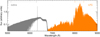 |
Fig. 1 Spectrum of I2 absorption and the LFC as obtained with the FTS. Light of the two sources is combined with a dichroic beam splitter; at wavelengths shorter than 6800 Å, only light from the I2 absorption enters the spectrometer (gray). At longer wavelengths, the spectrum includes only the LFC spectrum (orange). The I2 spectrum follows the intensity of the illuminating lamp and shows the molecular absorption band structure with only very weak lines at long wavelengths beyond 6600Å (T ≈ 44°C). The feature at 6330Å is the HeNe reference laser of the FTS, and the dip at 6500 Å is caused by the transmission curve of the beam splitter. The LFC spectrum is highly dynamic and provides lines across the entire wavelength range and particularly strong lines in the range 8000–8400 Å. Wavelength ranges used for Doppler measurements in the I2 and LFC spectra are indicated with dashed lines at the top. |
2.2 Laser frequency comb
The frequency spectrum of an LFC is a broadband comb of equidistant emission lines, which can be stabilized with high accuracy and precision (Reichert et al. 1999; Diddams et al. 2000; Jones et al. 2000). The position of each line is determined by two degrees of freedom: the repetition rate, frep , and the carrier-envelope-offset frequency, fCEO , governed by the relation
 (1)
(1)
in frequency units, or λn,LFC = c/fn,LFC in units of wavelength. Accuracy and precision are achieved by phase locking frep and fCEO to a stable reference oscillator, such as an atomic clock. LFCs are important tools in metrology and, among many other applications (Diddams 2010; Picqué & Hänsch 2019), are promising calibration light sources for astronomy (Herr & McCracken 2019; Probst et al. 2020; Schmidt et al. 2021). In the following, we will use the expression “absolute calibrator” to indicate that the calibration is traced back to the definition of second as much as the actual setup will allow.
The LFC in our setup is a LaserQuantum (Novanta) tac- cor comb. The source laser is a pulsed Ti:sapphire laser with a repetition rate of approximately 1 GHz. The commercial setup includes an f-2f interferometer for measuring the offset frequency. Two frequency generators (Rohde & Schwarz SMB100A and HMF2500) are used for locking frep and fCEO , respectively. Our time base reference is a GPS-8 from MenloSystems with a precision and accuracy of better than 10−12 in one second, which provides a 10 MHz signal for both frequency generators. For the measurements in this work, the two degrees of freedom of the LFC were stabilized to frep = 1.0019850000 GHz and fCEO = 377.4000000 MHz.
To generate a supercontinuum, we use a photonic crystal fiber stub of 14.5 mm in length (NL-2.8-850-02) tapered by Vytran according to specifications retrieved from simulations based on the approach of Ravi et al. (2018). Our simulation approach is designed to generate a stable supercontinuum, as detailed in Debus (2021).
2.3 Absorption cell with molecular I2
Our iodine absorption cell setup consists of off-the-shelf components from Thorlabs: The iodine cell is a GC19100-I, and the heater assembly is a GCH25-75 controlled with a TC200-EC unit. We use a fiber-coupled tungsten-halogen lamp (HL-2000- HP-FHSA, OceanOptics) with OAP fiber couplers (RC08FC- P01, Thorlabs) to guide light through the cell. The whole optical assembly is wrapped in aluminum foil and placed in a styrofoam insulated box for additional temperature stability. Typically, the temperature is stable to within 100 mK on the timescale of one day.
2.4 Model of molecular iodine absorption
The model we use for molecular iodine absorption is based on a description of the rovibronic structure of the I2 B-X spectrum calculated from molecular potentials for the two electronic states and their hyperfine parameters informed by high-precision measurements of the B-X spectrum of I2 in the visible (Knöckel et al. 2004). Depending on the temperature assumed in the modeling, relative intensities of individual transitions are predicted. The expected accuracy of the transition frequencies is better than 3 MHz (~2m s−1) in the wavelength range of 5260-6670 Å. From the line list, we construct a model spectrum through broadening each individual spectral line according to temperature Doppler broadening and the FTS instrument profile.
For the measurement used in this work, we computed the line list according to an I2 temperature of T = 44 °C. The model spectrum contains a total number of 4 427 241 lines in the range of 5150–6300 Å. We included all lines in our model regardless of their predicted absorption intensity. The I2 spectrum contains on average between 30 and 100 lines per 1 km s−1 Doppler width, which is 100–300 lines in one resolution element seen by a typical astronomical spectrograph (R = 100000). We scale all line intensities from the model calculations by a factor of 3800 to approximately match our observed spectrum.
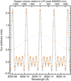 |
Fig. 2 Zoom onto a spectrum of the LFC as observed with the FTS (orange circles with vertical bars for the estimated uncertainty) compared to the analytical description of the FTS instrumental line shape convolved with the LFC peak pattern around the comb tooth n = 362 659 (solid line). For comparison, the instrumental line shape of a spectrograph with a resolution of R = 100 000 is shown (dashed line). |
3 Observational data and frequency calibration
3.1 LFC and I2 spectra
We combined light from an LFC and an I2 absorption cell and simultaneously obtained their spectra in the same FTS scan. A dichroic beam splitter separated the light such that the FTS received light at wavelengths of shorter than 6800 Å only from the I2 cell and at longer wavelengths only from the LFC. We obtained 19 spectra with ten scans each on May 25, 2023; the total scan time per spectrum was 22 minutes. One example spectrum with both components is shown in Fig. 1.
The simultaneous observation of I2 and the LFC spectrum allows a direct comparison between the LFC line positions and the absolute I2 line frequencies. From the information about the LFC line position, we determined the zero-point offset of the FTS frequency solution establishing an accurate frequency scale for the I2 spectrum.
3.2 Absolute frequency calibration from LFC spectrum
We aim to determine the zero-point of our combined I2 and LFC spectra from the region of the spectra containing the strongest LFC lines (Fig. 1). We show a small portion of one LFC spectrum in Fig. 2 that we use as example for the 19 spectra incorporated in the final analysis. The width of the individual lines is determined by the maximum optical path difference, L. We used L = 136 cm as a compromise between spectral resolution and scan time. We compare the spectral region around the LFC peak n = 362 659 to an analytical model of the instrumental line shape convolved with a model LFC peak pattern. The instrumental line shape is a sinc-function with a width determined by the maximum optical path difference. Additional broadening caused by the finite-sized aperture is introduced by a convolution with a box function of width 1/2L (Davis et al. 2001). Assuming optimum aperture, we estimated the effective resolution as the quadratic sum of the effects from finite scan length, L, and corresponding aperture;  at wavenumber k = 12 121 cm−1 (λ = 8250 Å) and using
  . We did not attempt any shape optimization to account for optical imperfections.
The observed spectrum computed from the interferogram is shown with uncertainties estimated from the spectral noise determined in the spectral range of 6600–6700 Å, which is almost completely free of spectral features. The root mean square (rms) noise is σrms = 0.012 in the flux units shown in Fig. 1. The rms noise is independent of the pixel sampling of our spectrum and represents the case of uncorrelated sampling only if the number of pixels, N, is equal to the number of resolution elements, NL ; that is, if the wavenumber stepsize is Δk = ΔkL, with wavenumber k = 1/λ and λ the wavelength. To scale the noise level to our oversampled spectrum, we computed the noise following the scaling relation
 (2)
(2)
where Δk is the stepsize in the spectrum used.
For the LFC spectrum in Fig. 2, absolute peak positions are known from Eq. (1), and peak intensity is adjusted manually to visually match the observed spectrum; we did not attempt to perform a formal fit here. The only additional free parameter of the observed spectrum is the global zero-point offset.
The analytical description of the instrumentally broadened LFC spectrum matches the (offset corrected) observed spectrum to a high degree. The individual LFC peaks show a clear sinc pattern in which the sidelobes partially overlap between the peaks, producing a periodic pattern that is significantly different from noise. We refrain from a detailed analysis of the FTS instrumental line shape but note a slight asymmetry between the depths of the blue and red minima visible around the main peaks; for example, the red minima are less deep and do not fully extend to the expected depth. For comparison, we include in Fig. 2 an instrumental line shape according to a resolution of R = 100 000, the typical resolution of astronomical high-resolution spectrographs (dashed line). Very often, in astronomical spectra, such a resolution element is sampled with an element of approximately 3 pixels per resolution. This underlines the potential of the Fourier transform technique to offer an improved understanding of calibration source characterization and line center fitting.
We determined the zero point (i.e., the offset to the control laser in the FTS) of our observation, 30, from 17 807 individual LFC peaks in the wavelength range of 8000–8400 Å. For every known LFC peak, λn,LFC in Eq. (1), we fit a sinc function to the observed spectrum in a window of 250 m s−1 in Doppler width around the peak center, which approximately covers the main peak of the instrumental line shape. Fit parameters were the amplitude of the LFC peak, the velocity offset between the peak center observed in the spectrum (λn,FTS) and its true position (λn,LFC), vn = c (λn,FTS − λn,LFC)/λn,LFC, and the width of the sinc function. We ignored the additional (symmetric) broadening from the finite aperture applied in the FTS because its main effect is an increase in the peak width. The individual line positions were fit with an uncertainty depending on peak flux; 69 and 34% of the lines showed uncertainties of below 1 m s−1 and below 50 cm s−1, respectively.
The distribution of individual LFC peak position measurements across the spectral range is shown in the left panel of Fig. 3. Peak position measurements are scattered around a mean value with a distribution that is wider at regions of lower peak amplitude, which is consistent with the assumption that lines with higher intensity are better determined. We fit a linear slope to the velocity offsets, vn , to determine the zero point of our I2 and LFC spectrum, v0 , and to search for a potential slope in the wavelength solution, s, using the linear model
 (3)
(3)
with λc = 8200 Å.
In the spectrum shown in Fig. 1, we find a zero-point offset of v0 = 23.945 ± 0.004 m s−1, that is, the statistical uncertainty of the mean wavelength accuracy of our spectrum is  , which is representative of all 19 spectra. The slope we determine from the fit is s = −0.49 ± 0.05 mm s−1 Å−1, which is a (formally) statistically significant slope of around 20 cm s−1 over the range of 400 Å. We experimented with different wavelength ranges, finding that the value of the slope scatters around zero depending on the choice of range. From this we conclude that the slope value is dominated by systematic rather than statistical uncertainties and that our results are consistent with zero slope or smaller than |s| = 1 mm s−1 Å−1 (approximately 3 · 10−8 lin. dispersion). This is in agreement with the results in Huke et al. (2019), where we found the linear dispersion to be below 10−8 at wavelengths of 8000–9800 Å. Following the same argument, we estimate that the uncertainty in the zero-point determination is approximately 1 cm s−1 , which is slightly larger than the formal fit result because of systematic effects.
To assess whether the fit positions were influenced by systematic effects, we investigated the distribution of vn around v0 , divided by their fit uncertainty σn . This distribution is shown in the right panel of Fig. 3. It is consistent with a Gaussian distribution with a width that is only 5% larger than expected from the uncertainties, which is an indication of a realistic noise estimate. To search for wavelength-dependent patterns in the offset, we overplot the weighted means in bins of 5 Å in width in the left panel of Fig. 3 (gray circles). These values scatter around the overall mean with a standard deviation of 16 cm s−1 without evidence for clear systematic uncertainties. From this, we can rule out systematic patterns of several tens of angstroms in length and exceeding a few 10 cm s−1 in the wavelength range of 8000–8400 Å. We note that hidden systematic uncertainties can be caused by the fact that we ignore the additional finite-aperture broadening, imperfections of the instrumental line shape, blends caused by the far wings of the instrumental line shape, or by spectral features like water-absorption, which are not taken into account.
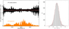 |
Fig. 3 Measurements of LFC line positions. Left: measurements of 17,807 individual LFC peak positions, vn (black circles). Weighted means for bins of 5 Å in width are shown as gray circles. A linear fit to all measurements is shown as a red line; the small slope determined is not visible on this scale. The spectrum of the LFC is overplotted (orange) in linear arbitrary units. The width of the LFC peak position distribution is wider in the areas of lower signal. Right: histogram of residuals between observed and true LFC positions, vn , after subtracting the FTS zero point, v0 and normalized by the uncertainty of the measured line position, σn . The red curve indicates a Gaussian distribution with a 2σ interval indicated by the red vertical bars. The distribution is only 5% broader than expected from uncertainties, σn. |
4 Analysis of model I2 absorption spectrum
4.1 Absolute frequencies
With the zero-point determination, we established an accurate frequency solution for our combined I2 and LFC spectra, which means that the frequency solutions of our iodine spectra were calibrated with an overall uncertainty on the cm s−1 level. We compared our observed spectra to synthetic spectra based on the model of Knöckel et al. (2004) and determined remaining Doppler velocity offsets between model and observations, ΔRV. To see whether the offset showed any dependence on frequency, we performed a fit of the I2 model spectrum to our observations in 302 spectral chunks of 200 km s−1 width across the wavelength range of 5150–6300 Å. The chunk size is a compromise between velocity uncertainty per chunk and the spectral resolution of our analysis. We computed the fits for each spectrum after zero-point correction with the LFC and averaged the results from 19 spectra. For each chunk, fit parameters were the Doppler velocity offset between the model and the observed spectrum, a scaling parameter for the I2 line absorption intensity, and a linear slope for continuum normalization. Uncertainties of the offsets for each chunk per single spectrum, as calculated from the spectrum noise, were below 2m s−1 for 32% and below 4 m s−1 for 90% of the 19 · 302 = 5738 individual computations. After averaging over the 19 exposures, the median uncertainty per chunk is 0.54 m s−1 with 93% of the values below 1m s−1. This allows us to investigate the accuracy of the model’s absolute frequency scale and its dependence on wavelength.
The absolute Doppler velocity offsets, ΔRV, between the I2 model spectrum and our observations are shown in Fig. 4. The model frequencies are centered around zero Doppler offset: the frequencies of the LFC-corrected I2 spectra accurately coincide with the model predictions. Specifically, Doppler offsets are distributed within the estimated frequency uncertainty pattern (Knöckel et al. 2004), which is indicated as gray dashed lines in the top panel of Fig. 4. We therefore conclude that the I2 model accurately predicts the I2 absorption line frequencies, and that the model frequencies are useful for an absolute calibration of astronomical spectrographs.
We allow a scaling of the absorption line intensity because we suspect that the calculated transition intensities applying the Franck-Condon principle show deviations from observations that depend on frequency. The middle panel of Fig. 4 shows that the intensities of the vibronic transitions indeed deviate by more than 10% from the average. We confirmed that the systematic variation of the transition frequencies shown in the top panel of Fig. 4 are independent of line intensity by carrying out the same analysis but keeping line intensity constant over all frequencies. This clearly indicates that improvements in the modeling of the spectra should mainly focus on the energy scale (potential functions and hyperfine interaction) and not the intensity (relaxing the Franck-Condon principle).
The pattern in ΔRV consists of one long-period wave overlaid by a rapidly oscillating pattern that coincindes with the I2 absorption band structure. Uncertainties in ΔRV for each chunk are shown in Fig. 4 and demonstrate that the long-period wave and also parts of the oscillating pattern are significantly different from random noise. The amplitude of the long-period wave is approximately 2m s−1, which significantly exceeds the frequency linearity determined from the LFC lines in Fig. 3. While the LFC lines cover a different frequency range, we see no obvious reason why the linearity should be very different in the frequency range used here. A potential source of systematic errors in determinations of radial velocity is the phase correction. We show the reconstructed phase for one of our spectra in Appendix A, in which we find no evidence for a systematic pattern resembling the ΔRV signature. To verify the robustness of the ΔRV pattern, we computed ΔRV using the power spectrum (instead of the phase-corrected spectrum) and found that the ΔRV pattern also appears. This demonstrates that phase errors are an unlikely source of the ΔRV pattern.
We therefore believe that the pattern of Doppler offsets is dominated by systematic shifts in the model frequencies that vary through the rotational bands of the I2 B-X spectrum. We suggest that our observations be used to improve the Doppler offset in the model spectrum for this systematic effect. To visualize and interpolate the offset pattern, we show a spline fit to the velocity offsets after applying a smoothing (red line in top panel of Fig. 4). The spline represents the effective frequency correction required to adjust the model spectrum. This correction provides a frequency solution that is accurate to within 0.5– 1 m s−1 across the range of 5300–6150 Å. We emphasize that this value does not correspond to the average performance for the full wavelength range but applies to every chunk fitted in the spectrum.
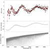 |
Fig. 4 Doppler velocity offset between the I2 model and observations after zero-point correction. Top: individual Doppler offsets in chunks of 200 km s−1 width (black circles). Gray dashed lines show uncertainty limits as estimated in Knöckel et al. (2004). The red line shows a spline fit to the Doppler offsets showing a systematic pattern in the offsets. Middle: relative I2 line intensities as determined from the fitting procedure (see text). Bottom: observed spectrum of I2 for comparison. |
4.2 Comparison to the high-S/N observation
To complement our comparison between the I2 model and observations, we obtained a deep spectrum of I2 absorption with our FTS. We added 227 individual observations with ten scans each taken Jan 20–24, 2023. Here, we used the symmetric configuration of our FTS with a maximum optical path difference of L = 45 cm, applying forward-backward scanning. Each scan took approximately 24 min, with a total scan time of 92 h. Coaddition was performed without individual zero-point correction because typical shifts of a few m s−1 between consecutive observations are not relevant for our visual comparison. We show the spectrum in the wavelength range of 5502–5504 Å in Fig. 5 together with a model for T = 44°C. The S/N of the co-added spectrum in this wavelength range is approximately 2400 at a resolution R = 1.2 · 106. The model provides an excellent fit even at this resolution, reproducing essentially all I2 lines. We particularly emphasize the quality at regions where strong lines overlap, which is a good diagnostic of line depths and spectral resolution. We also note that the model reveals some areas with very few lines where an almost clean continuum is visible. In these regions, the data show a ripple pattern that we believe is not caused by noise but by the sinc function instrumental line shape. Our model includes the instrumental line shape but we did not attempt to empirically determine the line shape, nor did we search for any missing lines or lines underestimated in the model spectrum.
5 Discussion
5.1 Absolute cross calibration with an FTS
The linearity of the FTS frequency scale allowed us to project the frequency accuracy of the LFC onto the wavelength range of the I2 spectrum. The simultaneous (dichroic) observation of LFC and I2 spectra at different wavelengths provides I2 spectra on a frequency scale that is linear and accurate with an offset uncertainty of smaller than Δv0 = 1 cm s−1 (Δv0/c = 3 · 10−11). In general, an FTS can project the accuracy of an absolute frequency standard, for example, an LFC or an I2 spectrum, into wavelength ranges not originally covered by the frequency standard. The projection of frequency accuracy can be carried out on the spectrum from any light source, in particular wavelength reference spectra optimized for astronomical spectrographs, such as an FP.
Such reference spectra can then be used to calibrate astronomical spectrographs in close analogy to the strategy followed when employing an LFC but without the need for the LFC light to cover the entire wavelength range or enter the spectrograph. This significantly relaxes requirements on bandwidth, free spectral range, and peak uniformity (albeit peak stability should not vary strongly on timescales of the FTS scan). For example, the comb teeth of a 1 GHz LFC as used in our setup can be adequately distinguished at 8500 Å by an FTS with a maximum pathf olarger than 30 cm, and the resolution of such an FTS at 6000 Å, R = 106, is sufficient for the characterization of the reference spectrum.
Furthermore, all calibration sources can be characterized at spectral resolutions far exceeding that of the astronomical spectrograph, and can be monitored for variability. This can lift the paradoxical situation whereby spectra from calibration sources are never seen with any other instrument than the one being calibrated.
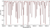 |
Fig. 5 Comparison between a deep (92 h) FTS iodine absorption spectrum (black, scan length L = 45 cm) and a model spectrum (red) for T = 44 °C. |
5.2 Calibration concept for astronomical spectrographs
In practice, high-resolution spectrographs are calibrated using a suite of calibration sources. Spectra of an LFC or hollowcathode lamps are taken once or a few times per day providing information about the absolute positions of wavelengths on the detector. In addition, a stable FP is often used to interpolate between hollow-cathode lamp lines (Wildi et al. 2010; Bauer et al. 2015), or extrapolate to wavelengths not covered by the other sources. Some observatories also use the FP simultaneously during science observations to track the spectrograph drift.
We suggest that an FTS can be used to employ any light source in order to provide accurate information about the wavelength solution (Fig. 6). In practice, one would use an absolute standard – such as an LFC – to calibrate the FTS in a limited spectral range outside the range covered by the astronomical spectrograph (e.g., 8000–8400 Å). During each calibration exposure of the astronomical spectrograph, a fraction of the light from the calibration source needs to be channeled into the FTS where a high-resolution spectrum with an accurate frequency solution is obtained in the full spectral range relevant for the astronomical observations, such as 3800–8000 Å. Thus, for every individual exposure taken with the astronomical spectrograph, the FTS provides an accurate frequency solution for any of the calibration sources.
The availability of accurate spectra for each calibration exposure massively relaxes requirements on calibration source stability. For example, with this strategy, an FP only needs to be stable for the duration of the observation because variability becomes visible at the significantly higher spectral resolution of the FTS. We argue that the full characterization of reference spectra during the time of each observation removes critical free parameters during the calibration process that are otherwise not accessible – such as variability in line strengths from hollow cathode lamps or an LFC – and that the opportunity to use any type of calibration source can lead to superior calibration strategies and reliability. For example, a tunable FP could be used to iteratively cover all detector pixels in the astronomical spectrograph if accurate calibration information is available.
For calibration of the FTS offset, an LFC is a viable choice. Alternatively, a stabilized laser could be sufficient, and we demonstrate in the present paper that I2 also provides offset accuracy at the sub-m s−1 level. The actual choice of calibration source and strategy depends on the individual setup but is very flexible. In our solar observatory in Göttingen, we are obtaining spectra of the Sun in the range of 4000–6800 Å with our FTS. The FTS could be calibrated with the LFC but we avoid using the latter for everyday observations for practical reasons. Instead, we calibrate the instrument with simultaneous FP measurements in the wavelength range of 6800–9000 Å. The FP itself is calibrated every day using a simultaneous observation of the FP with I2 at 4000–6800 Å (Debus et al. 2023).
The design of a full calibration plan exceeds the scope of this paper and depends on the actual setup and requirements of the astronomical spectrograph. It is probably realistic to cover the full wavelength range of astronomical spectrographs with one FP and use the FTS spectra to provide sub-m s−1 accuracy. A tunable FP can further improve the wavelength solution while high-finesse FPs could be used to provide narrow emission lines useful for characterizing the instrumental profile over the entire frequency range. The performance of this critical step with respect to an LFC remains to be tested. With the relaxed requirements on absolute calibration and the flexible choice of dichroic beamsplitters, technical solutions are available for a wide range of applications, including visual and infrared spectrographs.
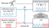 |
Fig. 6 Dichroic calibration concept. The FTS is used to project the frequency scale from the absolute calibrator (shown in red) onto the spectrum of the calibration source (blue), which is used for calibrating the grating spectrograph. |
5.3 Iodine as an absolute calibrator
We demonstrate in Section 4 that spectra computed from the molecular potential model from Knöckel et al. (2004) describe observations taken with an I2 absorption cell to a high degree, and that the modeled and corrected frequencies are accurate to a level of below 1 m s−1 . Thus, iodine cells are useful absolute calibrators, and it is possible to obtain their spectra and wavelength information from (1) FTS measurements or (2) I2 model spectra.
For calibrating astronomical spectrographs, an iodine cell, illuminated by a flatfield lamp, can provide an economic solution in the wavelength range of 5200–6300 Å. This can be useful in addition to other calibration sources, such as hollow cathode lamps and Fabry-Pérot etalons, which are affordable for small-budget observatories. At observatories that include LFCs in their calibration plan, an iodine cell can provide an additional calibration source. Its spectrum more closely resembles stellar absorption spectra and is therefore useful for investigating the impact of potential differences in the trace profiles between emission (LFC/Fabry-Pérot) and absorption spectra (Schmidt et al. 2021). Most importantly, an iodine cell can be operated in the telescope beam, while observing bright stars for example. Thus, accurate iodine cell spectra are useful for verifying Doppler offsets potentially caused from using different light paths for calibration and science light.
Applications involving I2 absorption cell spectra usually rely on reference spectra obtained with an FTS at a significantly higher resolution than used in the astronomical data. Accurate model spectra could be used instead, with the advantage of this being that model spectra are absolutely noise free and can be computed at arbitrary spectral resolution and cell temperature. For example, the model can allow the cell temperature and line intensity (or partial pressure) to be fitted, which can potentially help to reduce requirements on temperature stability and I2 condensation issues. We would always strongly recommend to obtain high-quality reference FTS spectra for any iodine cell used for astronomical spectroscopy. Nevertheless, the flexibility offered by a model spectrum, in addition to the FTS scan, can hardly be overrated as long as the model sufficiently matches the real spectrum.
Our results could also have a very important impact on molecular spectroscopy. To the best of our knowledge, such a complete simulation of a molecular spectrum in connection with an observation has never been achieved over a range of 5200 to 6200 Å with convincing consistency. Our approach can easily be adapted to the modeling of observed molecular spectra.
6 Summary
We obtained simultaneous observations of an LFC and an I2 absorption cell at different wavelengths in an FTS. LFC lines in the wavelength range of 8000–8400 Å were used to test the consistency and linearity of the FTS frequency solution, and to determine offset and dispersion. The dispersion is found to be below 1 m s−1 per 1000 Å, and the offset is determined with an accuracy of 1 cm s−1 . Comparison between the observed spectrum and an analytic model of the instrumental line shape demonstrates exquisite spectral quality at a resolution some 20 times higher than astronomical high-resolution spectra. This allows the development and study of spectral analysis algorithms at the sub-m s−1 level without systematic limitations related to spectral quality.
All individual spectra were zero-point corrected with the information from the LFC lines, and the I2 wavelength range of 5150–6300 Å was used to compare observations against model I2 spectra. The comparison was carried out in spectral chunks of 200 km s−1 width to search for systematic variability in the model line frequencies. The offsets show a characteristic pattern that we attribute to the I2 band structure. The pattern is centered around zero velocity and is consistent with the absolute frequency uncertainty estimated in the model (≲2 m s−1 ). This means that the model spectra are useful for providing an absolute frequency scale in I2 broadband spectra, for example when illuminating an iodine cell with a flatfield lamp or starlight. We argue that the systematic frequency pattern can be corrected from our comparison between model and FTS observations, and that the final frequency scale is accurate within an uncertainty of 1 m s−1 across the wavelength range of 5200–6400 Å. The high consistency between model and observations opens the opportunity to use the high flexibility of model spectra for analysis involving I2 absorption lines.
The high accuracy demonstrated in I2 and LFC spectrometry shows the potential of using an FTS for calibrating astronomical spectrographs. The possibility of obtaining a referenced spectrum from any light source with an FTS allows the spectra of any calibration source to be obtained with an absolute frequency scale known with an uncertainty of better than 10 cm s−1. We argue that simultaneous FTS monitoring of calibration sources alleviates the need for an absolute calibrator to cover the entire frequency range. The FTS can extend the frequency accuracy from a small wavelength portion over its entire range. This also allows great flexibility in the design of calibration sources, which will help improve the performance of calibration strategies for the next generation of high-precision Doppler experiments in astronomy.
Acknowledgements
We regret to notify that Horst Knöckel passed away very recently July 2024. He was the main contributor over many years on the spectroscopic work and development of the iodine model, on which our present work is based. He would be delighted to see these fruits of his work. We acknowledge the help of J. Dabrunz with the extraction of line lists from the IodineSpec program, and we thank the anonymous referee for a very helpful report. We thank T. Schmidt, F. Kerber, L. Pasquini, P. Huke, and members of the ELT Working Group Line Calibration for discussions about results and applications. M.D. was funded through the Bundesministerium für Bildung und Forschung (ELT-ANDES, 05A2023).
Appendix A Phase correction
In Fourier Transform Spectrometry, the spectrum is computed through Fourier transform of the measured interferogram. In theory, the interferogram is symmetric around zero mirror displacement, and Fourier transform of the real and symmetric interferogram leads to a real spectrum with no imaginary part, S (k). In practice, however, the interferogram contains noise, its zero point can not be exactly determined and is a function of wavelength, which all leads to a spectrum with complex components,
 (A.1)
(A.1)
This phase error can be corrected under the assumption that the spectrum is real (the imaginary part is zero). The dependence between C(k) and S (k) can be represented by multiplication with a phase that depends on wavenumber, k,
 (A.2)
(A.2)
With C(k) computed from the measured interferogram, one way to reconstruct S (k) is multiplicative phase correction, an algorithm that follows the strategy developed by Mertz (1965, 1967). With
 (A.3)
(A.3)
we can write
 (A.4)
(A.4)
 (A.5)
(A.5)
which is the phase-corrected, real spectrum. We refer to Learner et al. (1995) and Davis et al. (2001) for more detailed descriptions of phase correction. Wrong phase correction can lead to a significant deformation of spectral features and, in particular, to apparent Doppler shifts proportional to the phase error.
For one of our spectra containing I2 and the LFC signal (as in Fig. 1), we show the phase in Fig. A.1. The phase is derived from the data points with highest intensity. For small portions of the spectrum, we select the 20 % of the points that show the highest intensity (black points in top panel of Fig. A.1), and fit a spline curve through their phase, which is shown as red curve in the bottom panel of Fig. A.1.
For phase correction, we used the 47 cm long symmetric part of the FTS. We estimated that at a systematic displacement of 1 m s−1 in spectral features could be caused by a phase error of approximately 0.01 rad (see Davis et al. 2001). A pattern as the one shown in Fig. 4 could be caused by a similar pattern in phase with such an amplitude. The data we used for phase determination is distributed symmetrically around the smoothed curve with a 1-σ width of approximately 0.01 rad, and the statistical uncertainty of the phase per 10 Å bin is ~ 0.001 rad or 10 cm s−1. From this we can conclude that a phase pattern in frequency of 1 m s−1 amplitude would be detectable in our data. As a consistency check, we tested our RV determination using the power spectrum instead of the phase-corrected spectrum. We found the same ΔRV-pattern in this analysis, which confirms that the pattern is stable against errors in the phase correction. In conclusion, we believe that our analysis is robust against systematic errors on the scale of about 10 cm s−1.
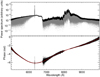 |
Fig. A.1 Top:Power spectrum of the combined iodine and LFC light as in Fig. 1. The top 20 % of the data points are used for phase correction and shown in black. Bottom: Phase reconstructed from the symmetric part of the interferogram following the ’Mertz’ algorithm. The red line shows a spline fit to a running median of the phase data. This smooth curve is used for phase correction. |
References
- Asplund, M., Nordlund, Å., Trampedach, R., Allende Prieto, C., & Stein, R. F. 2000, A&A, 359, 729 [Google Scholar]
- Balthasar, H., Thiele, U., & Woehl, H. 1982, A&A, 114, 357 [NASA ADS] [Google Scholar]
- Baranne, A., Queloz, D., Mayor, M., et al. 1996, A&AS, 119, 373 [NASA ADS] [CrossRef] [EDP Sciences] [Google Scholar]
- Bauer, F. F., Zechmeister, M., & Reiners, A. 2015, A&A, 581, A117 [NASA ADS] [CrossRef] [EDP Sciences] [Google Scholar]
- Bean, J. L., Seifahrt, A., Hartman, H., et al. 2010, ApJ, 713, 410 [NASA ADS] [CrossRef] [Google Scholar]
- Bell, R. J. 1972, Introductory Fourier Transform Spectroscopy (Amsterdam: Elsevier) [Google Scholar]
- Bouchy, F., Pepe, F., & Queloz, D. 2001, A&A, 374, 733 [NASA ADS] [CrossRef] [EDP Sciences] [Google Scholar]
- Butler, R. P., Marcy, G. W., Williams, E., et al. 1996, PASP, 108, 500 [Google Scholar]
- Campbell, B., & Walker, G. A. H. 1979, PASP, 91, 540 [NASA ADS] [CrossRef] [Google Scholar]
- Christensen-Dalsgaard, J. 2004, Sol. Phys., 220, 137 [Google Scholar]
- Davis, S. P., Abrams, M. C., & Brault, J. W. 2001, Fourier Transform Spectrometry (Amsterdam: Elsevier) [Google Scholar]
- Debus, M. 2021, PhD thesis, University of Goettingen, Germany [Google Scholar]
- Debus, M., Schäfer, S., & Reiners, A. 2023, J. Astron. Telesc. Instrum. Syst., 9, 045003 [NASA ADS] [CrossRef] [Google Scholar]
- Diddams, S. A. 2010, J. Opt. Soc. Am. B, 27, B51 [NASA ADS] [CrossRef] [Google Scholar]
- Diddams, S. A., Jones, D. J., Ye, J., et al. 2000, Phys. Rev. Lett., 84, 5102 [NASA ADS] [CrossRef] [Google Scholar]
- Dirac, P. A. M. 1937, Nature, 139, 323 [Google Scholar]
- Einstein, A. 1911, Annal. Phys., 340, 898 [NASA ADS] [CrossRef] [Google Scholar]
- Einstein, A. 1916, Annal. Phys., 354, 769 [NASA ADS] [CrossRef] [Google Scholar]
- Figueira, P., Pepe, F., Lovis, C., & Mayor, M. 2010, A&A, 515, A106 [NASA ADS] [CrossRef] [EDP Sciences] [Google Scholar]
- Fischer, D. A., Anglada-Escude, G., Arriagada, P., et al. 2016, PASP, 128, 066001 [Google Scholar]
- Gerstenkorn, S., & Luc, P. 1978, Atlas du spectre d’absorption de la molecule d’iode 14800-20000 cm-1 (Paris: Editions du Centre National de la Recherche Scientifique (CNRS)) [Google Scholar]
- Gerstenkorn, S., & Luc, P. 1981, Opt. Commun., 36, 322 [NASA ADS] [CrossRef] [Google Scholar]
- Griffin, R., & Griffin, R. 1973, MNRAS, 162, 243 [Google Scholar]
- Griffiths, P. R., & de Haseth, J. A. 2007, Fourier Transform Infrared Spectrometry, 2nd edn. (Hoboken: John Wiley) [CrossRef] [Google Scholar]
- Hajian, A. R., Behr, B. B., Cenko, A. T., et al. 2007, ApJ, 661, 616 [NASA ADS] [CrossRef] [Google Scholar]
- Herr, T., & McCracken, R. A. 2019, IEEE Photon. Technol. Lett., 31, 1890 [CrossRef] [Google Scholar]
- Huke, P., Debus, M., Zechmeister, M., & Reiners, A. 2019, J. Opt. Soc. Am. B, 36, 1899 [NASA ADS] [CrossRef] [Google Scholar]
- Jones, D. J., Diddams, S. A., Ranka, J. K., et al. 2000, Science, 288, 635 [CrossRef] [PubMed] [Google Scholar]
- Kerber, F., Nave, G., & Sansonetti, C. J. 2008, ApJS, 178, 374 [NASA ADS] [CrossRef] [Google Scholar]
- Knöckel, H., Bodermann, B., & Tiemann, E. 2004, Eur. Phys. J. D, 28, 199 [CrossRef] [Google Scholar]
- Koch, A. 1983, PhD thesis, University of Goettingen, Germany [Google Scholar]
- Koch, A., & Woehl, H. 1984, A&A, 134, 134 [NASA ADS] [Google Scholar]
- Kreider, M. K., Fredrick, C., Diddams, S. A., et al. 2022, arXiv e-prints [arXiv:2210.10988] [Google Scholar]
- Learner, R. C. M., & Thorne, A. P. 1988, J. Opt. Soc. Am. B Opt. Phys., 5, 2045 [NASA ADS] [CrossRef] [Google Scholar]
- Learner, R. C. M., Thorne, A. P., Wynne-Jones, I., Brault, J. W., & Abrams, M. C. 1995, J. Opt. Soc. Am. A, 12, 2165 [NASA ADS] [CrossRef] [Google Scholar]
- Lindegren, L., & Dravins, D. 2003, A&A, 401, 1185 [NASA ADS] [CrossRef] [EDP Sciences] [Google Scholar]
- Liske, J., Grazian, A., Vanzella, E., et al. 2008, MNRAS, 386, 1192 [NASA ADS] [CrossRef] [Google Scholar]
- Lo Curto, G., Pasquini, L., Manescau, A., et al. 2012, The Messenger, 149, 2 [NASA ADS] [Google Scholar]
- Lovis, C., & Fischer, D. 2010, in Exoplanets, ed. S. Seager (Tucson, AZ: University of Arizona Press), 27 [Google Scholar]
- Marcy, G. W., & Butler, R. P. 1992, PASP, 104, 270 [Google Scholar]
- Martins, C. J. A. P., Cooke, R., Liske, J., et al. 2024, Exp. Astron., 57, 5 [NASA ADS] [CrossRef] [Google Scholar]
- Mertz, L. 1965, Transformations in Optics (Hoboken: Wiley) [Google Scholar]
- Mertz, L. 1967, Infrared Phys., 7, 17 [NASA ADS] [CrossRef] [Google Scholar]
- Metcalf, A. J., Anderson, T., Bender, C. F., et al. 2019, Optica, 6, 233 [NASA ADS] [CrossRef] [Google Scholar]
- Obrzud, E., Bischof, L., Beltrán, L. M., et al. 2024, SPIE, 13096, 130960A [Google Scholar]
- Picqué, N., & Hänsch, T. W. 2019, Nat. Photon., 13, 146 [CrossRef] [Google Scholar]
- Probst, R. A., Milakovic, D., Toledo-Padrón, B., et al. 2020, Nat. Astron., 4, 603 [NASA ADS] [CrossRef] [Google Scholar]
- Ravi, A., Beck, M., Phillips, D. F., et al. 2018, J. Lightwave Technol., 36, 5309 [NASA ADS] [CrossRef] [Google Scholar]
- Reichert, J., Holzwarth, R., Udem, T., & Hänsch, T. W. 1999, Opt. Commun., 172, 59 [NASA ADS] [CrossRef] [Google Scholar]
- Reiners, A., Mrotzek, N., Lemke, U., Hinrichs, J., & Reinsch, K. 2016, A&A, 587, A65 [NASA ADS] [CrossRef] [EDP Sciences] [Google Scholar]
- Schäfer, S., & Reiners, A. 2012, SPIE Conf. Ser., 8446, 844694 [Google Scholar]
- Schäfer, S., Huke, P., Meyer, D., & Reiners, A. 2020a, SPIE, Conf. Ser., 11447, 114473Q [Google Scholar]
- Schäfer, S., Royen, K., Huster Zapke, A., Ellwarth, M., & Reiners, A. 2020b, SPIE Conf. Ser., 11447, 11447A9 [Google Scholar]
- Schmidt, T. M., & Bouchy, F. 2024, MNRAS, 530, 1252 [NASA ADS] [CrossRef] [Google Scholar]
- Schmidt, T. M., Molaro, P., Murphy, M. T., et al. 2021, A&A, 646, A144 [NASA ADS] [CrossRef] [EDP Sciences] [Google Scholar]
- Schmidt, T. M., Chazelas, B., Lovis, C., et al. 2022, A&A, 664, A191 [NASA ADS] [CrossRef] [EDP Sciences] [Google Scholar]
- Seifahrt, A., Bean, J. L., Kasper, D., et al. 2022, SPIE, 12184, 121841G [NASA ADS] [Google Scholar]
- Steinmetz, T., Wilken, T., Araujo-Hauck, C., et al. 2008, Science, 321, 1335 [Google Scholar]
- Suárez Mascareño, A., Faria, J. P., Figueira, P., et al. 2020, A&A, 639, A77 [Google Scholar]
- Terrien, R. C., Ninan, J. P., Diddams, S. A., et al. 2021, AJ, 161, 252 [NASA ADS] [CrossRef] [Google Scholar]
- Valenti, J. A., Butler, R. P., & Marcy, G. W. 1995, PASP, 107, 966 [NASA ADS] [CrossRef] [Google Scholar]
- Webb, J. K., Flambaum, V. V., Churchill, C. W., Drinkwater, M. J., & Barrow, J. D. 1999, Phys. Rev. Lett., 82, 884 [Google Scholar]
- Wildi, F., Pepe, F., Chazelas, B., Lo Curto, G., & Lovis, C. 2010, SPIE Conf. Ser., 7735, 77354X [NASA ADS] [Google Scholar]
- Wilken, T., Lovis, C., Manescau, A., et al. 2010, MNRAS, 405, L16 [Google Scholar]
- Wu, Y., Huang, Z., Steinmetz, T., et al. 2022, SPIE, 12184, 121841J [NASA ADS] [Google Scholar]
All Figures
|
Fig. 1 Spectrum of I2 absorption and the LFC as obtained with the FTS. Light of the two sources is combined with a dichroic beam splitter; at wavelengths shorter than 6800 Å, only light from the I2 absorption enters the spectrometer (gray). At longer wavelengths, the spectrum includes only the LFC spectrum (orange). The I2 spectrum follows the intensity of the illuminating lamp and shows the molecular absorption band structure with only very weak lines at long wavelengths beyond 6600Å (T ≈ 44°C). The feature at 6330Å is the HeNe reference laser of the FTS, and the dip at 6500 Å is caused by the transmission curve of the beam splitter. The LFC spectrum is highly dynamic and provides lines across the entire wavelength range and particularly strong lines in the range 8000–8400 Å. Wavelength ranges used for Doppler measurements in the I2 and LFC spectra are indicated with dashed lines at the top. |
| In the text | |
|
Fig. 2 Zoom onto a spectrum of the LFC as observed with the FTS (orange circles with vertical bars for the estimated uncertainty) compared to the analytical description of the FTS instrumental line shape convolved with the LFC peak pattern around the comb tooth n = 362 659 (solid line). For comparison, the instrumental line shape of a spectrograph with a resolution of R = 100 000 is shown (dashed line). |
| In the text | |
|
Fig. 3 Measurements of LFC line positions. Left: measurements of 17,807 individual LFC peak positions, vn (black circles). Weighted means for bins of 5 Å in width are shown as gray circles. A linear fit to all measurements is shown as a red line; the small slope determined is not visible on this scale. The spectrum of the LFC is overplotted (orange) in linear arbitrary units. The width of the LFC peak position distribution is wider in the areas of lower signal. Right: histogram of residuals between observed and true LFC positions, vn , after subtracting the FTS zero point, v0 and normalized by the uncertainty of the measured line position, σn . The red curve indicates a Gaussian distribution with a 2σ interval indicated by the red vertical bars. The distribution is only 5% broader than expected from uncertainties, σn. |
| In the text | |
|
Fig. 4 Doppler velocity offset between the I2 model and observations after zero-point correction. Top: individual Doppler offsets in chunks of 200 km s−1 width (black circles). Gray dashed lines show uncertainty limits as estimated in Knöckel et al. (2004). The red line shows a spline fit to the Doppler offsets showing a systematic pattern in the offsets. Middle: relative I2 line intensities as determined from the fitting procedure (see text). Bottom: observed spectrum of I2 for comparison. |
| In the text | |
|
Fig. 5 Comparison between a deep (92 h) FTS iodine absorption spectrum (black, scan length L = 45 cm) and a model spectrum (red) for T = 44 °C. |
| In the text | |
|
Fig. 6 Dichroic calibration concept. The FTS is used to project the frequency scale from the absolute calibrator (shown in red) onto the spectrum of the calibration source (blue), which is used for calibrating the grating spectrograph. |
| In the text | |
|
Fig. A.1 Top:Power spectrum of the combined iodine and LFC light as in Fig. 1. The top 20 % of the data points are used for phase correction and shown in black. Bottom: Phase reconstructed from the symmetric part of the interferogram following the ’Mertz’ algorithm. The red line shows a spline fit to a running median of the phase data. This smooth curve is used for phase correction. |
| In the text | |
Current usage metrics show cumulative count of Article Views (full-text article views including HTML views, PDF and ePub downloads, according to the available data) and Abstracts Views on Vision4Press platform.
Data correspond to usage on the plateform after 2015. The current usage metrics is available 48-96 hours after online publication and is updated daily on week days.
Initial download of the metrics may take a while.