| Issue |
A&A
Volume 690, October 2024
|
|
|---|---|---|
| Article Number | A222 | |
| Number of page(s) | 19 | |
| Section | Cosmology (including clusters of galaxies) | |
| DOI | https://doi.org/10.1051/0004-6361/202451293 | |
| Published online | 10 October 2024 | |
The prototypical major cluster merger Abell 754
I. Calibration of MeerKAT data and radio/X-ray spectral mapping of the cluster
1
INAF – IRA,
via P. Gobetti 101,
40129
Bologna,
Italy
2
Leiden Observatory, Leiden University,
PO Box 9513,
2300 RA
Leiden,
The Netherlands
3
Department of Astronomy, University of Geneva,
ch. d’Ecogia 16,
1290
Versoix,
Switzerland
4
INAF – IASF Milano,
via A. Corti 12,
20133
Milano,
Italy
5
NASA/Goddard Space Flight Center,
Greenbelt,
MD
20771,
USA
6
U.S. Naval Research Laboratory,
4555 Overlook Avenue SW, Code 7213,
Washington,
DC
20375,
USA
7
National Centre for Radio Astrophysics, Tata Institute of Fundamental Research, Pune University,
Pune
411007,
India
★ Corresponding author; andrea.botteon@inaf.it
Received:
28
June
2024
Accepted:
24
August
2024
Context. Abell 754 is a rich galaxy cluster at z = 0.0543 and is considered the prototype of a major cluster merger. As many dynamically unrelaxed systems, it hosts diffuse radio emission on megaparsec-scales. Extended synchrotron sources in the intra-cluster medium (ICM) are commonly interpreted as evidence that a fraction of the gravitational energy released during cluster mergers is dissipated into nonthermal components.
Aims. Here, we aim to use new MeerKAT UHF- and L-band observations to study nonthermal phenomena in Abell 754. These data are complemented with archival XMM-Newton observations to investigate the resolved spectral properties of both the radio and X-ray cluster emission.
Methods. For the first time, we employed the pipeline originally developed to calibrate LOFAR data to MeerKAT observations. This allowed us to perform a direction-dependent calibration and obtain highly sensitive radio images in UHF and L bands that capture the extended emission with unprecedented detail. By using a large XMM-Newton mosaic, we produced thermodynamic maps of the ICM.
Results. Our analysis reveals that the radio halo in the cluster center is bounded by the well-known shock in the eastern direction. Furthermore, in the southwest periphery, we discover an extended radio source that we classify as a radio relic that is possibly tracing a shock driven by the squeezed gas compressed by the merger, outflowing in perpendicular directions. The low-luminosity of this relic appears compatible with direct acceleration of thermal pool electrons. We interpret the observed radio and X-ray features in the context of a major cluster merger with a nonzero impact parameter.
Conclusions. Abell 754 is a remarkable galaxy cluster showcasing exceptional features associated with the ongoing merger event. The high quality of the new MeerKAT data motivates further work on this system.
Key words: radiation mechanisms: thermal / radiation mechanisms: non-thermal / shock waves / galaxies: clusters: general / galaxies: clusters: intracluster medium / galaxies: clusters: individual: A754
© The Authors 2024
 Open Access article, published by EDP Sciences, under the terms of the Creative Commons Attribution License (https://creativecommons.org/licenses/by/4.0), which permits unrestricted use, distribution, and reproduction in any medium, provided the original work is properly cited.
This article is published in open access under the Subscribe to Open model. Subscribe to A&A to support open access publication.
1 Introduction
Mergers between galaxy clusters are among the most energetic events in the Universe (e.g., Sarazin 2002). During these collisions, shocks and turbulence are injected into the intra-cluster medium (ICM) and often generate cluster-wide synchrotron emission with a steep spectrum (e.g., Feretti et al. 2012; van Weeren et al. 2019). Diffuse radio emission in clusters probes a complex hierarchy of novel mechanisms in the ICM that are essentially able to dissipate gravitational energy into relativistic particles and magnetic fields on megaparsec scales (see Brunetti & Jones 2014, for a review). Exploring such a chain of mechanisms has a fundamental impact on our understanding of the microphysics of the ICM and on the evolution of clusters themselves. The study of nonthermal phenomena in merging galaxy clusters is indeed one of the major scientific drivers of many current and future radio interferometers and X-ray microcalorimeters.
Extended synchrotron emission in the ICM is nowadays observed in more than 100 merging clusters of galaxies, and it is broadly classified into radio halos and relics (e.g., van Weeren et al. 2019). Itis currently thought that radio halos trace turbulent regions where relativistic particles are trapped and reaccelerated through scattering with turbulence (e.g., Brunetti et al. 2001; Petrosian 2001; Brunetti & Lazarian 2007, 2016; Miniati 2015; Nishiwaki & Asano 2022). Instead, radio relics originate as a consequence of the particle acceleration and magnetic field amplification ongoing at merger shocks located in cluster outskirts (e.g., Enßlin et al. 1998; Roettiger et al. 1999; Kang et al. 2012; Kang 2020).
In recent years, the advent of the new-generation wide-band interferometers – pathfinders and precursors of the Square Kilometer Array (SKA) – has significantly advanced the discovery of these objects and the characterization of their properties. One of the instruments that is contributing to this advance is MeerKAT (Jonas 2009), which enables deep, broadband, wide-field, (sub-)10″ resolution continuum and polarimetric observations. Observations carried out with MeerKAT allow us to recover the extended diffuse radio emission with a large angular scale of nearby clusters, as well as numerous background sources along the cluster line of sight that can be used as Faraday rotation probes to study the weak ICM magnetic field. Recent studies based on MeerKAT observations have been focused on the analysis of samples of clusters (Knowles et al. 2021, 2022; Kale et al. 2022), radio halos (Venturi et al. 2022; Sikhosana et al. 2023, 2024; Botteon et al. 2023), relics (Parekh et al. 2020, 2022; de Gasperin et al. 2022; Chibueze et al. 2023; Koribalski et al. 2024), mini-halos (Riseley et al. 2022b; Riseley et al. 2023, 2024; Trehaeven et al. 2023), and interaction between ICM and radio galaxies (Ramatsoku et al. 2020; Chibueze et al. 2021; Rudnick et al. 2022; Giacintucci et al. 2022; Velović et al. 2023). These studies showcase the versatile capabilities of MeerKAT in investigating nonthermal phenomena in galaxy clusters.
Recent years have also seen significant leaps forward in the calibration and imaging techniques of radio interferometric data to account for the wide-band and large field of view (FoV) of the new instruments. These developments are crucial to achieving deep images with high dynamic ranges, which are essential for studying the diffuse and faint radio emission from clusters. As a result, MeerKAT data reduction can now benefit from semi-automated calibration pipelines, such as OXKAT (Heywood 2020) and CARACAL (Józsa et al. 2020), while additional optimization steps, such as the correction for direction-dependent effects, can be performed upon user demand to improve the calibration quality even further (e.g., Parekh et al. 2021; Riseley et al. 2022b; Trehaeven et al. 2023). Prior to MeerKAT, significant developments to correct direction-dependent effects have been made for the LOw Frequency ARray (LOFAR; van Haarlem et al. 2013) which, operating at frequencies below 200 MHz, is more affected by ionospheric distortions (e.g., van Weeren et al. 2016, 2021; Williams et al. 2016; Tasse et al. 2018).
Abell 754 (hereafter A754) is a nearby, rich, hot, and massive galaxy cluster in the stage of a violent merger (see Table 1 for a summary of its main properties). It has been actively studied in the optical and X-ray bands and is considered the prototype of a major cluster merger. Previous investigations have unveiled its complex galaxy distribution (Fabricant et al. 1986; Zabludoff & Zaritsky 1995; Godlowski et al. 1998; Okabe & Umetsu 2008), X-ray morphology, and gas temperature structure (Henry & Briel 1995; Henriksen & Markevitch 1996; Markevitch et al. 2003; Henry et al. 2004). These findings suggest a main collision along an east-west axis, probably with a nonzero impact parameter (e.g., Roettiger et al. 1998). Remarkably, A754 is one of the few galaxy clusters where a candidate shock front, appearing as a clear X-ray surface brightness discontinuity a few arcminutes east of the cluster core, was reported with ROSAT (Krivonos et al. 2003). The shock nature of this edge was later confirmed using the Chandra measurement of the temperature jump across the discontinuity, corresponding to a weak shock front with Mach number  (Macario et al. 2011). Signs of nonequilibrium ionization plasma in the ICM due to the shock heating during the merger process have also been reported in the system (Inoue et al. 2016). Early radio observations of A754 provided evidence for ultrarelativistic electrons and magnetic fields within the ICM, making this cluster one of the first known systems hosting extended synchrotron emission (Wielebinski et al. 1977; Mills et al. 1978; Harris et al. 1980). In particular, low-frequency VLA observations at 74 and 330 MHz with the VLA C-array confirmed the existence of a radio halo and suggested the presence of possible radio relics east and west of the radio halo (Kassim et al. 2001). Only the east relic was later confirmed with 1.4 GHz VLA D-array and GMRT observations (Bacchi et al. 2003; Kale & Dwarakanath 2009; Macario et al. 2011). The X-ray detected shock front coincides with the position of the radio relic, which at a low frequency appears connected to the centrally located radio halo (Kale & Dwarakanath 2009; Macario et al. 2011). It is worth noting that these studies were typically conducted with low-resolution (≳60 arcsec) radio imaging, which was necessary to recover the extended diffuse emission using narrow-band data.
A754 is the closest galaxy cluster after Coma that hosts diffuse nonthermal sources in the ICM and a well-characterized merger shock (see, e.g., Bonafede et al. 2021, 2022; Churazov et al. 2021, 2023, for recent work). Its redshift of z = 0.0543 provides a good compromise for performing spatially resolved studies while still allowing us to cover its outskirts with a modest number of pointings with different facilities (for reference: r500 ≃ 21.2 arcmin). For these reasons, A754 is an attractive laboratory in which to investigate the physical processes leading to the dissipation of kinetic energy during cluster mergers in great detail over a wide range of scales. We recently targeted A754 with MeerKAT UHF (544–1088 MHz) andL (856–1712 MHz) band observations, and this paper represents the first in a series dedicated to exploiting these data. In the first part, we focus on the new strategy used to calibrate the MeerKAT data, employing the pipeline originally developed to calibrate low-frequency LOFAR observations. In the second part, we present and discuss our scientific results, complementing the new MeerKAT data with archival XMM-Newton observations.
In this work, we adopted a ΛCDM cosmology with ΩΛ = 0.7, Ωm = 0.3 and H0 = 70 km s−1 Mpc−1, in which 1 arcsec corresponds to 1.056 kpc at the cluster redshift and the luminosity distance is DL = 242.2 Mpc. We adopted the convention Sν ∝ ν−α for radio synchrotron spectrum, where Sν is the flux density at frequency ν and α is the spectral index.
Properties of A754 derived from the literature.
2 MeerKAT data reduction
To process the MeerKAT observations we used the method of van Weeren et al. (2021), employing the facetselfcal.py1 pipeline. This calibration pipeline mainly uses the Default PreProcessing Pipeline (DP3; van Diepen et al. 2018) and WSCLEAN (Offringa et al. 2014); and the losoto2 (de Gasperin et al. 2019), ddf-pipeline3 (Shimwell et al. 2019; Tasse et al. 2021), and python-casacore4 (Casacore Team 2019) packages.
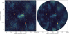 |
Fig. 1 Primary beam corrected images produced by the SDP continuum pipeline for the rising tracks in UHF (left) and L (right) band. |
2.1 Observation setup
Our observing program on A754 (Proposal ID: SCI-20220822- AB-01) made use of MeerKAT UHF- and L-band receivers for a total time of 20 h. The 10 h of observation in each band was split into 5 h observing runs, two “rising“ tracks on 2023 January 6 and 7 (Capture Block IDs: 1673038580 and 1673124676) and two “setting” tracks on 2023 March 25 and 26 (Capture Block IDs: 1679769376 and 1679855479), to maximize the uv coverage on the target. Data were recorded using 4096 channels covering the frequency ranges 544–1088 MHz (UHF band) and 856–1712 MHz (L band) and adopting an integration time of 8 s.
For each observing run, two 10 min scans separated by roughly 3 h were performed on the bandpass calibrator PKS B0407–658. The target A754 was observed with 30 min scans, which were bookended by 2 min observations on the compact source 3C237 to track the time-varying instrumental gains. Additionally, two 5 min scans on the polarization calibrators 3C138 (for the rising tracks) and 3C286 (for the setting tracks) were included. The final on-source time on A754 amounts to 8 h in each band.
2.2 Download of preliminary calibrated data
MeerKAT observations are stored in the archive5 in a data format known as MeerKAT visibility format (MVF). We converted the data into CASA (McMullin et al. 2007; CASA Team 2022) measurement set (MS) format by using the online tool available in the MeerKAT archive, which makes use of the mvftoms.py script of the katdal6 package. In particular, we used the “default calibrated” option of the online tool, which applies a first round of conservative flags produced by the ingest process and all the calibration solutions (including delay, bandpass, and gain) found by the SARAO Science Data Processor7 (SDP) calibration pipeline, which sets the flux density scale according to the model of PKS B0407–658 by Hugo (2021). By default, this option keeps channels in the 163–3885 range. The resulting full polarization MS file we downloaded was ∼1.2 TB in size per observing run. For a quick data quality assessment, we also downloaded the images produced by the SDP continuum pipeline that were available in the archive. In Fig. 1 we show the UHF- and L-band images produced by the pipeline for the two rising tracks. The quality of the images for the setting tracks is comparable.
2.3 Data preparation, averaging, and RFI removal
We used the CASA task split to create new MS files containing only the target field. We then inspected the MS files with the rfigui program of the AOFLAGGER software suite (Offringa et al. 2010, 2012) to flag data affected by radio frequency interference (RFI) and the edge channels that are within the bandpass roll-off. In particular, we found that applying the default flagging strategy to Stokes V is more efficient for flagging RFI present in MeerKAT observations compared to its application to Stokes I, which tends to be too aggressive (see Fig. 2 for a comparison between the two). After having tested the Stokes V flagging strategy on different MeerKAT UHF- and L-band observations, we set it as the default strategy directly in facetselfcal.py (if the user enables the option to run AOFLAGGER on input data).
Before self-calibration, data were averaged by a factor of two in time and by a factor of four in frequency while being compressed with DYSCO (Offringa 2016) to reduce the data volume to a more manageable size of ∽20 GB per MS file. As our scientific analysis is focused on the central region of the field, the time and bandwidth smearing are not an issue.
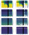 |
Fig. 2 Dynamic spectra of Stokes I and V visibilities of the rising track data of the UHF observation. Plots on the right show the default flagging strategy applied to Stokes I and Stokes V for the shortest (29 m; m000 × m002; top panels) and longest (7.7 km; m048 × m060; bottom panels) baselines (see plot titles). Black bands denote data flagged by the SDP pipeline, while white regions are the data flagged by the AOFLAGGER strategy. |
2.4 Self-calibration
2.4.1 Full field-of-view calibration
As a first attempt to improve the calibration with respect to the images produced by the SDP continuum pipeline (Fig. 1), we performed a self-calibration of the entire MeerKAT FoV. In this and in the following subsections, we use the UHF datasets (which were jointly calibrated) to showcase our results obtained using the facetselfcal.py pipeline described in van Weeren et al. (2021), which was originally developed for the (re)calibration of LOFAR observations from LoTSS. We adopted a similar procedure for the calibration of the MeerKAT L-band observations. We recall that facetselfcal.py uses DP3 to determine calibration solutions and WSCLEAN for imaging.
The self-calibration step consisted of five rounds of “scalarphase+complexgain” calibration. The scalarphase aimed to solve for the polarization-independent (Stokes I) phase correction on a fast timescale of 16 s. These solutions were pre-applied before solving for complexgain, for which we used a solution interval of 3 min, aiming to solve for slow gain variations using a function that depends on time, frequency, and polarization. For both solves, we constrained the solutions to be smooth over frequency by convolving the solutions with a Gaussian kernel of 25 MHz using the smoothnessconstraint parameter in DP3. Outlying amplitude solutions were automatically flagged. Baselines shorter than 500λ were ignored during calibration to filter out the most extended low surface brightness emission from the cluster. During the calibration step, the addition of new columns in the MS files increases their size to ∽90 GB each.
For the imaging, we used the wstacking algorithm (Arras et al. 2021; Ye et al. 2022) and enabled the multiscale multifrequency deconvolution option (Offringa & Smirnov 2017), subdividing the bandwidth into 12 channels. A Briggs robustness weighting of −0.5 (Briggs 1995) was adopted. Data below 10λ were excluded to avoid including auto-correlations that were not flagged8. The bright radio source Hydra A (40.8 Jy at 1.4 GHz; Condon et al. 1998), located at about 3.3° from A754, was included in the image in order to remove its sidelobes affecting the pointing center. Both cleaning masks generated from restored images of previous self-calibration cycles and the auto-masking feature implemented in WSCLEAN were used to guide the deconvolution process. To improve the computational performance of the deconvolution and grid- ding of large images (with ≳108 pixels) from large datasets (with ≳106 visibilities), we enabled the parallel cleaning process (-parallel-deconvolution), which splits into subimages deconvolving them separately, and the baseline-dependent averaging (-baseline-averaging), which averages short baselines more than long baselines.
In Fig. 3a we show the image with the SDP continuum pipeline calibration, with the additional Stokes V flagging and reimaged with WSCLEAN as described above, while in Fig. 3b we show the image obtained with facetselfcal.py in last self-calibration cycle. While more extended emission is recovered in the latter image, calibration artifacts are still present around some sources in the FoV. We also note that no appreciable difference or improvement was observed during the five self-calibration rounds.
 |
Fig. 3 Comparison between UHF images obtained with different calibrations. The color scale is the same in all panels. Images are not corrected for the primary beam attenuation. (a) SDP continuum pipeline calibration. (b) Direction-independent calibration on the full FoV (see Section 2.4.1). (c) Direction-independent calibration on the extracted and phase-shifted dataset (see Section 2.4.2); red arrow shows the shift from the original to the new phase center. (d) Direction-dependent calibration (see Section 2.4.3); red polygons show the five facets used for the direction-dependent calibration. The main sources discussed in the paper are labeled. |
2.4.2 Extraction and calibration toward the target
Because the MeerKAT FoV is large and our research focuses on A754 at the center of the field, in our second attempt we aimed to refine the calibration specifically toward this target. This was achieved with a step called “extraction” (van Weeren et al. 2021), which consists of the subtraction of all sources located outside a user-defined squared region containing the region of interest from the visibility data. The model used for the subtraction of these sources is obtained from the last selfcalibration iteration described in the previous section. The model visibility prediction was performed with WS CLEAN. Ideally, the extracting region should not be excessively large (more than, say, 0.5 deg × 0.5 deg) to limit possible direction-dependent distortions due to ionospheric effects. A small extracting region also has the advantage of allowing for fast reimaging in the subsequent analysis. Nonetheless, due to its low-z, A754 appears as a large target in the sky and it hosts diffuse emission of interest even at a significant distance from the cluster center, such as the tailed source C and the diffuse emission southwest of it (see Fig. 3). For this reason, the extraction region we adopted for A754 is large: 1.6 deg × 1.6 deg. After subtraction, the uv data were phase-shifted with DP3 to the center of the extracting region. The shift of about 10.7 arcmin from the original (RA: 09h09m06.69s, Dec.: −09º40′12.50″) to the new (RA: 09h08m57.80s, Dec: −09º50′39.55″) phase center is represented by the red arrow in Fig. 3c.
The self-calibration of the extracted datasets was done as described in Section 2.4.1. Results are reported in Fig. 3c. In this specific case, the calibration does not improve with respect to the full FoV calibration performed before (see Fig. 3b), except in terms of computing speed, as the subtraction of the sources outside the region of interest implies that the new self-calibration rounds could be performed on images with 16 times fewer pixels. As anticipated, the reason of the lack of improvements is due to the presence of direction-dependent effects that could not be corrected for during self-calibration. In general, the user focusing on small targets (or regions) may already find the calibration obtained after this extraction step satisfactory to carry out the scientific analysis. However, for larger targets (or regions of interest) and/or in the presence of significant direction-dependent effects, the procedure outlined in the following subsection is recommended.
2.4.3 Direction-dependent calibration
To address the challenge of correcting for direction-dependent effects, we incorporated the capability to calibrate data across different directions (facets) of the FoV in facetselfcal.py. This functionality was enabled by the recent introduction of the facet-based imaging mode in WSCLEAN (available from v3.0). An example of the application of direction-dependent calibration with WSCLEAN was presented in de Jong et al. (2022) (but see also Sweijen et al. 2022; Ye et al. 2023), which analyzed LOFAR observations at 144 MHz of the cluster pair A399-A401. The method used in de Jong et al. (2022) consisted of finding the solutions across multiple sources in the FoV, which were extracted and self-calibrated independently, and thus of applying the solutions during the facet-based imaging. In the new implementation of facetselfcal.py, a full joint facet calibration is performed. The direction-dependent calibration was carried out on the same extracted datasets discussed Section 2.4.2.
As a first step, we need to define the directions in which to find calibration solutions. These can be internally determined within facetselfcal.py, which makes use of the LSMTool9 package either to determine the directions containing a given target flux or to tesselate the FoV in a given number of facets. Alternatively, the user can provide a list of directions for the tesselation or even a pre-existing facet layout. After performing some rounds of self-calibration with different facet layouts, we adopted the one leading to the best results. This is shown in Fig. 3d and comprises five directions. We used the same layout for the calibration of the L-band observations.
After a first round of direction-independent imaging, calibration solutions were found for each facet. As before, the calibration was of “scalarphase+complexgain” type and consisted of five iterations. However, in this case, the DP3 solves for the model data column of each facet (for the i-direction, facetselfcal.py calls these columns MODEL_DATA_DDi). The addition of new model data columns may significantly increase the data volume. In our case, each MS file reached a size of ~350 GB during the self-calibration step for five directions. Solutions for each solve type are collected in hierarchical data format v5 (HDF5) files, which we merged into a single file (one per MS) using the lofar_helpers10 package (de Jong et al. 2022). This step is required to apply the facet solutions during direction-dependent imaging.
In Fig. 3d we show the image obtained in the last cycle of direction-dependent calibration. In general, the calibration converges after just two cycles, and only for source B is there a further improvement at the third iteration step. Overall, the direction-dependent calibration leads to an enhancement of the image quality (see Fig. 4). Although there is room for potential improvement (note some residual calibration artifacts around sources A, D, and E), we considered this calibration suitable for the scope of this work and did not attempt further refinement (note that artifacts toward sources B and C, which are close to the diffuse emission of our interest, have been sensibly reduced).
2.4.4 Final considerations
Overall, we conclude that the facetselfcal.py pipeline, originally developed in the context of LOFAR observations, can also be successfully used for the calibration of MeerKAT data. However, the type of solve and solution intervals described here may need to be adapted for datasets with different limitations. Our tests performed on the UHF data of A754, for example, suggest that similar calibration results can be achieved by solving only for gain corrections, using solution intervals from a few minutes up to ~1 h and smoothnessconstraint values in the range of ~10-100 MHz, with the faster “scalarcomplexgain” solve type. As these parameters may influence the stability of solutions and the memory footprint of the pipeline on the computing resource, we recommend some consideration when setting them. Depending on the scientific goals and the quality of the observations, the user can decide whether it is necessary to pass through the extraction step (which is advised in most cases to improve the flexibility in the reimaging and analysis) and/or a directiondependent calibration. For A754, we used the data calibrated as described in Section 2.4.3.
2.5 Imaging
After the last self-calibration iteration, the MS files produced by facetselfcal.py are ready for imaging. Conveniently, facetselfcal.py has an option to “archive” the calibrated datasets. It consists of creating new MS files where the COR- RECTED_DATA column obtained during self-calibration is copied into the DATA column of the new files (also in this case, data are compressed with DYSCO). In this way, the archived MS size goes back to ~20 GB. In the case of direction-dependent imaging, the merged HDF5 files are also required. For reference, these were ~ 18 GB for each dataset of A754.
The imaging was carried out similarly to during the calibration, with particular care taken to deconvolve the diffuse emission from the cluster. Primary beam correction was performed within WS CLEAN, which uses the EveryBeam11 library. The images obtained with a robust value of −0.5 have a resolution and rms noise (σ) of 9.5 arcsec × 7.9 arcsec and σ = 5.7 µJy beam−1 at 819 MHz (UHF) and 6.1 arcsec × 5.1 arcsec and σ = 3.1 µJy beam−1 at 1.28 GHz (L). These images are shown in Figs. 5 and 6 in color. In these images, contours are derived from lower resolution images obtained using a Gaussian taper during imaging and where discrete sources were subtracted following the procedure outlined below. Our highest resolution image, which has a beam of 4.9 arcsec × 6.1 arcsec and rms noise of 5.4 µJy beam−1, was obtained using a robust value of −1.0 on the L-band data.
To better measure the flux density of the diffuse cluster emission, we subtracted the contribution of contaminating discrete sources from the uv data. The first step of this procedure consists of constructing a sky model containing only the discrete sources that we want to subtract from the visibilities. This was achieved by generating high-resolution images using a robust parameter of −1.0 and filtering out the most extended emission by imaging baselines longer than 200λ. To ensure that the model included the emission associated with extended radio galaxies, we forced the multiscale clean to use only the scale corresponding to the synthesized beam and delta components. If we were not using the multiscale clean (namely, if we were using only delta components) part of the faint emission associated with radio galaxies would not be captured by the model. Conversely, if we were not limiting the scales used by the multiscale clean, we would risk including part of the low surface brightness radio emission from the cluster in the model. While this significantly helps to isolate and subtract the extended emission from radio galaxies in the image, part of the brightest regions of the cluster extended emission may still be picked up by the deconvolution process, and thus added to the model. Therefore, before predicting the visibilities, we carefully inspected the model images and manually removed components associated with the cluster extended emission. Additionally, we excluded the clean components associated with the brightest and most extended radio galaxies from the model (namely, those that are discussed in Section 4.3), as the subtraction of their complex emission would not be reliable (see, e.g., Botteon et al. 2022b, for a similar argument). The clean components of the model were then subtracted from the uv data and the residual visibilities were deconvolved to produce images with discrete sources subtracted.
The spectral analysis was performed on images with discrete sources subtracted that were obtained by adopting an inner uv cut of 62λ (≃55.5 arcmin), which corresponds to the shortest common baseline of the UHF and L datasets, to ensure that both observations recover the same largest angular scale in the sky. Subsequently, the images were convolved to a common resolution of 25 arcsec × 25 arcsec, corrected for positional offsets, and regridded to the same pixelation to create the spectral index map that is discussed in Section 4. The corresponding error map is reported in Fig. A.1.
More details on the images presented in this work are given in Table 2. The errors on the flux densities reported in the paper take into account both the statistical and systematic uncertainly, which we assumed to be 5 (L) and 15% (UHF) following previous MeerKAT results (Knowles et al. 2021, 2022; Sikhosana et al. 2024).
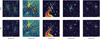 |
Fig. 4 Zoomed-in images of sources A to E (left to right) for the images obtained with the SDP continuum pipeline calibration (top panels) and after direction-dependent calibration with facetselfcal.py (bottom panels). |
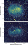 |
Fig. 5 Radio halo recovered with MeerKAT at 819 MHz (UHF, top panel) and at 1.28 GHz (L, bottom panel). The colors show high- resolution images, while the contour represents the 3σ emission from a lower resolution image with discrete sources subtracted (see Table 2 for more details). |
Properties of the images reported in the paper.
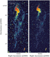 |
Fig. 6 Radio relic recovered with MeerKAT at 819 MHz (UHF, left panel) and at 1.28 GHz (L, right panel). The colors show high- resolution images while the contour represent the 3σ emission from a lower resolution image with discrete sources subtracted (see Table 2 for more details). |
3 XMM-Newton data reduction
3.1 Archival observations
A754 was observed 13 times with XMM-Newton. The four earlier observations took place in 2001 and 2002 (ObsIDs: 0112950301, 0112950401, 0136740101, 0136740201; PI: Turner) and covered the central region of the cluster. In 2008, two deep observations targeted the shock region (ObsIDs: 0556200101, 0556200501; PI: Leccardi) and one was offset from the cluster (ObsID: 0556200301; PI: Leccardi). The six latest observations, conducted in 2019 and 2020, covered the cluster outskirts in various directions (ObsIDs: 0821270601, 0821270801, 0844050101, 0844050201, 0844050301, 0844050401; PI: Ghirardini). We downloaded these data from the XMM-Newton Science Archive and processed them using the Scientific Analysis System (SAS v16.1) and the Extended Source Analysis Software (ESAS; Snowden et al. 2008).
3.2 Data analysis and image preparation
The analysis followed the steps detailed in Ghirardini et al. (2019). In particular, we extracted calibrated event files by running the standard event screening chains and then used the tools mos-filter and pn-filter to generate light curves for each detector (MOS1, MOS2, pn) mounted on the European Photon Imaging Camera (EPIC) to remove time intervals affected by soft-proton flares. For each detector, we thus extracted photon-count images, particle background, and exposure maps in different energy bands. The particle background was modeled using mos-spectra and pn-spectra, rescaling the filterwheel-closed data available in the calibration database to match the observed count rate by measuring the high-energy count rate ratio in the unexposed corners of the three detectors and the closed-filter observations. Exposure images were produced with the eexpmap task, which accounts for vignetting, chip gaps, and dead pixels while computing the local effective exposure time. At the end, we mosaicked photon-count images, particle background, and exposure maps for each EPIC detector and ObsID to obtain a large XMM-Newton mosaic of A754. Narrow-band images were used to produce thermodynamic maps of the ICM; we refer the reader to Section 3.3 for more details. A broad-band image in the 0.4–7.0 keV energy band was used instead to produce the adaptively smoothed and exposure-corrected mosaic reported in Fig. 7. While summing the exposure map of each detector, we rescaled the pn exposure maps in MOS units by multiplying them for a factor representing the ratio of pn to MOS effective areas. This is an energy-dependent factor that was computed for each considered band, taking into account the different response of the 2008 observations, which employed the thick filter instead of the medium filter (as is the case for the others). We note that this rescaling holds when narrow energy bands are used; for the 0.4–7.0 keV range, it represents the average correction factor across the broad band. For this reason, the image shown in Fig. 7 was used only for visualization purposes. The total exposure map given by the sum of MOS1, MOS2, and pn detectors, after soft protons cleaning procedure, is reported in Fig. A.2.
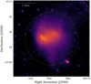 |
Fig. 7 XMM-Newton mosaic in the 0.4–7.0 keV energy band, adaptively smoothed and exposure corrected. The dashed circle denotes r500. |
3.3 Thermodynamic maps
We produced thermodynamic maps of the ICM from the XMM- Newton data following the procedure outlined in Niemiec et al. (2023), and this is summarized as follows. We started by generating photon-count, exposures, and background mosaics in five energy bands (0.4–0.7, 0.7–1.2, 1.2–2.0, 2.0–4.0, and 4.0– 7.0 keV) by combing the 13 ObsIDs available on the cluster. Temperature and the other thermodynamic quantities, were determined from the best-fit thermal plasma model, absorbed for the Galactic column density of hydrogen in the direction of A754 (NH = 4.96 × 1020 cm−2; HI4PI Collaboration 2016), derived using spectral model templates in the five considered bands folded with the XMM-Newton response in XSPEC (see also Section 7 in Jauzac et al. 2016). The metallicity was fixed to 0.3 solar. The sky background was modeled using the spectrum extracted in a cluster-free region from ObsID 0556200301, adopting a model that accounts for both a cosmic X-ray background (CXB) component and a foreground component (e.g., Kuntz & Snowden 2000). The CXB was modeled with an absorbed power-law with photon index Γ = 1.46 (De Luca & Molendi 2004). The foreground component was modeled with both a unabsorbed and an absorbed thermal plasma with solar metallicity: the former represents the local hot bubble with a fixed temperature of 0.11 keV, and the latter represents the Galactic halo, for which we found a best-fit temperature of 0.17 keV. We used apec (Smith et al. 2001) as the thermal plasma model and phabs as the photoelectric absorption model, adopting the abundance table from Asplund et al. (2009) and the cross-sections from Verner et al. (1996).
We used the five energy bands to evaluate the spectral energy distribution in adaptively circular binned regions. The radius of these regions, centered on each pixel of the mosaic not contaminated by discrete sources, was determined by accumulating counts in the 0.4–7.0 keV band until the threshold of 2000 counts was reached. Before this step, all images were rebinned by a factor of two to increase the count statistics per pixel. The radii of the circular regions mostly range from 7.5 arcsec in the cluster’s brightest region to 60 arcsec in the outskirts (Fig. A.3), implying that pixels are correlated on these lengths. The temperature, pseudo-entropy and pseudo-pressure maps are discussed in Section 5. The corresponding error maps are reported in Fig. A.4.
4 Radio emission from A754
The MeerKAT observations of A754 unveil the presence of diffuse emission in form of a radio halo in the central region of the cluster (Fig. 5) and a radio relic in its southwest periphery (Fig. 6), whose properties are summarized in Table 3. Additionally, the images capture a number of bright radio galaxies exhibiting extended emission (Fig. 8). Their position within the cluster can be inferred from Figs. 3d and 9. In the subsequent subsections, we discuss each type of source individually.
4.1 Radio halo
The radio halo in A754 is well-recovered by both our MeerKAT UHF- and L-band high-resolution images of Fig. 5. The emission is mostly elongated in the east-west direction, mirroring the primary merger axis, and exhibits a projected largest linear size of ∽1.6 Mpc. At lower frequency (Fig. 5, top panel), its morphology appears more roundish because of the detection of faint emission in the north-south direction. The most striking feature of the diffuse emission is that its surface brightness rapidly decreases toward the east. Although the detailed analysis of this region will be the subject of our subsequent paper (Botteon et al., in prep.), we anticipate that this feature marks the edge of the radio halo emission, which is bounded by the X- ray detected shock front (Fig. 9). Past observations with limited sensitivity and number of short baselines led to believe that the radio emission at the shock was detached from the central diffuse emission, resulting in its misclassification as a radio relic (Kale & Dwarakanath 2009; Macario et al. 2011). The brightest region of the halo is located to the west, between the radio galaxies LEDA 25746 and LEDA 25701 discussed in Section 4.3.
The integrated flux densities of the radio halo measured from the low-resolution images with discrete sources subtracted12 within an elliptical region encompassing the ∽3σ contour of the UHF image are S0.82 = 457.8 ± 68.7 mJy (UHF) and S1.28 = 223.7 ± 11.2 mJy (L). The integrated spectral index derived from images with a common inner uv cut is α = 1.30 ± 0.39. The k-corrected radio power extrapolated at 1.4 GHz is thus P1.4 = (1.4 ± 0.1) × 1024 W Hz−1, which is in line with the value expected from the known P1.4–M500 relation for radio halos (Cassano et al. 2013; Cuciti et al. 2021).
The spectral index map of Fig. 10 shows that the radio halo does not have a uniform distribution of spectral index values. Flatter spectrum (α ≲ 1.0) emission is found in the west, in the anticipated post-shock region, and in the east, in the region anticipated to have the highest brightness (the typical spectral index error in these regions is ∽0.2; see Fig. A.1). These trace sites of efficient or more recent particle acceleration. Emission with a steeper spectrum (α ≳ 1.5) is instead detected in the north-south direction, perpendicularly with respect to the main cluster merger axis, where particle acceleration is less efficient or occurred long ago (the typical spectral index error in these regions is −0.4; see Fig. A.1).
Properties of the radio halo and relic in A754.
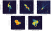 |
Fig. 8 Extended radio galaxies from the highest resolution image at 1.28 GHz (L) that we produced in this work (see Table 2 for more details). |
4.2 Radio relic
New diffuse emission is unveiled in our MeerKAT image in the southwest periphery of A754, at a projected distance of ∽38 arcmin ≃ 2.4 Mpc from the cluster center (Figs. 6 and 9). This source is strongly elongated, with a projected largest-linear size of ∽1.6 Mpc and a 1:7 axis ratio. The emission has a low surface brightness and is irregular, showing some brighter patches and a somewhat straight edge in the southwest direction, while it blends with the emission from the radio galaxy LEDA 25672 (Section 4.3) on the opposite side. A proper characterization of the source morphology, as well as of its flux density and spectral properties, is hampered by its peripheral position in the pointing, which limits the sensitivity of our images due to the primary beam attenuation. With this in mind, the flux densities of the diffuse source that we measured within a polygonal region encompassing the ~3σ contour of the UHF image are S0.82 = 21.8 ± 3.4 mJy (UHF) and S1.28 = 12.5 ± 1.0 mJy (L). The integrated spectral index derived from images with a common inner uv cut is α = 1.24 ± 0.39. The k-corrected radio power extrapolated at 1.4 GHz is thus P1.4 = (8.0 ± 0.7) × 1022 W Hz−1.
We classify this emission as a radio relic because of its peripheral location, elongated morphology, surface brightness apparently declining toward the cluster center, and steep integrated spectrum. Due to the limitations of the images mentioned above, it is not possible to study the resolved spectral properties of the emission (see Fig. 10). The presence of a spectral steepening toward the cluster would further support the interpretation of the source as a relic. Nevertheless, the investigation of this additional property is postponed until better data become available.
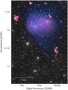 |
Fig. 9 Composite multiwavelength image of A754. Red denotes the radio emission detected with MeerKAT, while blue represents the X-ray emission recovered with XMM-Newton. The background image is from NEOWISE (Mainzer et al. 2014). |
4.3 Extended radio galaxies
In Fig. 8 we show high-resolution images of the five most prominent extended radio galaxies in the proximity of A754. In the following, we briefly comment on them adopting their Lyon-Meudon Extragalactic Database (LEDA; Paturel et al. 1989) number. All the physical lengths quoted below should be intended as projected sizes.
LEDA 25672 (z = 0.0535) is a tailed radio galaxy located ~23 arcmin southwest of the cluster center. The radio emission keeps a collimated and bright structure up to ~150 kpc from its core; then, it bends and bifurcates by roughly 90 degrees, becoming more diffuse. An additional, fainter, isolated filament of emission characterized by α ≳ 2.0 (see Fig. 10) extends for a further ~140 kpc to the southwest. At lower resolution, lower surface brightness emission is recovered around the isolated filament, blending with the newly discovered radio relic (Fig. 6).
LEDA 25701 (z = 0.1590) is a bright background radio galaxy, unrelated to A754, projected at ~10 arcmin to the northwest of the cluster center. It shows a double-lobe structure, extending for ~590 kpc.
LEDA 25746 (z = 0.0487) is projected onto the central region of A754 and is embedded into the radio halo emission. This is a wide-angle, tailed radio galaxy, whose tails appear to bifurcate at ~50 kpc from its core. The radio galaxy emission extends at least for a distance of 150 kpc before blending with the radio halo (Fig. 5). The difference between the galaxy’s line- of-sight velocity and that of A754 is Δvlos ≃ −1680 km s−1, which is larger than the velocity dispersion of cluster galaxies (see Table 1), suggesting the presence of a significant peculiar motion.
LEDA 25790 (z = 0.0585) is a bright, wide-angle, tailed radio galaxy found ~19 arcmin north of A754. The bent jets are well resolved in our image and show the presence of emission knots before inflating the radio lobes, leading to a total source size of ~150 kpc. As before, the line-of-sight relative velocity between the galaxy and A754 of Δvlos ≃ 1260 km s−1 suggests the presence of a significant peculiar motion.
LEDA 25860 (z = 0.0551) is another bright radio galaxy, placed ∼20 arcmin east of A754, showing prominent jets that are separated by a wide angle and inflate radio lobes. The source has a maximum extension of ∼320 kpc.
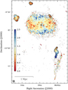 |
Fig. 10 Spectral index map between 819 and 1282 MHz at a resolution of 25″ × 25″. Pixels with values below 3σ were blanked. Contours start from the 3σ level of the UHF image and are spaced by a factor of 2 (see Table 2 for more details). The spectral index error map is reported in Fig. A.1. |
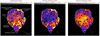 |
Fig. 11 Thermodynamic maps of the ICM with contours from the adaptively smoothed XMM-Newton image of Fig. 7 reported in yellow. Blanked circular regions indicate masked area because of the presence of point sources. |
5 X-ray emission from Abell 754
The large XMM-Newton mosaic of Fig. 7 demonstrates the highly disturbed dynamical state of A754. The cluster has a remnant cool core on the west side which follows the bow shock induced by the cluster merger (Macario et al. 2011). On the opposite side, the X-ray surface brightness possibly shows another rapid surface brightness decrement, which may trace a counter shock. In addition to the east-west features, the X-ray emission shows an elongated tongue of low surface-brigthness emission extending south to a distance of 1.6 Mpc from the cluster center. In order to have a better understanding of the processes undergoing in the thermal gas during the merger, we produced thermodynamic maps of the ICM as described in Section 3.3. These maps, shown in Fig. 11, highlight a number of interesting features, which we label in the left panel and comment on below.
The cluster is hot and exhibits a complex temperature distribution, as previously indicated by temperature maps obtained with ASCA (Henriksen & Markevitch 1996), Chandra (Markevitch et al. 2003; Henriksen et al. 2004), and XMM- Newton (Henry et al. 2004; Laganá et al. 2010, 2019). The brightest ICM region is coincident with the remnant cool core disrupted during the cluster merger, which, as expected, exhibits a lower temperature and entropy than the surrounding gas. The bow-shaped border on the east side of the map delineates the location of the known shock front studied in Macario et al. (2011), where temperature, entropy, and pressure increase due to the shock heating. The rise in thermodynamic values compared to the upstream gas is not very evident in our maps because they are truncated at the position of the shock. While the west region of the cluster has been investigated less, past studies pointed out the presence of high temperature values (see, e.g., Henriksen & Markevitch 1996; Henriksen et al. 2004; Henry et al. 2004; Inoue et al. 2016), which are confirmed by our analysis. In particular, Inoue et al. (2016) proposed that this portion of the cluster may trace a shock-heated region where the plasma is a nonequilibrium ionization state. Our thermodynamic maps are in line with a scenario where a shock front is propagating toward the northwestern cluster outskirts. We have indicated the position of this second putative shock in our temperature map. The presence of a shock front is further supported by both the X-ray and radio emission, which exhibit a rapid decrement (or compression) in this region (Figs. 5 and 7). In addition, the synchrotron radiation here shows a flatter spectrum than the surroundings (Fig. 10), which can also be interpreted in a scenario where particles are (re)accelerated by the passage of a shock front. The southern tongue of low surface brightness emission is characterized by a low temperature, entropy, and pressure. A similar feature with comparable thermodynamic characteristics, which we have labeled as a northern putative tongue, is observed in the opposite direction. In Section 6.1 we use the features discussed above to propose a merger scenario for A754.
6 Discussion
A754 is a prototypical merging cluster at low z hosting nonthermal diffuse radio sources on megaparsec-scales. Thanks to the high sensitivity provided by MeerKAT, these sources have been recovered with unprecedented detail. In particular, the new MeerKAT images show that the emission located at the position of the shock front and previously claimed to be a radio relic (Kale & Dwarakanath 2009; Macario et al. 2011) actually marks the edge of the radio halo. This is not the only case where a shock front is bounding the emission from a halo (see, e.g., Markevitch 2010; van Weeren et al. 2019, and references therein). Recently, other radio edges, not necessarily at the border of the radio emission, have been reported in a number of clusters observed with MeerKAT (Botteon et al. 2023).
The cluster Abell 520 is probably the most extensively studied case of radio halo edge-shock connection (Markevitch et al. 2005; Wang et al. 2018; Hoang et al. 2019). The analysis of such a region and, especially, of the jump in radio emissivity at the front, allows us to determine the origin of the edge; that is, whether relativistic particles are reaccelerated or adiabatically compressed by the shock. A similar discussion for the shock in A754 was also presented by Macario et al. (2011). However, in both cases, determining the physical processes responsible for generating the radio-emitting electrons has remained inconclusive. In our forthcoming work, we will perform a multiband study of the shock front in A754 (Botteon et al., in preparation).
Additionally, the MeerKAT images have unveiled a new extended radio source ∼2.4 Mpc southwest of the cluster center, which we have classified as a radio relic. Relics are the tracers of particles (re)accelerated by shock fronts propagating through the outskirts of clusters during mergers (e.g., Finoguenov et al. 2010; Bourdin et al. 2013; Botteon et al. 2016; Ge et al. 2019; Sarkar et al. 2024). The proximity of the radio galaxy LEDA 25672 (Fig. 6) gives a tantalizing indication of ongoing cosmic-ray seeding, recalling the well-known case of Abell 3411-3412 (van Weeren et al. 2017). Nonetheless, as we discuss more in detail in Section 6.3, the direct acceleration of electrons from the thermal pool is not ruled out in this case. While the distance of the relic in A754 is considerable (∼1.8r500), it is not unique. Other relics exist at comparable or even greater distances from their respective cluster, including those in Abell 2255 (Pizzo et al. 2008; Botteon et al. 2022b), ClG 0217+70 (Brown et al. 2011; Hoang et al. 2021), PLCKESZ G287.0+32.9 (Bagchi et al. 2011; Bonafede et al. 2014), Ant Cluster (Botteon et al. 2021), Coma Cluster (Bonafede et al. 2022), and Bullet Cluster (Sikhosana et al. 2023). Particularly noteworthy is the latter case, which appears as a close analog to A754. Indeed, in both clusters, the peripheral diffuse emission appears in an unusual location relatively to the ICM and to the east-west merger axis that one can infer at first glance from the location of the bow shocks found in the two systems.
In simple head-on collisions, pairs of shocks propagating in opposite directions develop, but the scenario becomes more complex if the merger occurs with a nonzero impact parameter (e.g., Evrard 1990; Roettiger et al. 1993; Ricker & Sarazin 2001). Moreover, recent numerical simulations have indicated that even in nearly head-on collisions, equatorial shocks moving perpendicularly to the merger axis can form (e.g., Ha et al. 2018; Lee et al. 2020; Zhang et al. 2021). Based on the analysis of ROSAT and ASCA data, Henriksen & Markevitch (1996) suggested that A754 is undergoing a slighly off-axis collision. This scenario was later corroborated by tailored numerical simulations (Roettiger et al. 1998). In the following subsection, we use the results obtained in this paper to refine the merger scenario of A754.
 |
Fig. 12 Merger scenario for A754. Top panels: schematic representation of the proposed merger dynamics. (a) Two clusters undergo a slightly off-axis collision nearly in the plane of the sky. (b) As clusters approach, the gas in between is squeezed and propagates in equatorial directions. (c) In the current configuration of A754, tongues of cold and low entropy plasma develop and shock fronts propagate in opposite directions roughly along the merger axis. Bottom panels: temperature slices (for the z projection) from an idealized simulation by ZuHone et al. (2018) of a 1:1 merger with an impact parameter of 500 kpc taken at different times and used to support our sketched merger scenario of A754. |
6.1 Merger scenario
The presence of the sharp discontinuity (shock/radio halo edge) in the east suggests that at least part of the merger motion occurs in this direction. Based on the thermodynamic maps shown in Fig. 11, we suggested the existence ofa second shock likely propagating toward the northwest. Non-planar shocks (i.e., shocks that are not moving in diametrically opposite directions) are distinctive of mergers between clusters with unequal masses colliding with a nonzero impact parameter. In such cases, the shock driven by the less massive cluster curves after the pericenter passage, sweeping through the cluster outskirts (Ricker & Sarazin 2001). The other interesting features highlighted by our thermodynamic maps are the two tongues of low temperature, entropy, and pressure gas developing in the north and south directions, with the latter being more prominent. We interpret these structures as flows originating form the gas between the colliding clusters that is squeezed and expelled in perpendicular directions, accelerating down the pressure gradient (see, e.g., Ricker 1998; Ritchie & Thomas 2002, for early reports of these features in numerical simulations). Also, the asymmetry of the tongues can be interpreted as a non-head-on collision and/or unequal mass ratio.
In light of these results, we propose that A754 is undergoing a major merger as sketched in the top panels of Fig. 12, where two clusters collide with a small impact parameter. The schematic representation delineates how the observed features developed during the merger (gray labels). To support our proposed scenario, we inspected the Galaxy Cluster Merger Catalog (ZuHone et al. 2018). This catalog contains the results from idealized binary cluster mergers exploring a parameter space with different mass ratios and/or impact parameters. In the bottom panels of Fig. 12, we report temperature slices for snapshots at different epochs for the merger with a mass ratio of 1:1 and impact parameter of 500 kpc, where structures similar to those observed in A754 can be identified (gray labels). We remark that the aim of this comparison is not to closely replicate the case of A75413, but to help our understanding of the merger scenario and observed features. In this context, the new relic in the southwest may trace a shock driven by the outflowing gas of the southern tongue. For a sequence illustrating the launch of a shock in that direction by these motions, we invite the reader to consult, for example, Figure 12 in Zhang et al. (2021).
To conclude, the results from the radio and X-ray analysis of the MeerKAT and XMM-Newton data reported in this paper are in line with a major merger between two galaxy clusters undergoing a slightly off-axis collision. Whilst similar features observed in A754 can also be identified in idealized binary merger simulations, we note that in reality departures from these simulations are naturally expected given the cosmological accretion inflows and mergers with clusters containing substructures.
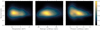 |
Fig. 13 Normalized 2D KDE distributions between spectral index and thermodynamic properties of the ICM, with isocontours drawn at the same levels (0.2, 0.4, 0.6, 0.8). |
6.2 Correlating thermodynamic and spectral index maps
A connection between thermal and nonthermal components in the ICM is expected in the formation models for radio halos (e.g., Brunetti & Jones 2014). Such a connection could be reflected as correlations between the local spectral index of the synchroton radiation and the local thermodynamic properties (temperature, entropy, and pressure) of the thermal gas. Following the argument of Botteon et al. (2020b), in a simplistic scenario where the spectral index reflects the turbulent reacceleration efficiency and the thermal quantities represent the level of heating and mixing in the gas, one may expect regions with a flatter spectral index to correlate with regions with higher values of these properties. However, such investigations have so far only been conducted in a handful of clusters due to the limited availability of suitable X-ray and multifrequency radio data required for this kind of analysis. The search for a correlation between spectral index and temperature was performed in the following systems: Bullet Cluster (Shimwell et al. 2014), A521 (Santra et al. 2024), A2142 (Riseley et al. 2024), A2255 (Botteon et al. 2020b), and A2744 (Orrù et al. 2007; Pearce et al. 2017; Rajpurohit et al. 2021). The findings from these studies are inconclusive, showing a mild to nonexistent correlation between spectral index and temperature. In A2255, there was also an investigation of the relations between spectral index and entropy and pressure, revealing a tendency for flatter spectrum emission to be located in higher entropy regions.
The high quality of the MeerKAT and XMM-Newton observations of A754 allows us to investigate these possible correlations by using an approach that takes advantage of the large angular extent of the cluster and of the method we used to produce the thermodynamic maps of Fig. 11. Our approach consists of correlating the thermodynamic and spectral index maps on a pixel-to-pixel basis and reporting the results as 2D kernel density estimate (KDE) plots, with data weighted by the inverted quadrature sum of the fractional pixel errors. Clearly, the pixels in our maps are correlated, and this method is not suitable for performing a proper statistical analysis (e.g., linear regression). Nonetheless, its advantage is that it condenses the spatial information of two quantities in a single plot, allowing us to search for common (sub)structures in the distribution and provide information on the general trend of the plotted quantities.
In order to correlate the different maps, images were first aligned and regridded to the same pixelation. Pixels covering contaminating X-ray point sources (i.e., the circular regions in Fig. 11) and the extended radio galaxies that were not subtracted from the uv plane (i.e., LEDA 25746 and LEDA 25701) were excluded from the analysis. The resulting 2D KDE plots, normalized for the maximum value of each distribution and obtained from the values of 44,435 pixels, are shown in Fig. 13. While no clear trends can be identified among spectral index and temperature or entropy, evidence of a possible anti-correlation with the pressure is reported. This may indicate that in regions with higher gas pressure, which may be in a higher disturbed state, the acceleration of nonthermal electrons is more efficient, leading to the generation of radio emission with flatter synchrotron spectrum. However, even if a trend may be naively interpreted, we note that the scenario is more complex as (i) these thermodynamic quantities are not good proxies of the turbulence in the ICM; (ii) the timescales of gas heating/cooling and particle acceleration/cooling are different; and (iii) the degree of plasma collisionality, albeit poorly understood, likely affects the acceleration rate. The presence of these relations needs to be validated by further observations and numerical simulations.
6.3 Possibility of a weak radio relic powered by direct acceleration of thermal pool electrons
The radio power of P1.4 = (8.0 ± 0.7) × 1022 W Hz−1 makes the relic in A754 one of the least powerful detected at high frequencies. This adds to the growing number of low-power radio relics that have been discovered lately, especially due to sensitive observations at low frequencies, where steep spectrum sources appear brighter (e.g., Locatelli et al. 2020; Bonafede et al. 2021; Botteon et al. 2021, 2022a; Duchesne et al. 2022; Schellenberger et al. 2022; Riseley et al. 2022a; Jones et al. 2023; Chatterjee et al. 2024; Rajpurohit et al. 2024). Whilst the relic–shock connection is supported by a number of radio/X-ray observations, particle acceleration of thermal pool electrons via diffusive shock acceleration (DSA) is known to be a rather inefficient process for weak shocks (𝓜 ≲ 3) such as those typically found in galaxy clusters (Kang & Jones 2002, 2005). This, combined with the high radio luminosity observed in radio relics, implies untenable acceleration efficiencies of thermal electrons, suggesting that other mechanisms (e.g., reacceleration of suprathermal seed electrons) play a role in most relics (Botteon et al. 2020a). It is therefore interesting to investigate the so-called acceleration efficiency problem for a low-power radio relic such as that in A754, whose large extent suggests that a significant kinetic energy flux is dissipated through the shock surface supporting the nonthermal luminosity of the relativistic electrons radiating in the radio band.
We used the formalism of Botteon et al. (2020a) to derive the electron acceleration efficiency (ηe ) required to reproduce the luminosity of the radio relic as a function of the (unknown) downstream magnetic-field strength (Bd). The computation requires the parameters of the relic (i.e., power and spectral index) and shock (i.e., density, temperature, and surface area). The former are provided by the MeerKAT observations (Table 3). The latter cannot be determined with current X-ray observations as the relic is located outside the FoV of the XMM- Newton mosaic. Therefore, we assumed a shock surface area of 8002π kpc2 , where 800 kpc is the semi-axis of the relic emission, and the density and temperature expected from the universal thermodynamic profiles of Ghirardini et al. (2019), which we consider to be unshocked (i.e., upstream) values. At the distance of the relic in A754 (∽2.4 Mpc ≃ 1.8r500), these are ne ∽ 3 × 10⁻⁵ cm−3 and kT ∽ 3.2 keV. We used the classic DSA formula to compute the shock Mach number from the integrated synchroton spectral index (Blandford & Eichler 1987) and the Rankine-Hugoniot jump conditions to estimate the downstream density and temperature (Landau & Lifshitz 1959).
Our results reported in Fig. 14 indicate that a shock with Mach number 𝓜 = 3.06, corresponding to the central value of our spectral index estimate α = 1.24, can reproduce the luminosity of the radio relic with electron acceleration efficiencies ηe < 10−3 for magnetic field strengths Bd > 0.8 µG. Although the acceleration mechanisms at weak shocks and the magnetic fields in cluster outskirts are still poorly constrained, the values reported here appear reasonable (for Bd ∽ 1 µG, the corresponding thermal-to-magnetic-pressure ratio is βpl ~ 100) and significantly more favorable than those obtained by Botteon et al. (2020a) for a sample of much more powerful radio relics. This suggests that the DSA of thermal electrons represents a viable scenario in A754. We note, however, that if we assume the worstcase scenario allowed by our measurements (i.e., adopting the upper bound of our spectral index measurement (α = 1.63), which leads to 𝓜 = 2.04 under DSA assumptions), the acceleration efficiency required to reproduce the luminosity of the radio relic is significantly higher: ηe < 10−1 for large magnetic field strengths Bd > 4.4 µG, which in turn imply βpl < 2 (see Fig. 14). Efficiencies on the order of 10−1 are generally associated with protons in strong (𝓜 ~ 103) supernova shocks (e.g., Morlino & Caprioli 2012), and thus appear untenable for electrons in weak cluster shocks. Should the radio relic have such a steep spectrum, DSA of thermal electrons would be disfavored compared to a scenario where seed electrons provided by the nearby LEDA 25672 are reaccelerated at the shock, as anticipated in Section 6. Therefore, it will be crucial to better constrain the spectral index of the emission and search for the hypothetical 𝓜 ~ 3 shock with future follow-up observations.
Overall, observations with the new generation of radio interferometers present the tantalizing possibility of uncovering the population of weak relics anticipated by recent numerical work (e.g., Brüggen & Vazza 2020; Zhou et al. 2022; Lee et al. 2024). These relics may be powered by the direct acceleration of thermal pool electrons (e.g., Locatelli et al. 2020) and could have been missed by previous instruments due to their faint emission.
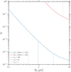 |
Fig. 14 Electron acceleration efficiency that is required to reproduce the radio luminosity of the radio relic in A754 as a function of the downstream magnetic field. Vertical lines denote magnetic field strengths corresponding to different βpl values. |
7 Conclusions
In this paper, we present new MeerKAT data and archival XMM- Newton observations of the prototypical major cluster merger A754. The main outcomes of our work, which is the first in a series dedicated to this target, are outlined below.
From a technical point of view, we tested a new strategy to calibrate MeerKAT observations, adopting the facetselfcal.py pipeline originally developed to calibrate LOFAR data. This method is also considered to be effective for MeerKAT UHF- and L-band observations. Noteworthy features of this scheme include the possibility of improving the calibration toward a specific target of interest through the extraction step, which also enables faster calibration and subsequent reimaging, and to correct for direction-dependent effects across the FoV. This approach allowed us to produce highly sensitive images of A754 at 819 MHz and 1.28 GHz, providing the most detailed view yet of the cluster’s nonthermal emission.
From a scientific point of view, our results can be summarized as follows.
We revised the nature of the diffuse radio emission associated with the well-known shock front detected a few arcminutes east of the cluster core. While this emission was previously classified as a radio relic, our new images reveal that it actually marks the edge of the radio halo, which is bounded by the underlying shock. The integrated spectral index of the halo between 819 MHz and 1.28 GHz is α = 1.30 ± 0.39, implying a radio power at 1.4 GHz of (1.4 ± 0.1) × 1024 W Hz−1. This places it within the known P1.4–M500 relation for radio halos. The resolved spectral index map shows regions of flatter spectrum emission in the east-west direction and steeper spectrum emission in the north-south direction, likely reflecting different efficiencies in particle acceleration along and perpendicular to the main cluster merger axis.
We discovered a new, elongated, peripheral emission at ~2.4 Mpc ≃1.8r500 from the cluster center, which we classified as a radio relic. This emission is detected at both 819 MHz and 1.28 GHz, with an integrated spectral index between these frequencies of α = 1.24 ± 0.39. The radio power at 1.4 GHz of (8.0 ± 0.7) × 1022 W Hz−1 makes it one of the least powerful radio relics observed to date. We found that the DSA of thermal pool electrons represents a viable scenario to explain its origin, unlike what is generally found for more powerful radio relics. Still, we noted the presence of a radio galaxy (LEDA 25672) likely connected to the relic, which may naturally provide supra-thermal electrons, further reducing the electron acceleration efficiency required to explain the relic radio luminosity.
We produced a large XMM-Newton mosaic that allowed us to study the properties of the thermal gas. In particular, we found that the X-ray emission from the ICM shows a prominent elongation toward the south, which we dub “tongue”. Thermodynamic maps suggest that this tongue is constituted of gas with low temperature, entropy, and pressure and that it has a possible counterpart in the northern direction. Signs of shock-heated gas are found in the western region of the cluster, in line with previous X-ray analyses and with the flatter spectrum emission of the radio halo observed in this region.
We interpreted the observed radio and X-ray features in the context of a major cluster-cluster collision with a small impact parameter. Aided by a catalog of idealized simulations of cluster mergers, we propose that in the current phase the gas between the colliding clusters is squeezed and forced to outflow in perpendicular directions, creating the southern tongue and its putative northern counterpart. We speculate that the newly discovered relic may trace a shock driven by this perpendicularly outflowing gas.
We investigated possible correlations between spectral index of the radio emission and thermodynamic properties of the X-ray emitting gas. A possible anti-correlation between spectral index and pressure was noted. This may suggest a scenario where higher pressure regions trace regions with higher acceleration efficiencies, leading to synchrotron emission with a flatter spectrum. Further investigation is needed to confirm (or disprove) these relations and understand their implications for the interplay between thermal and nonthermal components in the ICM.
New-generation radio interferometers combined with novel calibration techniques allow us to obtain radio images of cluster extended emission with unparalleled quality. In combination with complementary X-ray data, these are crucial for unraveling the physics of galaxy cluster mergers. A754, as the prototype of a major cluster-cluster collision, motivates additional work exploiting the new MeerKAT data.
Data availability
The reduced images are available at the CDS via anonymous ftp to cdsarc.cds.unistra.fr (130.79.128.5) or via https://cdsarc.cds.unistra.fr/viz-bin/cat/J/A+A/690/A222
Acknowledgements
We thank the anonymous referee for the comments on the manuscript. We thank André Offringa for responsive support and bug fixes with WSCLEAN and Frits Sweijen for creating the composite image displayed in Fig. 9. A.B. acknowledges financial support from the European Union - Next Generation EU. R.J.vW. acknowledges support from the ERC Starting Grant ClusterWeb 804208. R.K. acknowledges the support of the Department of Atomic Energy, Government of India, under project no. 12-R&D-TFR-5.02-0700 and the SERB Women Excellence Award WEA/2021/000008. Basic research in radio astronomy at the Naval Research Laboratory is supported by 6.1 Base funding. The MeerKAT telescope is operated by the South African Radio Astronomy Observatory, which is a facility of the National Research Foundation, an agency of the Department of Science and Innovation. The scientific results reported in this article are based in part on observations obtained with XMM-Newton, an ESA science mission with instruments and contributions directly funded by ESA Member States and NASA. This work made use of data from the Galaxy Cluster Merger Catalog (http://gcmc.hub.yt). This research made use of the following PYTHON packages: APLpy (Robitaille & Bressert 2012), astropy (Astropy Collaboration 2022), CMasher (van der Velden 2020), iminuit (Dembinski et al. 2024), matplotlib (Hunter 2007), numpy (van der Walt et al. 2011), and scipy (Virtanen et al. 2020).
Appendix A Ancillary images
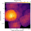 |
Fig. A.2 Exposure map of the XMM-Newton mosaic of A754. It shows the EPIC net exposure in MOS units. |
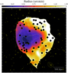 |
Fig. A.3 Map showing the radii of the adaptively binned circular regions. |
References
- Arras, P., Reinecke, M., Westermann, R., & Enßlin, T. A. 2021, A&A, 646, A58 [NASA ADS] [CrossRef] [EDP Sciences] [Google Scholar]
- Asplund, M., Grevesse, N., Sauval, A., & Scott, P. 2009, ARA&A, 47, 481 [Google Scholar]
- Astropy Collaboration (Price-Whelan, A. M., et al.) 2022, ApJ, 935, 167 [NASA ADS] [CrossRef] [Google Scholar]
- Bacchi, M., Feretti, L., Giovannini, G., & Govoni, F. 2003, A&A, 400, 465 [NASA ADS] [CrossRef] [EDP Sciences] [Google Scholar]
- Bagchi, J., Sirothia, S., Werner, N., et al. 2011, ApJ, 736, L8 [NASA ADS] [CrossRef] [Google Scholar]
- Blandford, R. D., & Eichler, D. 1987, Phys. Rep., 154, 1 [NASA ADS] [CrossRef] [Google Scholar]
- Bonafede, A., Intema, H. T., Brüggen, M., et al. 2014, ApJ, 785, 1 [Google Scholar]
- Bonafede, A., Brunetti, G., Vazza, F., et al. 2021, ApJ, 907, 32 [Google Scholar]
- Bonafede, A., Brunetti, G., Rudnick, L., et al. 2022, ApJ, 933, 218 [NASA ADS] [CrossRef] [Google Scholar]
- Botteon, A., Gastaldello, F., Brunetti, G., & Dallacasa, D. 2016, MNRAS, 460, L84 [Google Scholar]
- Botteon, A., Brunetti, G., Ryu, D., & Roh, S. 2020a, A&A, 634, A64 [NASA ADS] [CrossRef] [EDP Sciences] [Google Scholar]
- Botteon, A., Brunetti, G., van Weeren, R. J., et al. 2020b, ApJ, 897, 93 [Google Scholar]
- Botteon, A., Cassano, R., van Weeren, R. J., et al. 2021, ApJ, 914, L29 [NASA ADS] [CrossRef] [Google Scholar]
- Botteon, A., Shimwell, T. W., Cassano, R., et al. 2022a, A&A, 660, A78 [NASA ADS] [CrossRef] [EDP Sciences] [Google Scholar]
- Botteon, A., van Weeren, R. J., Brunetti, G., et al. 2022b, Sci. Adv., 8, eabq7623 [NASA ADS] [CrossRef] [Google Scholar]
- Botteon, A., Markevitch, M., van Weeren, R. J., Brunetti, G., & Shimwell, T. W. 2023, A&A, 674, A53 [NASA ADS] [CrossRef] [EDP Sciences] [Google Scholar]
- Bourdin, H., Mazzotta, P., Markevitch, M., Giacintucci, S., & Brunetti, G. 2013, ApJ, 764, 82 [Google Scholar]
- Briggs, D. 1995, BAAS, 27, 1444 [NASA ADS] [Google Scholar]
- Brown, S., Duesterhoeft, J., & Rudnick, L. 2011, ApJ, 727, L25 [Google Scholar]
- Brüggen, M., & Vazza, F. 2020, MNRAS, 493, 2306 [Google Scholar]
- Brunetti, G., & Jones, T. W. 2014, Int. J. Mod. Phys. D, 23, 30007 [Google Scholar]
- Brunetti, G., & Lazarian, A. 2007, MNRAS, 378, 245 [Google Scholar]
- Brunetti, G., & Lazarian, A. 2016, MNRAS, 458, 2584 [Google Scholar]
- Brunetti, G., Setti, G., Feretti, L., & Giovannini, G. 2001, MNRAS, 320, 365 [Google Scholar]
- CASA Team (Bean, B., et al.) 2022, PASP, 134, 114501 [NASA ADS] [CrossRef] [Google Scholar]
- Casacore Team 2019, Astrophysics Source Code Library [record ascl:1912.002] [Google Scholar]
- Cassano, R., Ettori, S., Brunetti, G., et al. 2013, ApJ, 777, 141 [Google Scholar]
- Cavagnolo, K. W., Donahue, M. E., Voit, G. M., & Sun, M. 2009, ApJS, 182, 12 [NASA ADS] [CrossRef] [Google Scholar]
- Chatterjee, S., Rahaman, M., Datta, A., Kale, R., & Paul, S. 2024, MNRAS, 527, 10986 [Google Scholar]
- Chen, Y., Reiprich, T. H., Böhringer, H., Ikebe, Y., & Zhang, Y.-Y. 2007, A&A, 466, 805 [NASA ADS] [CrossRef] [EDP Sciences] [Google Scholar]
- Chibueze, J. O., Sakemi, H., Ohmura, T., et al. 2021, Nature, 593, 47 [NASA ADS] [CrossRef] [Google Scholar]
- Chibueze, J. O., Akamatsu, H., Parekh, V., et al. 2023, PASJ, 75, S97 [NASA ADS] [CrossRef] [Google Scholar]
- Christlein, D., & Zabludoff, A. I. 2003, ApJ, 591, 764 [Google Scholar]
- Churazov, E., Khabibullin, I., Bykov, A. M., Lyskova, N., & Sunyaev, R. 2023, A&A, 670, A156 [NASA ADS] [CrossRef] [EDP Sciences] [Google Scholar]
- Churazov, E., Khabibullin, I., Lyskova, N., Sunyaev, R., & Bykov, A. M. 2021, A&A, 651, A41 [NASA ADS] [CrossRef] [EDP Sciences] [Google Scholar]
- Condon, J. J., Cotton, W. D., Greisen, E., et al. 1998, AJ, 115, 1693 [NASA ADS] [CrossRef] [Google Scholar]
- Cuciti, V., Cassano, R., Brunetti, G., et al. 2021, A&A, 647, A51 [EDP Sciences] [Google Scholar]
- de Gasperin, F., Dijkema, T. J., Drabent, A., et al. 2019, A&A, 622, A5 [NASA ADS] [CrossRef] [EDP Sciences] [Google Scholar]
- de Gasperin, F., Rudnick, L., Finoguenov, A., et al. 2022, A&A, 659, A146 [NASA ADS] [CrossRef] [EDP Sciences] [Google Scholar]
- de Jong, J., van Weeren, R. J., Botteon, A., et al. 2022, A&A, 668, A107 [NASA ADS] [CrossRef] [EDP Sciences] [Google Scholar]
- De Luca, A., & Molendi, S. 2004, A&A, 419, 837 [NASA ADS] [CrossRef] [EDP Sciences] [Google Scholar]
- Dembinski, H., Ongmongkolkul, P., Deil, C., et al. 2024, scikit-hep/iminuit [Google Scholar]
- Duchesne, S. W., Johnston-Hollitt, M., Riseley, C. J., Bartalucci, I., & Keel, S. 2022, MNRAS, 511, 3525 [NASA ADS] [CrossRef] [Google Scholar]
- Eckert, D., Gaspari, M., Vazza, F., et al. 2017, ApJ, 843, L29 [Google Scholar]
- Enßlin, T. A., Biermann, P., Klein, U., & Kohle, S. 1998, A&A, 332, 395 [Google Scholar]
- Evrard, A. E. 1990, ApJ, 363, 349 [NASA ADS] [CrossRef] [Google Scholar]
- Fabricant, D. G., Beers, T., Geller, M. J., et al. 1986, ApJ, 308, 530 [NASA ADS] [CrossRef] [Google Scholar]
- Feretti, L., Giovannini, G., Govoni, F., & Murgia, M. 2012, A&A Rev., 20, 54 [Google Scholar]
- Finoguenov, A., Sarazin, C. L., Nakazawa, K., Wik, D. R., & Clarke, T. E. 2010, ApJ, 715, 1143 [Google Scholar]
- Ge, C., Sun, M., Liu, R.-Y., et al. 2019, MNRAS, 486, L36 [NASA ADS] [CrossRef] [Google Scholar]
- Ghirardini, V., Eckert, D., Ettori, S., et al. 2019, A&A, 621, A41 [NASA ADS] [CrossRef] [EDP Sciences] [Google Scholar]
- Giacintucci, S., Venturi, T., Markevitch, M., et al. 2022, ApJ, 934, 49 [NASA ADS] [CrossRef] [Google Scholar]
- Godlowski, W., Baier, F., & MacGillivray, H. 1998, A&A, 339, 709 [NASA ADS] [Google Scholar]
- Ha, J.-H., Ryu, D., & Kang, H. 2018, ApJ, 857, 26 [NASA ADS] [CrossRef] [Google Scholar]
- Harris, D. E., Costain, C., Strom, R., et al. 1980, A&A, 90, 283 [NASA ADS] [Google Scholar]
- Henriksen, M. J., & Markevitch, M. 1996, ApJ, 466, L79 [NASA ADS] [CrossRef] [Google Scholar]
- Henriksen, M. J., Hudson, D. S., & Tittley, E. 2004, ApJ, 610, 762 [NASA ADS] [CrossRef] [Google Scholar]
- Henry, J. P., & Briel, U. 1995, ApJ, 443, L9 [NASA ADS] [CrossRef] [Google Scholar]
- Henry, J. P., Finoguenov, A., & Briel, U. 2004, ApJ, 615, 181 [NASA ADS] [CrossRef] [Google Scholar]
- Heywood, I. 2020, Astrophysics Source Code Library [record ascl:2009.003] [Google Scholar]
- HI4PI Collaboration (Ben Bekhti, N., et al.) 2016, A&A, 594, A116 [NASA ADS] [CrossRef] [EDP Sciences] [Google Scholar]
- Hoang, D. N., Shimwell, T. W., van Weeren, R. J., et al. 2019, A&A, 622, A20 [NASA ADS] [CrossRef] [EDP Sciences] [Google Scholar]
- Hoang, D. N., Zhang, X., Stuardi, C., et al. 2021, A&A, 656, A154 [NASA ADS] [CrossRef] [EDP Sciences] [Google Scholar]
- Hudson, D. S., Mittal, R., Reiprich, T. H., et al. 2010, A&A, 513, A37 [NASA ADS] [CrossRef] [EDP Sciences] [Google Scholar]
- Hugo, B. V. 2021, Reference Flux Scale for MeerKAT: Long Term Observation and Field Modelling of PKS B0407-65 (Cape Town: South African Radio Astronomy Observatory) [Google Scholar]
- Hunter, J. D. 2007, Comput. Sci. Eng., 9, 90 [NASA ADS] [CrossRef] [Google Scholar]
- Inoue, S., Hayashida, K., Ueda, S., et al. 2016, PASJ, 68, S23 [NASA ADS] [CrossRef] [Google Scholar]
- Jauzac, M., Eckert, D., Schwinn, J., et al. 2016, MNRAS, 463, 3876 [NASA ADS] [CrossRef] [Google Scholar]
- Jonas, J. 2009, IEEE Proceedings, 97, 1522 [NASA ADS] [CrossRef] [Google Scholar]
- Jones, A., de Gasperin, F., Cuciti, V., et al. 2023, A&A, 680, A31 [NASA ADS] [CrossRef] [EDP Sciences] [Google Scholar]
- Józsa, G. I., White, S. V., Thorat, K., et al. 2020, Astrophysics Source Code Library [record ascl:2006.014] [Google Scholar]
- Kale, R., & Dwarakanath, K. 2009, ApJ, 699, 1883 [NASA ADS] [CrossRef] [Google Scholar]
- Kale, R., Parekh, V., Rahaman, M., et al. 2022, MNRAS, 514, 5969 [NASA ADS] [CrossRef] [Google Scholar]
- Kang, H. 2020, JKAS, 53, 59 [NASA ADS] [Google Scholar]
- Kang, H., & Jones, T. W. 2002, JKAS, 35, 159 [NASA ADS] [Google Scholar]
- Kang, H., & Jones, T. W. 2005, ApJ, 620, 44 [NASA ADS] [CrossRef] [Google Scholar]
- Kang, H., Ryu, D., & Jones, T.W. 2012, ApJ, 756, 97 [NASA ADS] [CrossRef] [Google Scholar]
- Kassim, N., Clarke, T. E., Enßlin, T. A., Cohen, A., & Neumann, D. 2001, ApJ, 559, 785 [NASA ADS] [CrossRef] [Google Scholar]
- Knowles, K., Pillay, D. S., Amodeo, S., et al. 2021, MNRAS, 504, 1749 [NASA ADS] [CrossRef] [Google Scholar]
- Knowles, K., Cotton, W. D., Rudnick, L., et al. 2022, A&A, 657, A56 [NASA ADS] [CrossRef] [EDP Sciences] [Google Scholar]
- Koribalski, B. S., Veronica, A., Dolag, K., et al. 2024, MNRAS, 531, 3357 [CrossRef] [Google Scholar]
- Krivonos, R., Vikhlinin, A., Markevitch, M., & Pavlinsky, M. 2003, Astron. Lett., 29, 425 [NASA ADS] [CrossRef] [Google Scholar]
- Kuntz, K., & Snowden, S. 2000, ApJ, 543, 195 [NASA ADS] [CrossRef] [Google Scholar]
- Laganá, T. F., Durret, F., & Lopes, P. A. 2019, MNRAS, 484, 2807 [CrossRef] [Google Scholar]
- Laganá, T. F., Andrade-Santos, F., & Lima Neto, G. 2010, A&A, 511, A15 [NASA ADS] [CrossRef] [EDP Sciences] [Google Scholar]
- Landau, L., & Lifshitz, E. 1959, Fluid Mechanics (Oxford: Pergamon Press) [Google Scholar]
- Lee, W., Jee, M. J., Kang, H., et al. 2020, ApJ, 894, 60 [NASA ADS] [CrossRef] [Google Scholar]
- Lee, W., Pillepich, A., ZuHone, J. A., et al. 2024, A&A, 686, A55 [NASA ADS] [CrossRef] [EDP Sciences] [Google Scholar]
- Locatelli, N., Rajpurohit, K., Vazza, F., et al. 2020, MNRAS, 496, L48 [NASA ADS] [CrossRef] [Google Scholar]
- Macario, G., Markevitch, M., Giacintucci, S., et al. 2011, ApJ, 728, 82 [NASA ADS] [CrossRef] [Google Scholar]
- Mainzer, A., Bauer, J., Cutri, R. M., et al. 2014, ApJ, 792, 30 [Google Scholar]
- Markevitch, M. 2010, arXiv e-prints [arXiv:1010.3660] [Google Scholar]
- Markevitch, M., Mazzotta, P., Vikhlinin, A., et al. 2003, ApJ, 586, L19 [NASA ADS] [CrossRef] [Google Scholar]
- Markevitch, M., Govoni, F., Brunetti, G., & Jerius, D. 2005, ApJ, 627, 733 [Google Scholar]
- McMullin, J., Waters, B., Schiebel, D., Young, W., & Golap, K. 2007, ASP Conf. Ser., 376, 127 [NASA ADS] [Google Scholar]
- Mills, B., Hunstead, R. W., & Skellern, D. 1978, MNRAS, 185, 51P [NASA ADS] [CrossRef] [Google Scholar]
- Miniati, F. 2015, ApJ, 800, 60 [Google Scholar]
- Morlino, G., & Caprioli, D. 2012, A&A, 538, A81 [NASA ADS] [CrossRef] [EDP Sciences] [Google Scholar]
- Niemiec, A., Jauzac, M., Eckert, D., et al. 2023, MNRAS, 524, 2883 [NASA ADS] [CrossRef] [Google Scholar]
- Nishiwaki, K., & Asano, K. 2022, ApJ, 934, 182 [NASA ADS] [CrossRef] [Google Scholar]
- Offringa, A. R. 2016, A&A, 595, A99 [NASA ADS] [CrossRef] [EDP Sciences] [Google Scholar]
- Offringa, A. R., & Smirnov, O. M. 2017, MNRAS, 471, 301 [Google Scholar]
- Offringa, A. R., de Bruyn, A., Biehl, M., et al. 2010, MNRAS, 405, 155 [NASA ADS] [Google Scholar]
- Offringa, A. R., van de Gronde, J., & Roerdink, J. 2012, A&A, 539, A95 [NASA ADS] [CrossRef] [EDP Sciences] [Google Scholar]
- Offringa, A. R., McKinley, B., Hurley-Walker, N., et al. 2014, MNRAS, 444, 606 [Google Scholar]
- Okabe, N., & Umetsu, K. 2008, PASJ, 60, 345 [NASA ADS] [Google Scholar]
- Orrù, E., Murgia, M., Feretti, L., et al. 2007, A&A, 467, 943 [NASA ADS] [CrossRef] [EDP Sciences] [Google Scholar]
- Parekh, V., Thorat, K., Kale, R., et al. 2020, MNRAS, 499, 404 [NASA ADS] [CrossRef] [Google Scholar]
- Parekh, V., Kincaid, R., Hugo, B. V., Ramaila, A. J., & Oozeer, N. 2021, Galaxies, 9, 90 [NASA ADS] [CrossRef] [Google Scholar]
- Parekh, V., Kincaid, R., Thorat, K., et al. 2022, MNRAS, 509, 3086 [Google Scholar]
- Paturel, G., Fouque, P., Bottinelli, L., & Gouguenheim, L. 1989, A&AS, 80, 299 [Google Scholar]
- Pearce, C., van Weeren, R. J., Andrade-Santos, F., et al. 2017, ApJ, 845, 81 [NASA ADS] [CrossRef] [Google Scholar]
- Petrosian, V. 2001, ApJ, 557, 560 [Google Scholar]
- Pizzo, R. F., de Bruyn, A., Feretti, L., & Govoni, F. 2008, A&A, 481, L91 [NASA ADS] [CrossRef] [EDP Sciences] [Google Scholar]
- Planck Collaboration XXVII. 2016, A&A, 594, A27 [NASA ADS] [CrossRef] [EDP Sciences] [Google Scholar]
- Rajpurohit, K., Vazza, F., van Weeren, R. J., et al. 2021, A&A, 654, A41 [NASA ADS] [CrossRef] [EDP Sciences] [Google Scholar]
- Rajpurohit, K., Lovisari, L., Botteon, A., et al. 2024, ApJ, 966, 38 [CrossRef] [Google Scholar]
- Ramatsoku, M., Murgia, M., Vacca, V., et al. 2020, A&A, 636, L1 [NASA ADS] [CrossRef] [EDP Sciences] [Google Scholar]
- Ricker, P. 1998, ApJ, 496, 670 [NASA ADS] [CrossRef] [Google Scholar]
- Ricker, P., & Sarazin, C. L. 2001, ApJ, 561, 621 [NASA ADS] [CrossRef] [Google Scholar]
- Riseley, C. J., Bonnassieux, E., Vernstrom, T., et al. 2022a, MNRAS, 515, 1871 [NASA ADS] [CrossRef] [Google Scholar]
- Riseley, C. J., Rajpurohit, K., Loi, F., et al. 2022b, MNRAS, 512, 4210 [NASA ADS] [CrossRef] [Google Scholar]
- Riseley, C. J., Biava, N., Lusetti, G., et al. 2023, MNRAS, 524, 6052 [NASA ADS] [CrossRef] [Google Scholar]
- Riseley, C. J., Bonafede, A., Bruno, L., et al. 2024, A&A, 686, A44 [NASA ADS] [CrossRef] [EDP Sciences] [Google Scholar]
- Ritchie, B., & Thomas, P. A. 2002, MNRAS, 329, 675 [NASA ADS] [CrossRef] [Google Scholar]
- Robitaille, T. P., & Bressert, E. 2012, Astrophysics Source Code Library [record ascl:1208.017] [Google Scholar]
- Roettiger, K., Burns, J., & Loken, C. 1993, ApJ, 407, L53 [NASA ADS] [CrossRef] [Google Scholar]
- Roettiger, K., Stone, J. M., & Mushotzky, R. F. 1998, ApJ, 493, 62 [NASA ADS] [CrossRef] [Google Scholar]
- Roettiger, K., Burns, J. O., & Stone, J. M. 1999, ApJ, 518, 603 [Google Scholar]
- Rudnick, L., Brüggen, M., Brunetti, G., et al. 2022, ApJ, 935, 168 [NASA ADS] [CrossRef] [Google Scholar]
- Santra, R., Kale, R., Giacintucci, S., et al. 2024, ApJ, 962, 40 [NASA ADS] [CrossRef] [Google Scholar]
- Sarazin, C. L. 2002, Astrophys. Space Sci. Lib., 272, 1 [NASA ADS] [Google Scholar]
- Sarkar, A., Andrade-Santos, F., van Weeren, R. J., et al. 2024, ApJ, 962, 161 [NASA ADS] [CrossRef] [Google Scholar]
- Schellenberger, G., Giacintucci, S., Lovisari, L., et al. 2022, ApJ, 925, 91 [NASA ADS] [CrossRef] [Google Scholar]
- Shimwell, T. W., Brown, S., Feain, I., et al. 2014, MNRAS, 440, 2901 [NASA ADS] [CrossRef] [Google Scholar]
- Shimwell, T. W., Tasse, C., Hardcastle, M. J., et al. 2019, A&A, 622, A1 [NASA ADS] [CrossRef] [EDP Sciences] [Google Scholar]
- Sikhosana, S. P., Knowles, K., Hilton, M., Moodley, K., & Murgia, M. 2023, MNRAS, 518, 4595 [Google Scholar]
- Sikhosana, S., Hilton, M., Bernardi, G., et al. 2024, arXiv e-prints [arXiv:2404.03944] [Google Scholar]
- Smith, R. K., Brickhouse, N. S., Liedahl, D., & Raymond, J. C. 2001, ApJ, 556, L91 [NASA ADS] [CrossRef] [Google Scholar]
- Smith, R. J., Hudson, M. J., Nelan, J. E., et al. 2004, AJ, 128, 1558 [NASA ADS] [CrossRef] [Google Scholar]
- Snowden, S., Mushotzky, R. F., Kuntz, K., & Davis, D. 2008, A&A, 478, 615 [NASA ADS] [CrossRef] [EDP Sciences] [Google Scholar]
- Sweijen, F., van Weeren, R. J., Röttgering, H. J., et al. 2022, Nat. Astron., 6, 350 [NASA ADS] [CrossRef] [Google Scholar]
- Tasse, C., Hugo, B. V., Mirmont, M., et al. 2018, A&A, 611, A87 [NASA ADS] [CrossRef] [EDP Sciences] [Google Scholar]
- Tasse, C., Shimwell, T. W., Hardcastle, M. J., et al. 2021, A&A, 648, A1 [NASA ADS] [CrossRef] [EDP Sciences] [Google Scholar]
- Trehaeven, K., Parekh, V., Oozeer, N., et al. 2023, MNRAS, 520, 4410 [CrossRef] [Google Scholar]
- van der Velden, E. 2020, J. Open Source Softw., 5, 2004 [Google Scholar]
- van der Walt, S. J., Colbert, S. C., & Varoquaux, G. 2011, Comput. Sci. Eng., 13, 22 [NASA ADS] [CrossRef] [Google Scholar]
- van Diepen, G., Dijkema, T. J., & Offringa, A. R. 2018, Astrophysics Source Code Library [record ascl:1804.003] [Google Scholar]
- van Haarlem, M., Wise, M. W., Gunst, A., et al. 2013, A&A, 556, A2 [NASA ADS] [CrossRef] [EDP Sciences] [Google Scholar]
- van Weeren, R. J., Williams, W. L., Hardcastle, M. J., et al. 2016, ApJS, 223, 2 [Google Scholar]
- van Weeren, R. J., Andrade-Santos, F., Dawson, W. A., et al. 2017, Nat. Astron., 1, 5 [NASA ADS] [CrossRef] [Google Scholar]
- van Weeren, R. J., de Gasperin, F., Akamatsu, H., et al. 2019, Space Sci. Rev., 215, 16 [Google Scholar]
- van Weeren, R. J., Shimwell, T. W., Botteon, A., et al. 2021, A&A, 651, A115 [NASA ADS] [CrossRef] [EDP Sciences] [Google Scholar]
- Velovic, V., Cotton, W. D., Filipovic, M. D., et al. 2023, MNRAS, 523, 1933 [CrossRef] [Google Scholar]
- Venturi, T., Giacintucci, S., Merluzzi, P., et al. 2022, A&A, 660, A81 [NASA ADS] [CrossRef] [EDP Sciences] [Google Scholar]
- Verner, D., Ferland, G., Korista, K., & Yakovlev, D. 1996, ApJ, 465, 487 [Google Scholar]
- Virtanen, P., Gommers, R., Oliphant, T. E., et al. 2020, Nat. Methods, 17, 261 [Google Scholar]
- Wang, Q. H., Giacintucci, S., & Markevitch, M. 2018, ApJ, 856, 162 [CrossRef] [Google Scholar]
- Wielebinski, R., Waldthausen, H., Kronberg, P. P., & Haslam, C. 1977, Nature, 266, 239 [CrossRef] [Google Scholar]
- Williams, W. L., van Weeren, R. J., Röttgering, H. J., et al. 2016, MNRAS, 460, 2385 [Google Scholar]
- Ye, H., Gull, S. F., Tan, S. M., & Nikolic, B. 2022, MNRAS, 510, 4110 [NASA ADS] [CrossRef] [Google Scholar]
- Ye, H., Sweijen, F., van Weeren, R., et al. 2023, A&A, submitted [arXiv:2309.16560] [Google Scholar]
- Zabludoff, A. I., & Zaritsky, D. 1995, ApJ, 447, L21 [NASA ADS] [Google Scholar]
- Zhang, C., Zhuravleva, I., Kravtsov, A. V., & Churazov, E. 2021, MNRAS, 506, 839 [NASA ADS] [CrossRef] [Google Scholar]
- Zhou, Y., Xu, H., Zhu, Z., et al. 2022, MNRAS, 517, 1299 [NASA ADS] [CrossRef] [Google Scholar]
- ZuHone, J. A., Kowalik, K., Öhman, E., Lau, E. T., & Nagai, D. 2018, ApJS, 234, 4 [NASA ADS] [CrossRef] [Google Scholar]
For reference, the values of the mass ratio and impact parameter in the numerical model of A754 by Roettiger et al. (1998) were 2.5:1 and 120 kpc, respectively.
All Tables
All Figures
|
Fig. 1 Primary beam corrected images produced by the SDP continuum pipeline for the rising tracks in UHF (left) and L (right) band. |
| In the text | |
|
Fig. 2 Dynamic spectra of Stokes I and V visibilities of the rising track data of the UHF observation. Plots on the right show the default flagging strategy applied to Stokes I and Stokes V for the shortest (29 m; m000 × m002; top panels) and longest (7.7 km; m048 × m060; bottom panels) baselines (see plot titles). Black bands denote data flagged by the SDP pipeline, while white regions are the data flagged by the AOFLAGGER strategy. |
| In the text | |
|
Fig. 3 Comparison between UHF images obtained with different calibrations. The color scale is the same in all panels. Images are not corrected for the primary beam attenuation. (a) SDP continuum pipeline calibration. (b) Direction-independent calibration on the full FoV (see Section 2.4.1). (c) Direction-independent calibration on the extracted and phase-shifted dataset (see Section 2.4.2); red arrow shows the shift from the original to the new phase center. (d) Direction-dependent calibration (see Section 2.4.3); red polygons show the five facets used for the direction-dependent calibration. The main sources discussed in the paper are labeled. |
| In the text | |
|
Fig. 4 Zoomed-in images of sources A to E (left to right) for the images obtained with the SDP continuum pipeline calibration (top panels) and after direction-dependent calibration with facetselfcal.py (bottom panels). |
| In the text | |
|
Fig. 5 Radio halo recovered with MeerKAT at 819 MHz (UHF, top panel) and at 1.28 GHz (L, bottom panel). The colors show high- resolution images, while the contour represents the 3σ emission from a lower resolution image with discrete sources subtracted (see Table 2 for more details). |
| In the text | |
|
Fig. 6 Radio relic recovered with MeerKAT at 819 MHz (UHF, left panel) and at 1.28 GHz (L, right panel). The colors show high- resolution images while the contour represent the 3σ emission from a lower resolution image with discrete sources subtracted (see Table 2 for more details). |
| In the text | |
|
Fig. 7 XMM-Newton mosaic in the 0.4–7.0 keV energy band, adaptively smoothed and exposure corrected. The dashed circle denotes r500. |
| In the text | |
|
Fig. 8 Extended radio galaxies from the highest resolution image at 1.28 GHz (L) that we produced in this work (see Table 2 for more details). |
| In the text | |
|
Fig. 9 Composite multiwavelength image of A754. Red denotes the radio emission detected with MeerKAT, while blue represents the X-ray emission recovered with XMM-Newton. The background image is from NEOWISE (Mainzer et al. 2014). |
| In the text | |
|
Fig. 10 Spectral index map between 819 and 1282 MHz at a resolution of 25″ × 25″. Pixels with values below 3σ were blanked. Contours start from the 3σ level of the UHF image and are spaced by a factor of 2 (see Table 2 for more details). The spectral index error map is reported in Fig. A.1. |
| In the text | |
|
Fig. 11 Thermodynamic maps of the ICM with contours from the adaptively smoothed XMM-Newton image of Fig. 7 reported in yellow. Blanked circular regions indicate masked area because of the presence of point sources. |
| In the text | |
|
Fig. 12 Merger scenario for A754. Top panels: schematic representation of the proposed merger dynamics. (a) Two clusters undergo a slightly off-axis collision nearly in the plane of the sky. (b) As clusters approach, the gas in between is squeezed and propagates in equatorial directions. (c) In the current configuration of A754, tongues of cold and low entropy plasma develop and shock fronts propagate in opposite directions roughly along the merger axis. Bottom panels: temperature slices (for the z projection) from an idealized simulation by ZuHone et al. (2018) of a 1:1 merger with an impact parameter of 500 kpc taken at different times and used to support our sketched merger scenario of A754. |
| In the text | |
|
Fig. 13 Normalized 2D KDE distributions between spectral index and thermodynamic properties of the ICM, with isocontours drawn at the same levels (0.2, 0.4, 0.6, 0.8). |
| In the text | |
|
Fig. 14 Electron acceleration efficiency that is required to reproduce the radio luminosity of the radio relic in A754 as a function of the downstream magnetic field. Vertical lines denote magnetic field strengths corresponding to different βpl values. |
| In the text | |
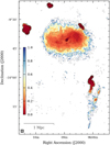 |
Fig. A.1 Spectral index error map of Fig. 10. |
| In the text | |
|
Fig. A.2 Exposure map of the XMM-Newton mosaic of A754. It shows the EPIC net exposure in MOS units. |
| In the text | |
|
Fig. A.3 Map showing the radii of the adaptively binned circular regions. |
| In the text | |
 |
Fig. A.4 Thermodynamic error maps of Fig. 11. |
| In the text | |
Current usage metrics show cumulative count of Article Views (full-text article views including HTML views, PDF and ePub downloads, according to the available data) and Abstracts Views on Vision4Press platform.
Data correspond to usage on the plateform after 2015. The current usage metrics is available 48-96 hours after online publication and is updated daily on week days.
Initial download of the metrics may take a while.