| Issue |
A&A
Volume 690, October 2024
|
|
|---|---|---|
| Article Number | A287 | |
| Number of page(s) | 9 | |
| Section | The Sun and the Heliosphere | |
| DOI | https://doi.org/10.1051/0004-6361/202451279 | |
| Published online | 18 October 2024 | |
Energetic seed particles in self-consistent particle acceleration modeling at interplanetary shock waves
1
Department of Physics and Astronomy, University of Turku, Turku, Finland
2
The Blackett Laboratory, Department of Physics, Imperial College London, London SW7 2AZ, UK
Received:
27
June
2024
Accepted:
17
August
2024
Abstract
Aims. The study investigates the relevance of the seed particle population in the results of particle acceleration in interplanetary shock waves, when wave–particle interactions are treated self-consistently.
Methods. We employed the SOLar Particle Acceleration in Coronal Shocks (SOLPACS) model, which is a proton acceleration simulation in shocks with self-consistent nonlinear wave–particle interactions. We compared a suprathermal monoenergetic injection with a two-component injection, including the suprathermal monoenergetic component and a broad-spectrum energetic component corresponding to the observed background particle spectrum. Energetic particles in the beginning of the simulation could increase the local wave intensities sufficiently to increase the rate of acceleration for injected particles and even reshape the resulting particle energy spectra and spatial distributions. The resulting particle energy spectra, particle spatial distributions, and wave intensity spectra are compared to observations made by Solar Orbiter’s instrument suite of the 2021 October 30 energetic storm particle (ESP) event to evaluate the relevance of the seed particle population in the acceleration model.
Results. The energetic component of the seed particle population shortens the needed acceleration time for particles and enhances the tail of the spectrum to a level that matches the observations. The highest compared energies (> 1 MeV) match only when an energetic component is included in the seed particle population. The wave intensities and spatial distributions, on the other hand, showed no significant differences with the monoenergetic and two-component injection. While the simulated and observed wave intensities match within five minutes before the shock passing, the simulated wave field is too intense farther out from the shock, probably due to a lack of wave damping and/or decay processes in the simulation, leading to particles being slightly overly trapped to regions closer to the shock.
Key words: acceleration of particles / magnetohydrodynamics (MHD) / plasmas / shock waves / turbulence / waves
Corresponding author; This email address is being protected from spambots. You need JavaScript enabled to view it.
© The Authors 2024
 Open Access article, published by EDP Sciences, under the terms of the Creative Commons Attribution License (https://creativecommons.org/licenses/by/4.0), which permits unrestricted use, distribution, and reproduction in any medium, provided the original work is properly cited.
This article is published in open access under the Subscribe to Open model. This email address is being protected from spambots. You need JavaScript enabled to view it. to support open access publication.
1. Introduction
The study of solar energetic particle (SEP) events (see, e.g., Desai & Giacalone 2016) has long been a focal point of research in solar and space physics, driven by their profound implications for both the near-Earth radiation environment (see, e.g., Vainio et al. 2009) and our understanding of particle acceleration in astrophysical objects, such as supernova remnants (see, e.g., Bell 2004) and merging galaxy clusters (see, e.g., van Weeren et al. 2010). SEP events, which involve sporadic and large increases in energetic particle fluxes in the interplanetary medium, are often associated with solar flares and shock waves that propagate through the heliosphere, most often driven by coronal mass ejections (CMEs) (see, e.g., Reames 2023). These shock waves play a pivotal role in particle acceleration of gradual SEP events, yet the intricate mechanisms underlying this phenomenon are understood at a qualitative level only.
Modeling has emerged as a powerful tool to explore and unravel the complexities of particle acceleration in shock waves (see, e.g., Caprioli & Spitkovsky 2014; Ding et al. 2022; Wijsen et al. 2022, 2023; Husidic et al. 2024). In particular, numerical models are valuable for investigating the differential equations governing particle transport and acceleration. A very successful theory to explain particle acceleration at shocks is diffusive shock acceleration (DSA) (Axford et al. 1977; Krymskii 1977; Bell 1978; Blandford & Ostriker 1978). DSA hinges on the interaction between solar wind ions and the turbulent foreshock region generated by the streaming instability (Bell 1978), which has been investigated in several studies (e.g., Lee 1983; Ng & Reames 1994; Gordon et al. 1999; Zank et al. 2000; Vainio 2003; Lee 2005).
Increasing our understanding of SEP acceleration requires delving into the realm of self-consistent modeling. This study employs the particle acceleration and wave generation model SOLar Particle Acceleration in Coronal Shocks (SOLPACS) (Afanasiev et al. 2015). SOLPACS treats wave-particle interactions self-consistently, where both particles and waves are treated as integral components of the same physical system. In this context, the presence of energetic particles is no longer a passive element but actively influences the acceleration process by enhancing wave energy through wave-particle interactions. The interaction between waves and particles results in altered particle acceleration conditions, thereby underscoring the paramount importance of investigating the effects of energetic seed particles for the acceleration of the suprathermal population in self-consistent simulations. Self-consistent models have been studied in several studies (e.g., Bell 1978; Lee 1983, 2005; Gordon et al. 1999; Zank et al. 2000; Vainio & Laitinen 2007; Ng & Reames 2008; Afanasiev et al. 2015; Li et al. 2022). Additionally, self-consistent diffusive approaches have also been investigated (e.g., Berezhko & Taneev 2016; Walter et al. 2022).
SOLPACS offers a means to simulate and investigate the intricate interplay between particles, fluctuations, and shock waves, which is required to investigate the effects of the energetic seed particle population in particle acceleration. In a recent study (Afanasiev et al. 2023) SOLPACS was used to simulate an energetic storm particle (ESP) event. The seed population was assumed to be a suprathermal tail of the particle distribution (exponentially decreasing with the particle speed). However, ESP events are usually observed as superposed on ongoing SEP events (see, e.g., Ameri et al. 2024). Therefore, in this study we investigate what effects the SEP event, which provides an energetic component for the seed particle population, has on the acceleration of suprathermal particles at the shock. Additionally, the turbulence spectra of the SEP event and the spatial distribution of particles upstream of the shock is investigated. ESP events have been investigated with self-consistent DSA models in previous studies (e.g., Berezhko & Taneev 2016; Taneev et al. 2018).
We compared simulation results to observations from Solar Orbiter of the ESP event associated with the 2021 October 28 SEP event. The event has a ground-level enhancement (GLE) associated with it, and hence a great deal of research regarding SEP around it has been done (see, e.g., Mishev et al. 2022; Papaioannou et al. 2022; Kouloumvakos et al. 2024). We present here the relevant observations from the instrument suite on board Solar Orbiter, the particle and wave model SOLPACS, and the results of SOLPACS against the observations, and discuss the implications of the results on our understanding of particle acceleration processes in shock waves.
2. Model and observations
SOLPACS simulates proton acceleration coupled with Alfvén wave generation in the shock upstream with a Monte Carlo model; a sketch highlighting the main features of the model can be seen in Fig. 1. Protons are traced on a single magnetic field line under the guiding center approximation with pitch-angle diffusion and advection modeled. Alfvén waves are traced under the Wentzel-Kramers-Brillouin (WKB) approximation with wave growth taken into account. The model is local (i.e., the plasma and shock parameters are kept constant during the course of the simulation). The model requires the input of five physical parameters: plasma density np, Alfvén speed vA, Alfvénic Mach number in the de Hoffmann–Teller (HT) frame MA, HTF, shock normal angle θBn, and particle injection strength at the shock ϵinj. The last parameter (ϵinj) defines the fraction of particles in the upstream solar wind that participate in the shock acceleration process and is a free parameter, with observations, for example at Earth’s bow shock giving an upper limit of 2.5% (Ellison et al. 1990). There are no energetic particles in the simulation at the start; instead, they are injected over the course of the simulation. A more detailed description of the SOLPACS model can be found in Afanasiev et al. (2015, 2023). The details of the determination of the simulation input parameters are discussed in Appendix A.
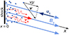 |
Fig. 1. SOLPACS simulation geometry. Protons (blue dots) and their velocity and speed along x (black), Alfvén waves (red), and the upstream plasma flow (dark blue arrow) and the magnetic field (light blue arrows) are depicted in the de Hoffmann–Teller frame, where the shock is at the origin x = 0. The coordinate system has been chosen so that the x-coordinate is along the magnetic field lines. |
To compare the model’s performance to the observations of the ESP event related to the shock observed by Solar Orbiter on 2021 October 30, we employed the observations by Solar Orbiter of the magnetic field by the Magnetometer (MAG) instrument (Horbury et al. 2020), suprathermal ions by the Suprathermal Electrons Protons (STEP) unit of the Energetic Particle Detector (EPD) instrument (Rodríguez-Pacheco et al. 2020), and energetic protons by the Electron Proton Telescope (EPT) unit of the EPD instrument (Rodríguez-Pacheco et al. 2020). The SEP event started at around 16:00 UT on 2021 October 28, and the ESP event is associated with the observed shock arrival at 22:01 UT on 2021 October 30. Particle and magnetic field data approximately two and a half days before the shock associated with the event are presented in Fig. 2.
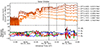 |
Fig. 2. Solar Orbiter/EPT particle data and MAG magnetic field data over several days before the shock arrival at the spacecraft. The shock passing time is denoted by the dashed black line and the background window borders are depicted as solid black lines. |
In this work our aim is to make a more accurate comparison of simulated particle intensities with observations than in Afanasiev et al. (2023), and so we subtracted the background inferred from a selected background time window right before the ESP-associated intensity enhancement (Figs. 2 and 3). The selected background window is highlighted in gray shading in Fig. 3. The background intensities, especially in the higher-energy channels, exhibit an exponentially decaying trend. We estimated the time-dependent background intensities by fitting the time-intensity profiles of each energy channel with a decaying exponential function. We compared the quality of each fit to a constant value (mean of the background window) fit and chose the one with the lowest reduced χ2. In Fig. 3 the intensities close to the shock are shown first without background subtraction (with the best fits overplotted as dashed lines), then with a fixed (constant value) background subtracted, and finally with the time-dependent background subtracted.
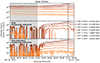 |
Fig. 3. Solar Orbiter/EPT particle data on 2021 October 30. The shock passing the spacecraft is denoted by the dashed black line and the background window used is denoted with a gray box. The top panel shows the original data without background particle intensity considerations (solid lines) and the fitted functions to the temporally evolving background in each energy channel (dashed lines), the middle panel shows a background subtracted data with the mean of the background window as a constant background in each energy channel, and the bottom panel shows a background subtracted data with a temporally evolving background from the fitted functions in the top panel. |
Figure 4 presents a zoomed-in image to two hours before the shock passing of STEP particle data, showing a gradual increase in particle intensities across all energies, MAG magnetic field data, showing a plateau in magnetic field values until right before the shock where a dip in magnetic field magnitude can be seen, and Fourier spectrograms (power spectral densities, PSDs) of the magnetic field data in the three bottom-most panels. The component parallel to the mean magnetic field is B∥ and the two components perpendicular to the mean magnetic field are B⊥1 and B⊥2. The mean magnetic field direction is calculated separately in each time bin (i.e., for each fast Fourier transform, FFT, window) of length 251 s. The FFT windows overlap by 12.5% and we apply a Hann window. For reference, we also plot the proton cyclotron frequency fc, p = eB/(2πmp) and the maximum Doppler-shifted magnetohydrodynamic (MHD) frequency fmax = V/(2πdi). Here, e is the elementary charge, mp is the proton mass, V is the plasma bulk speed, and di is the proton inertial length. We can see that almost all power is located in the MHD regime (below fmax).
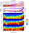 |
Fig. 4. Solar Orbiter’s particle (STEP), magnetic field (MAG), and power spectral densities of magnetic fluctuations acquired by Fourier transforms of the magnetic field data of the energetic storm particle event associated with the 2021 October 28 solar event. The local maximum frequency allowed by MHD, fmax, and the local proton cyclotron frequency, fc, p, are depicted as the white and black lines, respectively. Additionally, three averaging windows to investigate local wave intensity (Fig. 8) are indicated by the black solid line borders and magenta shaded boxes. |
The simulation model has a two-component injection: a combination of a monoenergetic (10 keV) suprathermal population and an energetic injection, where the injection energy spectrum of the seed particles corresponds to a Band function fit, a double power law with a smooth turnover shown in Fig. 5 (Band et al. 1993), to the mean of the observed background intensity window shown in Fig. 2 (for details of the energetic injection, see Appendix B). This provides us with a realistic energetic particle population enhancing the wave population in the simulation to further accelerate the suprathermal proton population. As the simulation results only include particles that have interacted with the shock, to account for the background correctly, we injected half of the background spectrum to the simulation with the energetic injection and subtracted half of the background spectrum from the observational spectrum to account for particles that are in the half of the velocity space that will interact with the shock. We compared the results of this two-component injection to simulation runs with only the monoenergetic suprathermal injection to assess the effect the energetic seed particle population on the simulation results.
Input parameters for solar wind conditions and shock properties were derived from the Solar Orbiter observations with the methods described in Trotta et al. (2022) (see Appendix A) and are listed in Table 1. Additionally, the particle injection strength ϵinj, simulation box size, and initial mean free path of the particles λ0 are listed. The only parameters changed between the monoenergetic and two-component injection case are the particle injection strength at the shock, ϵinj, and the location of the free-escape boundary far upstream of the shock, which implements the simulation box size. A free-escape boundary is not a strictly physical parameter, but can mimic the particle escape caused by adiabatic focusing in the upstream region (e.g., Annie John et al. 2024).
Simulation input parameters for the monoenergetic and two-component injection cases.
3. Results
Particle energy spectra for the monoenergetic injection case can be seen in Fig. 6, where an intermediary simulation snapshot to show the evolution of the simulated particle spectrum and the steady state of the simulation are presented. The background shown in Fig. 5 has been subtracted from the observations. An excellent correspondence between the simulation results in the steady state and the observations can be seen for < 1 MeV particles, while the tail (> 1 MeV) of the simulated spectrum is too soft compared to the observed tail of the spectrum.
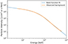 |
Fig. 5. Observed particle intensities of the chosen background as a function of energy and the Band function fit used to sample injection energies and weights of particles that are injected from the energetic domain. |
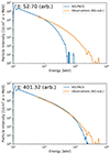 |
Fig. 6. Particle energy spectra of the SOLPACS simulation results for the monoenergetic injection case with a particle injection energy of 10 keV and observational data from Solar Orbiter/EPT. The background particle intensity shown in Fig. 5 has been subtracted from the observational data. The time of the simulation snapshot is shown in arbitrary units at the top. The top panel shows an intermediate snapshot of simulation progress, where the particles have not yet had the time to be accelerated to high enough energies to match the observations. The bottom panel shows the simulation steady state, where close correspondence to the observations can be seen. |
Particle energy spectra for the two-component injection case can be seen in Fig. 7 in the same format as for the monoenergetic injection case in Fig. 6. Because the simulation results only include particles that have interacted with the shock, only half of the background intensity is subtracted to account for the particles that have not yet interacted with the shock. A similarly excellent correspondence between the simulation steady state and the observations is seen, but now with less in-simulation (acceleration) time needed. In addition, the model now reproduces the high-energy tail of the distribution much better than the monoenergetic injection case.
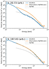 |
Fig. 7. Particle energy spectra of the SOLPACS simulation results for the two-component injection case with suprathermal protons being injected at 10 keV and energetic protons being sampled from the Band function shown in Fig. 5, and the observational data from Solar Orbiter/EPT. Half of the temporally evolved background particle intensity (dotted black line) has been subtracted from the observational data to account for the background particles that have not yet reached the shock. The time of the simulation snapshot is shown in arbitrary units at the top. The top panel shows an intermediate snapshot of simulation progress, where the particles have not yet had the time to be accelerated to high enough energies to match the observations. The bottom panel shows the simulation steady state, where close correspondence to the observations can be seen. |
We now go beyond the comparison between observed and simulated spectra, and address the wave generation in the shock upstream, which is possible thanks to the self-consistency of our model. The wave intensity as a function of frequency can be compared to the PSD of observed magnetic field data shown in Fig. 4. We compare the wave intensity of the left- and right-handed polarization modes as a function of frequency at the three different averaging windows in Fig. 4 as a comparison between simulations and observations. The intensity of the right- and left-handed polarized waves in the observations are estimated by applying the FFT on B⊥1 + iB⊥2 and B⊥1 − iB⊥2, respectively, and considering the power in positive frequencies. Due to the nonlinearity of the model, the initial spectrum is not very significant as the self-generated waves dominate in the steady state of the simulation. The comparison for the two-component injection case can be seen in Fig. 8, where a good match between the simulated and observed wave spectra can be seen close to the shock (panel 3). The solar wind speed used (usw = 325 km/s) to solve for frequency from the wave number was checked from the Solar Orbiter quick-look plots of the Swedish Institute of Space Physics (IRF)1. Farther away from the shock we see more intense wave spectra in the simulated results compared to the observed ones. This is possibly due to the assumption of homogeneity in the simulation model, becoming less justified when looking at long time (spatial) scales upstream of the shock. The result of the monoenergetic injection case is practically identical to the two-component case, and so it is omitted.
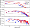 |
Fig. 8. Left- and right-handed polarization mode wave intensity as a function of wave frequency for the two-component injection SOLPACS case (colored dashed lines), the seed wave population of SOLPACS (gray dashed line), and the fast Fourier transform (FFT) wave spectra of the observations made by Solar Orbiter/MAG (solid colored lines). The wave intensity in plots 1–3 correspond to the mean over the similarly indexed boxes in Fig. 4. The result for the monoenergetic injection case is practically identical to the two-component case, and so was omitted. |
One can also look at the spatial distribution of the particles to see if the injection, particle trapping to the vicinity of the shock, and escape conditions correspond to the observations. We applied Taylor’s hypothesis (Taylor 1938) to derive the spatial distributions from the particle time series data measured by Solar Orbiter,
 (1)
(1)
where vs/c is the spacecraft speed in the shock frame along the mean magnetic field
 (2)
(2)
x is the distance from the shock corresponding to the temporal distance from the shock, tsh is the time of arrival of the shock at the spacecraft, t is the time stamp of each data point being translated, vsh is the shock speed in the spacecraft frame along the shock normal, and θBn is the shock obliquity.
The spatial distribution of the monoenergetic injection case can be seen in Fig. 9, where a good correspondence can be seen between the simulation results and observations, although far from the shock the temporally evolving background particle intensity exceeds the observational values. The spatial distribution of the two-component injection case can be seen in Fig. 10, where, again, a reasonably good correspondence can be seen between the simulation results and observations, with the background subtraction not causing any values below zero as only half of the background is again accounted for as for the particle energy spectra results in Fig. 7.
 |
Fig. 9. Spatial distribution of particle intensity of observations made by Solar Orbiter/EPT, where the timing of particle intensity measurements has been translated to position following Eq. (1), and simulation results for the monoenergetic injection case of SOLPACS. |
4. Discussion
The SOLPACS simulation model reproduces the bulk particle spectrum of the ESP event with great accuracy in both injection implementations, with the two-component injection nicely reproducing the high-energy tail that forms the broken power law spectrum seen in the observations. The derived gas compression ratio of the shock can be used to predict the spectral index of the particle energy spectrum. Solving the gas compression ratio from the input parameters of the simulations ( , θBn = 56°, β = 0.378, see Fig. A.1) results in rg = 2.931, and furthermore a spectral index qobs = −1.540, which corresponds closely to estimates of the slopes in both injection cases, qsim ≈ −1.5.
As the monoenergetic and the two-component injection case both result in very good correspondence with observations of energetic particles at the shock, we can make two interpretations of the particle acceleration situation. The monoenergetic case would correspond to a situation where we are simply looking at the particles that the shock accelerates without any other factors taken into account, as the background is completely subtracted from the observations. In the two-component injection case, a high particle energy background is considered, which can be interpreted as resulting from a previous particle acceleration event, for example (the GLE in the present case).
The simulation generated wave spectra suggest that the simulation seems to be missing a damping process that leaves an intense tail to the wave spectrum at higher frequencies in Fig. 8. Such high-frequency damping could be related to the damping caused by thermal and mildly suprathermal ions that are part of the upstream solar wind plasma. Additionally, the PSD of the magnetic field data contains other wave modes than Alfvèn waves, leading to the observational wave spectrum being even less intense than currently depicted when limited only to Alfvén waves, though this does not change our conclusion that SOLPACS generates more waves than observed. Wave decay by wave–wave interactions (see, e.g., Nyberg & Vainio 2022) can also decrease the intensity of the Alfvén waves.
As the wave spectra of the simulation results are more intense than the FFT of the observations gives, the correspondence in the spatial distributions of particles in the lowest energy channel (50–100 keV) in Figs. 9 and 10 indicate that the intense wave spectrum is consistent with a more confined particle distribution. In particular, the two-component injection case would correspond better with the observations with an increased mean free path (i.e., reduced wave intensity) to allow the protons to escape farther from the shock.
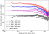 |
Fig. 10. Spatial distribution of particle intensity of observations made by Solar Orbiter/EPT, where the timing of particle intensity measurements has been translated to position following Eq. (1), and simulation results for the two-component injection case of SOLPACS. |
To reach a physical steady state in particle acceleration modeling, adiabatic focusing (Roelof 1969) must be accounted for (see, e.g., Annie John et al. 2024). As SOLPACS is a local model, where the global non-uniform structure of the magnetic field cannot be accounted for, focusing is not implemented, and as such the simulation cannot reach a steady state without taking additional measures. To reach a steady state, a finite simulation box with a free-escape boundary can be used to mimic focusing and reach a steady state, as depicted in Fig. 11. As focusing allows the particle to escape from the shock front, a free-escape boundary similarly allows a particle to escape the shock front by leaving the simulation box, resulting in the removal of the particle from the simulation. The connection between focusing length (see, e.g., Vainio et al. 2000) and simulation box size has recently been investigated in more detail in Annie John et al. (2024).
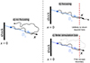 |
Fig. 11. Different cases of particle transport conditions are depicted in the three settings above: a) Without focusing, depicting a particle scattering back to the shock after traveling far from it; b) With focusing, depicting a particle escaping the shock as focusing pushes it away from the shock; c) With a finite simulation box, depicting a particle escaping the shock similarly to the focusing-included case, as particles are not able to return beyond the free-escape boundary of the simulation box. |
With the presence of energetic particles in the simulation, a smaller box size in the two-component injection case compared to the monoenergetic injection case is used to gain a better correspondence to the simulations. With a larger box size a larger population of > MeV particles would be present in the steady state of the simulation, without the cutoff energy significantly increasing, leading simply to a harder spectrum with enough time. In this regard, a larger box size will not improve the resultant particle energy spectrum of the monoenergetic injection case seen in Fig. 6.
Physical shocks are not as simple as MHD-based models assume them to be, but rather contain large-scale evolution and small local structures, which manifest as different acceleration conditions for different flux tubes. These kinds of shock structures have been studied in the context of irregular particle injection to suprathermal energies in Trotta et al. (2023) and in the context of reflected particles and their interplay with shock microstructuring in Dimmock et al. (2023). Looking at the particle data presented in Figs. 4 and A.1, one can see that the data is not consistent with simple constant shock parameters or a single flux tube, presenting the issue in shock acceleration modeling and shock evolution characterization.
5. Conclusions and outlook
The presented work furthers our knowledge of several aspects of particle acceleration at shocks and its interplay with self-generated fluctuations. Wave intensity spectra of self-consistently simulated wave–particle interactions were compared to observed wave intensity spectra, demonstrating good correspondence close to the shock and highlighting the need for additional wave evolution processes to account for the spectra far from the shock. Additionally, the model requires only two free parameters to perfectly match the simulated spectrum to the observed one with the two-component injection, greatly contributing to our understanding and realistic modeling of particle acceleration processes in shock waves.
The results for including energetic particles in the injection population of particles in self-consistent models are highly promising. The shorter in-simulation time needed to achieve a steady state and the excellent reproduction of the high-energy tail of the observations indicate a significant step closer to realistic numerical particle acceleration simulations. High-energy particles have been modeled with close correspondence to the observations using more global shock parameters, as the larger-scale shock properties align better with larger acceleration timescales.
The wave intensity spectra suggest that with some additional efforts, the modeling of waves far from the shock can be further improved. The presented intense wave spectra might result from the local nature of the simulation model or from a damping or a decay process that has not yet been implemented. Furthermore, the spatial distributions indicate that the wave intensities are slightly too high, leading to some excess particle trapping closer to the shock.
The relevance of self-consistent wave–particle interactions in particle acceleration modeling cannot be overstated. These interactions are fundamental to understanding how particles gain energy in shock environments. SOLPACS stands out as an excellent model for particle acceleration in interplanetary shock waves by incorporating self-consistent wave–particle interactions with only two free parameters. The model ensures that the feedback between particles and waves is accurately represented, providing deeper insights into the mechanisms driving particle acceleration and enabling more precise predictions and interpretations of observational data.
Acknowledgments
Funded by the European Union. Views and opinions expressed are however those of the authors only and do not necessarily reflect those of the European Union or HaDEA. Neither the European Union nor the granting authority can be held responsible for them. This research has received funding from the European Union’s Horizon 2020 research and innovation programme under grant agreement No. 101004159 (SERPENTINE) and from the Finnish Cultural Foundation, Varsinais-Suomi Regional fund. The computer resources of the Finnish IT Center for Science (CSC) and the FGCI project (Finland) are acknowledged. LV acknowledges the financial support of the University of Turku Graduate School. The work in the University of Turku is performed under the umbrella of Finnish Centre of Excellence in Research of Sustainable Space (FORESAIL).
References
- Afanasiev, A., Battarbee, M., & Vainio, R. 2015, A&A, 584, A81 [NASA ADS] [CrossRef] [EDP Sciences] [Google Scholar]
- Afanasiev, A., Vainio, R., Trotta, D., et al. 2023, A&A, 679, A111 [CrossRef] [EDP Sciences] [Google Scholar]
- Ameri, D., Vainio, R., & Valtonen, E. 2024, Adv. Space Res., 73, 1050 [NASA ADS] [CrossRef] [Google Scholar]
- Annie John, L., Nyberg, S., Vuorinen, L., et al. 2024, J. Space Weather Space Clim., 14, 15 [NASA ADS] [CrossRef] [EDP Sciences] [Google Scholar]
- Axford, W. I., Leer, E., & Skadron, G. 1977, Int. Cosmic Ray Conf., 11, 132 [Google Scholar]
- Band, D., Matteson, J., Ford, L., et al. 1993, ApJ, 413, 281 [Google Scholar]
- Bell, A. R. 1978, MNRAS, 182, 147 [Google Scholar]
- Bell, A. R. 2004, MNRAS, 353, 550 [Google Scholar]
- Berezhko, E. G., & Taneev, S. N. 2016, Astron. Lett., 42, 126 [CrossRef] [Google Scholar]
- Blandford, R. D., & Ostriker, J. P. 1978, ApJ, 221, L29 [Google Scholar]
- Caprioli, D., & Spitkovsky, A. 2014, ApJ, 783, 91 [CrossRef] [Google Scholar]
- Desai, M., & Giacalone, J. 2016, Liv. Rev. Sol. Phys., 13, 3 [NASA ADS] [CrossRef] [Google Scholar]
- Dimmock, A. P., Gedalin, M., Lalti, A., et al. 2023, A&A, 679, A106 [NASA ADS] [CrossRef] [EDP Sciences] [Google Scholar]
- Ding, Z., Wijsen, N., Li, G., & Poedts, S. 2022, A&A, 668, A71 [NASA ADS] [CrossRef] [EDP Sciences] [Google Scholar]
- Ellison, D. C., Moebius, E., & Paschmann, G. 1990, ApJ, 352, 376 [CrossRef] [Google Scholar]
- Gordon, B. E., Lee, M. A., Möbius, E., & Trattner, K. J. 1999, J. Geophys. Res., 104, 28263 [NASA ADS] [CrossRef] [Google Scholar]
- Horbury, T. S., O’Brien, H., Carrasco Blazquez, I., et al. 2020, A&A, 642, A9 [NASA ADS] [CrossRef] [EDP Sciences] [Google Scholar]
- Husidic, E., Wijsen, N., Baratashvili, T., Poedts, S., & Vainio, R. 2024, J. Space Weather Space Clim., 14, 11 [NASA ADS] [CrossRef] [EDP Sciences] [Google Scholar]
- Kouloumvakos, A., Papaioannou, A., Waterfall, C. O. G., et al. 2024, A&A, 682, A106 [NASA ADS] [CrossRef] [EDP Sciences] [Google Scholar]
- Krymskii, G. F. 1977, Akademiia Nauk SSSR Doklady, 234, 1306 [NASA ADS] [Google Scholar]
- Lee, M. A. 1983, J. Geophys. Res., 88, 6109 [NASA ADS] [CrossRef] [Google Scholar]
- Lee, M. A. 2005, ApJS, 158, 38 [NASA ADS] [CrossRef] [Google Scholar]
- Li, G., Bruno, A., Lee, M. A., et al. 2022, ApJ, 936, 91 [NASA ADS] [CrossRef] [Google Scholar]
- Mishev, A. L., Kocharov, L. G., Koldobskiy, S. A., et al. 2022, Sol. Phys., 297, 88 [NASA ADS] [CrossRef] [Google Scholar]
- Ng, C. K., & Reames, D. V. 1994, ApJ, 424, 1032 [NASA ADS] [CrossRef] [Google Scholar]
- Ng, C. K., & Reames, D. V. 2008, ApJ, 686, L123 [NASA ADS] [CrossRef] [Google Scholar]
- Nyberg, S., & Vainio, R. 2022, Physics, 4, 394 [NASA ADS] [CrossRef] [Google Scholar]
- Owen, C. J., Bruno, R., Livi, S., et al. 2020, A&A, 642, A16 [EDP Sciences] [Google Scholar]
- Papaioannou, A., Kouloumvakos, A., Mishev, A., et al. 2022, A&A, 660, L5 [NASA ADS] [CrossRef] [EDP Sciences] [Google Scholar]
- Reames, D. V. 2023, Space Sci. Rev., 219, 14 [NASA ADS] [CrossRef] [Google Scholar]
- Rodríguez-Pacheco, J., Wimmer-Schweingruber, R. F., Mason, G. M., et al. 2020, A&A, 642, A7 [Google Scholar]
- Roelof, E. C. 1969, in Lectures in High-Energy Astrophysics, eds. H. Ögelman, & J. R. Wayland, 111 [Google Scholar]
- Taneev, S. N., Starodubtsev, S. A., & Berezhko, E. G. 2018, Sov. J. Exp. Theor. Phys., 126, 636 [NASA ADS] [CrossRef] [Google Scholar]
- Taylor, G. I. 1938, Proc. R. Soc. London Ser. A, 164, 476 [Google Scholar]
- Trotta, D., Vuorinen, L., Hietala, H., et al. 2022, Front. Astron. Space Sc., 9, 1005672 [NASA ADS] [CrossRef] [Google Scholar]
- Trotta, D., Horbury, T. S., Lario, D., et al. 2023, ApJ, 957, L13 [CrossRef] [Google Scholar]
- Vainio, R. 2003, A&A, 406, 735 [NASA ADS] [CrossRef] [EDP Sciences] [Google Scholar]
- Vainio, R., & Laitinen, T. 2007, ApJ, 658, 622 [NASA ADS] [CrossRef] [Google Scholar]
- Vainio, R., Kocharov, L., & Laitinen, T. 2000, ApJ, 528, 1015 [CrossRef] [Google Scholar]
- Vainio, R., Desorgher, L., Heynderickx, D., et al. 2009, Space Sci. Rev., 147, 187 [Google Scholar]
- van Weeren, R. J., Röttgering, H. J. A., Brüggen, M., & Hoeft, M. 2010, Science, 330, 347 [Google Scholar]
- Walter, D., Effenberger, F., Fichtner, H., & Litvinenko, Y. 2022, Phys. Plasmas, 29, 072302 [NASA ADS] [CrossRef] [Google Scholar]
- Wijsen, N., Aran, A., Scolini, C., et al. 2022, A&A, 659, A187 [NASA ADS] [CrossRef] [EDP Sciences] [Google Scholar]
- Wijsen, N., Lario, D., Sánchez-Cano, B., et al. 2023, ApJ, 950, 172 [NASA ADS] [CrossRef] [Google Scholar]
- Zank, G. P., Rice, W. K. M., & Wu, C. C. 2000, J. Geophys. Res., 105, 25079 [NASA ADS] [CrossRef] [Google Scholar]
Appendix A: Shock wave parameter investigation
The choice of the windows for evaluating the shock properties from the observations becomes a topic of discussion when deciding on what particle populations are of interest in the modeling task. As higher-energy particles require more time to be accelerated, more global, larger scale shock properties should be considered. With lower-energy particles, acceleration times are shorter, and as such, more local and smaller scale shock properties are of interest. Looking at the observational data close to the shock (Figs. 4 and A.1) one can see significantly different structures with small scales very close to the shock compared to the larger structures farther away from the shock.
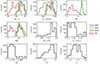 |
Fig. A.1. Shock parameter distributions of the different windows of Fig. A.2. For applicable values, the mixed mode and co-planar values are shown separately. |
The shock parameters are selected based on an observational analysis of the shock crossing, using Solar Orbiter MAG (Horbury et al. 2020) and SWA (Owen et al. 2020) measurements (Fig. A.2). As in Trotta et al. (2022), a large averaging window (lighter blue and red) is chosen from which smaller windows of increasing size (darker blue and red) are formed (Fig. A.2). The distributions of average plasma and shock properties from the averaging windows are then plotted. As we are interested in acceleration of high-energy particles, windows farther away from the shock are chosen to represent a more global shock structure, as high-energy particles need several hours to be accelerated.
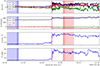 |
Fig. A.2. Zoomed-in image on a roughly 30 min window around the shock passing of SWA plasma data and MAG magnetic field data. The lighter blue window upstream of the shock shows the largest averaging window for the shock parameters, while the darker blue shows the smallest window. The red boxes on the downstream side correspondingly show the same things. |
Appendix B: Details of the two-component injection
Instead of a monoenergetic injection as for the suprathermal component of the two-component injection, a spectrum of particle energies needs to be injected for the energetic component. In addition to the particle energy Einj, ener needing to be sampled for the injection, the particle’s weight in the simulation w needs to be sampled correspondingly to ensure that wave growth due to self-consistent wave–particle interactions is modeled correctly. The monoenergetic and energetic seed particles have an initial physical normalization weight wphys = ϵinjnputmax, where ϵinj is the particle injection strength at the shock, np the particle density, u the upstream flow speed in the shock frame along the mean magnetic field, and tmax the maximum simulation time set, before the adjustments mentioned in this Appendix are made.
The energetic particle energies are sampled from a Band function fit (Eq. (B.1) (Band et al. 1993)) to the observed background intensities. The background intensity is defined as the mean of the window of observed particle intensities in Fig. 2 as a function of energy (Fig. 5). The Band function is a double power law with a smooth turnover:
![Mathematical equation: $$ \begin{aligned} f(E) = \left\{ \begin{array}{l} kE^{\gamma _\mathrm{1} } \mathrm{e} ^{-\frac{E}{E_\mathrm{C} }} ,\ E < (\gamma _\mathrm{1} -\gamma _\mathrm{2} )E_\mathrm{C} \\ kE^{\gamma _\mathrm{2} } \left[ \left(\gamma _\mathrm{1} -\gamma _\mathrm{2} \right) E_\mathrm{C} \mathrm{e} ^{-1}\right]^{\gamma _\mathrm{1} -\gamma _\mathrm{2} } ,\ E \ge (\gamma _\mathrm{1} -\gamma _\mathrm{2} )E_\mathrm{C} . \end{array}\right. \end{aligned} $$](/articles/aa/full_html/2024/10/aa51279-24/aa51279-24-eq4.gif) (B.1)
(B.1)
The fit is done in a relevant energy range from E0 = 10 keV to E1 = 5000 keV to investigate the role of abundant high-energy particles. The acquired fit parameters are EC = 407 keV, γ1 = −0.335, γ2 = −2.67, and k = 13600 cm−2 sr−1 s−1 MeV−1 − γ1.
The fitted Band function is normalized to resemble the realistic portion of energetic particles participating in the acceleration process in the observations by adjusting the weight of each Monte Carlo particle. To adjust the weight of particles between the monoenergetic and energetic injection domains correctly, we use the observed particle density and particle injection strength. The observed density of all particles participating in the acceleration process is simply the observed density of particles  multiplied by the particle injection strength ϵinj = 1.6 ⋅ 10−4,
 (B.2)
(B.2)
To determine the probability of injecting a Monte Carlo particle in the energetic component rather than the monoenergetic component so that the seed population can be considered realistic, the energetic seed particle density is calculated in the nonrelativistic regime as
 (B.3)
(B.3)
 (B.4)
(B.4)
resulting in a density of energetic injection component particles participating in the acceleration process of
 (B.5)
(B.5)
with the portion of energetic component particles of all injected particles being
 (B.6)
(B.6)
If the Monte Carlo particle is chosen to be injected in the energetic domain, its energy is sampled from an exponential function and its weight is adjusted according the Band function to avoid having “bombs”: singular high-energy particles, that could cause instabilities in the wave spectra through self-consistent wave growth. The exponential function from which the particle energies are sampled is
 (B.7)
(B.7)
 (B.8)
(B.8)
where E0 = 10 keV, E1 = 5000 keV, and R is a random number between 0 and 1 (including 0). The weight factor wf is solved from a function form similar to Eq. (B.1):
![Mathematical equation: $$ \begin{aligned} w_{\rm f}(E_\mathrm{inj,ener} ) = \left\{ \begin{array}{l} \left(\frac{E_\mathrm{inj,ener} }{E_1}\right)^{\gamma _\mathrm{1} +1} \mathrm{e} ^{-E_\mathrm{inj,ener} /E_\mathrm{C} } ,\ E_\mathrm{inj,ener} < (\gamma _\mathrm{1} -\gamma _\mathrm{2} )E_\mathrm{C} \\ \left(\frac{E_\mathrm{inj,ener} }{E_1}\right)^{\gamma _\mathrm{2} +1} \left[ \left(\gamma _\mathrm{1} -\gamma _\mathrm{2} \right) \frac{E_\mathrm{C} }{E_1}\right]^{\gamma _\mathrm{1} -\gamma _\mathrm{2} } \mathrm{e} ^{\gamma _\mathrm{2} -\gamma _\mathrm{1} } ,\ E_\mathrm{inj,ener} \ge (\gamma _\mathrm{1} -\gamma _\mathrm{2} )E_\mathrm{C} . \end{array}\right. \end{aligned} $$](/articles/aa/full_html/2024/10/aa51279-24/aa51279-24-eq13.gif) (B.9)
(B.9)
In order to account for the wave growth resulting from the self-consistent wave–particle interactions correctly, the weight factor wf is normalized with a factor C so that its average for Monte Carlo particles injected in the energetic domain is ⟨wf⟩ = 1:
 (B.10)
Using the Band function and its respective limits results in an inverse weight normalization factor of
![Mathematical equation: $$ \begin{aligned} \begin{aligned} \Rightarrow C^{-1} =&\frac{\int _{E_\mathrm{0} }^{(\gamma _\mathrm{1} -\gamma _\mathrm{2} )E_\mathrm{C} } \left(\frac{E}{E_\mathrm{0} }\right)^{\gamma _\mathrm{1} +1} \mathrm{e} ^{-E/E_\mathrm{C} } \mathrm{d} E}{(\gamma _\mathrm{1} -\gamma _\mathrm{2} )E_\mathrm{C} - E_\mathrm{0} } \\ +&\frac{\int _{(\gamma _\mathrm{1} -\gamma _\mathrm{2} )E_\mathrm{C} }^{E_\mathrm{1} } \left(\frac{E}{E_\mathrm{0} }\right)^{\gamma _\mathrm{2} +1} \left[\left(\gamma _\mathrm{1} -\gamma _\mathrm{2} \right) E_\mathrm{C} E_\mathrm{0} ^{-1}\mathrm{e} ^{-1}\right] \mathrm{d} E}{E_\mathrm{1} -(\gamma _\mathrm{1} -\gamma _\mathrm{2} )E_\mathrm{C} } , \end{aligned} \end{aligned} $$](/articles/aa/full_html/2024/10/aa51279-24/aa51279-24-eq15.gif) (B.11)
(B.11)
from which we can solve for the physical normalization factor C of the energetic seed particles to be C ≈ 0.252 for the aforementioned Band function fit.
To use the Monte Carlo particles more efficiently in order to cut down the processing time of the simulations, the statistical relevance of the energetic component is enhanced by adjusting the amount of energetic particles injected to half of all Monte Carlo particles injected, and, in turn, adjusting the weight of the energetic component particles smaller and the weight of the monoenergetic component particles larger,
 (B.12)
 (B.13)
resulting in population weight factors of Cnew, mono = 1.783 and Cnew, ener = 0.217 for the Band function fit. Finally, the resulting weight for monoenergetic seed particles is
 (B.14)
and for energetic particles
 (B.15)
To summarize, if a particle is injected in the monoenergetic domain (probability of this injection is 50 %), it’s energy is simply set as Einj = 10 keV and the particle’s weight is according to Eq. (B.14). If a particle is injected in the energetic domain (probability of this injection is also 50 %), it’s energy is sampled from Eq. (B.8) and it’s weight is according to Eq. (B.15).
All Tables
Simulation input parameters for the monoenergetic and two-component injection cases.
All Figures
|
Fig. 1. SOLPACS simulation geometry. Protons (blue dots) and their velocity and speed along x (black), Alfvén waves (red), and the upstream plasma flow (dark blue arrow) and the magnetic field (light blue arrows) are depicted in the de Hoffmann–Teller frame, where the shock is at the origin x = 0. The coordinate system has been chosen so that the x-coordinate is along the magnetic field lines. |
| In the text | |
|
Fig. 2. Solar Orbiter/EPT particle data and MAG magnetic field data over several days before the shock arrival at the spacecraft. The shock passing time is denoted by the dashed black line and the background window borders are depicted as solid black lines. |
| In the text | |
|
Fig. 3. Solar Orbiter/EPT particle data on 2021 October 30. The shock passing the spacecraft is denoted by the dashed black line and the background window used is denoted with a gray box. The top panel shows the original data without background particle intensity considerations (solid lines) and the fitted functions to the temporally evolving background in each energy channel (dashed lines), the middle panel shows a background subtracted data with the mean of the background window as a constant background in each energy channel, and the bottom panel shows a background subtracted data with a temporally evolving background from the fitted functions in the top panel. |
| In the text | |
|
Fig. 4. Solar Orbiter’s particle (STEP), magnetic field (MAG), and power spectral densities of magnetic fluctuations acquired by Fourier transforms of the magnetic field data of the energetic storm particle event associated with the 2021 October 28 solar event. The local maximum frequency allowed by MHD, fmax, and the local proton cyclotron frequency, fc, p, are depicted as the white and black lines, respectively. Additionally, three averaging windows to investigate local wave intensity (Fig. 8) are indicated by the black solid line borders and magenta shaded boxes. |
| In the text | |
|
Fig. 5. Observed particle intensities of the chosen background as a function of energy and the Band function fit used to sample injection energies and weights of particles that are injected from the energetic domain. |
| In the text | |
|
Fig. 6. Particle energy spectra of the SOLPACS simulation results for the monoenergetic injection case with a particle injection energy of 10 keV and observational data from Solar Orbiter/EPT. The background particle intensity shown in Fig. 5 has been subtracted from the observational data. The time of the simulation snapshot is shown in arbitrary units at the top. The top panel shows an intermediate snapshot of simulation progress, where the particles have not yet had the time to be accelerated to high enough energies to match the observations. The bottom panel shows the simulation steady state, where close correspondence to the observations can be seen. |
| In the text | |
|
Fig. 7. Particle energy spectra of the SOLPACS simulation results for the two-component injection case with suprathermal protons being injected at 10 keV and energetic protons being sampled from the Band function shown in Fig. 5, and the observational data from Solar Orbiter/EPT. Half of the temporally evolved background particle intensity (dotted black line) has been subtracted from the observational data to account for the background particles that have not yet reached the shock. The time of the simulation snapshot is shown in arbitrary units at the top. The top panel shows an intermediate snapshot of simulation progress, where the particles have not yet had the time to be accelerated to high enough energies to match the observations. The bottom panel shows the simulation steady state, where close correspondence to the observations can be seen. |
| In the text | |
|
Fig. 8. Left- and right-handed polarization mode wave intensity as a function of wave frequency for the two-component injection SOLPACS case (colored dashed lines), the seed wave population of SOLPACS (gray dashed line), and the fast Fourier transform (FFT) wave spectra of the observations made by Solar Orbiter/MAG (solid colored lines). The wave intensity in plots 1–3 correspond to the mean over the similarly indexed boxes in Fig. 4. The result for the monoenergetic injection case is practically identical to the two-component case, and so was omitted. |
| In the text | |
|
Fig. 9. Spatial distribution of particle intensity of observations made by Solar Orbiter/EPT, where the timing of particle intensity measurements has been translated to position following Eq. (1), and simulation results for the monoenergetic injection case of SOLPACS. |
| In the text | |
|
Fig. 10. Spatial distribution of particle intensity of observations made by Solar Orbiter/EPT, where the timing of particle intensity measurements has been translated to position following Eq. (1), and simulation results for the two-component injection case of SOLPACS. |
| In the text | |
|
Fig. 11. Different cases of particle transport conditions are depicted in the three settings above: a) Without focusing, depicting a particle scattering back to the shock after traveling far from it; b) With focusing, depicting a particle escaping the shock as focusing pushes it away from the shock; c) With a finite simulation box, depicting a particle escaping the shock similarly to the focusing-included case, as particles are not able to return beyond the free-escape boundary of the simulation box. |
| In the text | |
|
Fig. A.1. Shock parameter distributions of the different windows of Fig. A.2. For applicable values, the mixed mode and co-planar values are shown separately. |
| In the text | |
|
Fig. A.2. Zoomed-in image on a roughly 30 min window around the shock passing of SWA plasma data and MAG magnetic field data. The lighter blue window upstream of the shock shows the largest averaging window for the shock parameters, while the darker blue shows the smallest window. The red boxes on the downstream side correspondingly show the same things. |
| In the text | |
Current usage metrics show cumulative count of Article Views (full-text article views including HTML views, PDF and ePub downloads, according to the available data) and Abstracts Views on Vision4Press platform.
Data correspond to usage on the plateform after 2015. The current usage metrics is available 48-96 hours after online publication and is updated daily on week days.
Initial download of the metrics may take a while.