| Issue |
A&A
Volume 690, October 2024
|
|
|---|---|---|
| Article Number | L6 | |
| Number of page(s) | 8 | |
| Section | Letters to the Editor | |
| DOI | https://doi.org/10.1051/0004-6361/202451134 | |
| Published online | 09 October 2024 | |
Letter to the Editor
Origin of the type III radiation observed near the Sun
1
Space Sciences Laboratory, University of California, Berkeley, California, USA
2
Physics Department, University of California, Berkeley, California, USA
3
University of Minnesota, Minneapolis, Minnesota, USA
4
LPC2E, CNRS-University of Orléans-CNES, 45071 Orléans, France
5
Max-Planck Institute of Solar System Research, Göttingen, Germany
6
Uzhhorod National University, Uzhhorod, Ukraine
Received:
15
June
2024
Accepted:
6
September
2024
Aims. We investigate processes associated with the generation of type III radiation using Parker Solar Probe measurements.
Methods. We measured the amplitudes and phase velocities of electric and magnetic fields and their associated plasma density fluctuations.
Results. 1. There are slow electrostatic waves near the Langmuir frequency and at as many as six harmonics, the number of which increases with the amplitude of the Langmuir wave. Their electrostatic nature is shown by measurements of the plasma density fluctuations. From these density fluctuations and the electric field magnitude, the k-value of the Langmuir wave is estimated to be 0.14 and kλd = 0.4. Even with the large uncertainty in this quantity (more than a factor of two), the phase velocity of the Langmuir wave was < 10 000 km/s. 2. The electromagnetic wave near the Langmuir frequency has a phase velocity lower than 50 000 km/s. 3. We cannot determine whether there are electromagnetic waves at the harmonics of the Langmuir frequency. If they existed, their magnetic field components would be below the noise level of the measurement. 4. The rapid (less than one millisecond) amplitude variations typical of the Langmuir wave and its harmonics are artifacts resulting from the addition of two waves, one of which has small frequency variations that arise because the wave travels through density irregularities. None of these results are expected in or consistent with the conventional model of the three-wave interaction of two counter-streaming Langmuir waves that coalesce to produce the type III wave. They are consistent with a new model in which electrostatic antenna waves are produced at the harmonics by radiation of the Langmuir wave, after which at least the first harmonic wave evolved through density irregularities such that its wave number decreased and it became the type III radiation.
Key words: Sun: radio radiation / solar wind
© The Authors 2024
 Open Access article, published by EDP Sciences, under the terms of the Creative Commons Attribution License (https://creativecommons.org/licenses/by/4.0), which permits unrestricted use, distribution, and reproduction in any medium, provided the original work is properly cited.
This article is published in open access under the Subscribe to Open model. Subscribe to A&A to support open access publication.
1. Introduction
An important wave near the Sun is type III radiation, which is an electromagnetic wave whose frequency decreases with time and distance from the Sun. The theory of type III bursts was described by Ginzburg & Zheleznyakov (1958) as a multistep process in which Langmuir waves are produced by an electron beam, after which some of these waves interact with density irregularities to become backward waves that coalesce with the forward waves in a three-wave process that produces the electromagnetic type III radiation. The theory was subsequently discussed and refined by many authors (e.g., Sturrock 1964; Zheleznyakov & Zaitsev 1970; Smith 1970; Smith et al. 1976; Goldman et al. 1980; Dulk 1985; Melrose 1987). The first in situ spectral observations of plasma waves in association with type III emissions were made by Gurnett & Anderson (1976). Their simultaneous observation of Langmuir waves, harmonic electric field emissions, and electromagnetic waves was presented as evidence of the direct conversion of pairs of Langmuir waves into type III waves, although the direct in situ evidence of this interaction was not and has not been obtained.
2. Data
On March 21, 2023, the Parker Solar Probe was located about 45 solar radii from the Sun when it became embedded in the active type III emission region illustrated in Figure 1a. The colored lines below the emission (at the plasma frequency) indicate times when large electric fields appeared. The type III emission covered the frequency range from about 200 to 400 kHz at the time of about 26 bursts of high-rate data illustrated in Figure 1b. These bursts each consisted of ∼15 milliseconds of electric and magnetic field measurements at a data rate of about 1.9 million samples/second (Bale et al. 2016). That the emission range covered more than just twice the plasma frequency was noted earlier (Kellogg 1980; Reiner & MacDowall 2019; Jebaraj et al. 2023), and this aspect of the emission is investigated below.
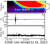 |
Fig. 1. Overview of the type III emission observed on March 21, 2023 (panel a) in which the spacecraft was embedded, showing bright lines below the emission due to large electric fields. The plasma frequency of 125 kHz in panel c shows that these bright lines were due to waves at or near the plasma frequency. These waves are present only part of the time. Panel b shows the times and electric field amplitudes of 26 data bursts taken for durations of about 15 milliseconds each at data rates in excess of one million samples/second. |
The local plasma frequency, illustrated in Figure 1c, was determined as 8980N0.5, where N is the plasma density obtained from a least-squares fit of the spacecraft potential to the square root of the density obtained from the quasi-thermal noise measurement (Pedersen et al. 1984; Mozer et al. 2022). The relation between the spacecraft potential and the plasma density arises because the spacecraft potential is determined by equating the flux of photo-electrons that overcome the potential (to escape to infinity) with the incoming flux due to the random thermal electron current. A comparison of the frequency of Figure 1c with the vertical lines below the type III emission in Figure 1a shows that the waves observed in the bursts were at or near the local plasma frequency.
To interpret these observations in more detail, 11 short bursts of data obtained during a 250 msec interval during the type III emission are illustrated in Figures 2a through 2d. Panels 2a and 2b give the two electric field components in the spacecraft X − Y plane, which is the plane perpendicular to the Sun-satellite line. Figure 2c plots the density fluctuations, ΔN/N. Figure 2d presents the angle between the Langmuir k-vector and the magnetic field in the X − Y plane. Because Bz was almost zero at this time, the error associated with ignoring the out-of-the-X-Y-plane components in this measurement is small. It shows that the waves were oblique to the magnetic field much of the time. The largest event in Figure 2, near 11:43:15.460, had a maximum electric field of 300 mV/m and is discussed in the following sections. The small and medium size events near 11:43:15.450 and 11:43:15.580 are discussed in the appendix.
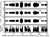 |
Fig. 2. Eleven short bursts of data obtained during a 250 msec interval during the type III emission. Panels a and b give the X and Y components of the electric field in the spacecraft frame. Panel c gives the density fluctuations that are expected to accompany Langmuir waves. Panel d presents the angle in the X − Y plane between the background magnetic field and the electric field wave vector. The largest event, near 11:43:15.460, is discussed in the main text, and the small and medium size events near 11:43:15.450 and 11:43:15.580 are discussed in the appendix. |
In a Langmuir wave, the relation between the density fluctuations and the electric potential is given as Bellan (2006)
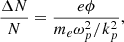
where ϕ is the potential of the wave, kp is the wave number of the wave, and ωp = 2π × 125 kHz is the Langmuir wave frequency. This relation is a direct consequence of the momentum equation and mass-conservation law for electrons. This is the first measurement of the relation between the density fluctuations and the wave potential, although it was studied previously (Neugebauer 1976; Kellogg et al. 1999).
Figure 3a shows the electron velocity distribution function (vdf) during an 80-second interval surrounding the field events of Figure 2, using data obtained from on-board electron measurements (Whittlesey et al. 2020). Because this data collection interval is about 5000 times greater than the duration of Figure 2 and because Langmuir waves only appeared during a small fraction of this time (see Figure 1a), the vdf of Figure 3a is an average over an interval that is largely devoid of Langmuir waves. The currents obtained from the core and strahl distributions are 4.3 and −7.7 microamps/m2.
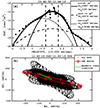 |
Fig. 3. Electron and field properties during the type III event. Panel a gives the electron velocity distribution function during an 80-second interval surrounding the 15-millisecond-long Langmuir wave. It describes the core, halo, and strahl distributions, which show that the average core electron density and thermal velocity were 181 cm−3 and 2887 km/s. Panel b gives the hodogram of the electric field during this event. The hodogram is in the X − Y plane, but because BZ ≈ 0, it describes the relation between the electric field and the magnetic field direction, which is the green line. The electric field is generally parallel to the magnetic field, with significant deviations that are described in Figure 2d. The red curve in Figure 3b represents one period of the wave at the time of the data in Figure 6. |
Figure 3b presents the hodogram of the electric field in the X − Y plane. Because, as noted, Bz ≈ 0, the hodogram illustrates the relation between the electric field k-vector and the magnetic field (the green line in Figure 3b). Figure 3b shows that the electric field was generally parallel to the background magnetic field, with deviations that are described in Figure 2d.
Figure 4 presents spectra of the electric field (black), magnetic field (red), and density fluctuations (green) for the largest event in Figure 2. (Similar results for both a small- and a medium-amplitude event are presented in the appendix). All three quantities in Figure 4 had spectral peaks near the plasma frequency of 125 kHz, with the magnetic field peak previously presumed to result from interaction of the plasma oscillations with ion sound waves to produce Z-mode waves (Gurnett & Anderson 1976; Hospodarsky & Gurnett 1995). At the seven harmonics of the Langmuir frequency, prominent electric fields were observed without measurable magnetic field components. If magnetic fields with amplitudes relative to that at the Langmuir frequency existed, they would be below the noise threshold of the measurement. That these harmonics are real and not artifacts of an imperfect measurement is clear from the fact that if they were not real, there would be no harmonics and no type III emission. Other examples of wave spectra are given in Figures A.1 and B.1.
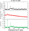 |
Fig. 4. Spectra of the electric field, the magnetic field, and the density fluctuations observed during the intense burst in Figure 2. The lowest frequency wave, at 125 kHz, is at the Langmuir frequency and has both a magnetic and density fluctuation component. Six electric field harmonics of the intense burst are observed, and three of them have detectable density fluctuations. |
That the electric field instrument is capable of measurements at the frequencies observed in Figure 4 is verified from the fact that the time required to change the spacecraft potential by 1 volt through charging its 1 × 10⁻¹⁰ farad capacitance by the photoemission current of about 5 × 10⁻³ amps is about 2 × 10⁻⁸ seconds.
Theories of these harmonic waves that are produced in density cavities (Ergun et al. 2008; Malaspina et al. 2012) do not apply to our observations because density cavities were not present at the times of any of the events discussed on the day of interest. Instead, the harmonics were likely created by a single wave in an electron beam that grew exponentially until the beam electrons were trapped. At this time, the wave amplitude stopped growing and began to oscillate about a mean value. During the trapping process, the beam electrons were bunched in space, and higher harmonics of the electric field were produced (O’neil et al. 1971; O’Neil & Winfrey 1972).
Properties of the electromagnetic waves near the Langmuir frequency may be obtained by considering the ratio of their electric fields to their magnetic fields. For a full field measurement, this gives the phase velocity of the wave. Although only two components of E and one component of B were measured, their ratio can give an estimate of the phase velocity. In Figure 5, this ratio is plotted for the 11 events in Figure 2, and the average velocity thereby obtained is about 50 000 km/s. This is an overestimate of the velocity because part of the electric field was in the electrostatic, not the electromagnetic, wave. With a frequency of 125 kHz, this wave had a wavelength shorter than 400 meters and a k-value greater than 0.015. From the electron core temperature of 23 eV and the plasma density of 181 cm−3, both obtained from the vdf of Figure 3a, the Debye length was 2.65 meters. Thus, kλd was greater than 0.04.
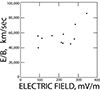 |
Fig. 5. Single component of the electric field divided by a single component of the magnetic field for the 11 events depicted in Figure 2. For a full measurement, this ratio is equal to the phase velocity of the wave. The ratio is an overestimate of the phase velocity of the electromagnetic wave because part of the electric field resulted from an electrostatic wave. Thus, the phase velocity of the electromagnetic wave was < 50 000 km/s. |
The phase velocity of the Langmuir wave may be estimated from equation (1) using the measured electric field of 250 mV/m and the density fluctuations of 0.02 in Figure 2. With the uncertainties in each of these quantities of about a factor of two, the k-value obtained from equation (1) is 0.14. This gives kλd = 0.4 and a phase velocity of the electrostatic wave that was lower than 10 000 km/s.
When a positive electric field in the wave passes over the spacecraft, V1 (which is the potential of antenna 1 minus the spacecraft potential) first becomes positive and then, V2 becomes negative (because the spacecraft potential becomes positive before the antenna potential becomes positive). Their time difference gives the time required for the wave to propagate across the antenna system, which is proportional to the phase velocity of the wave. While the phase velocity of the electrostatic wave can be estimated in this way, this time difference in fact varied over a range so wide that no such measurement was possible. In addition, the ratio of the few volt amplitude of V1 to the amplitude of V2 varied by almost two orders of magnitude, as illustrated in Figure 5a. These facts must be due to the presence of two waves whose amplitudes at each antenna add together to produce the observed wave. However, two waves with constant and different frequencies add to produce beats such as those in Figure 6c, and this is not observed. Because the Langmuir-wave frequency is proportional to the square root of the density, its frequency varied with time as it passed over density irregularities. The density plot of Figure 6b shows that this is an important effect because the density varied by as much as 10% in the vicinity of the observations. Allowing the Langmuir-wave frequency to vary pseudo-randomly by 1 or 2 percent would produce many different curves. A typical such curve is illustrated from a simulation in Figure 6d. Thus, we conclude that the signal near the Langmuir frequency is made of an electromagnetic wave with a phase velocity of about 25 000 km/s and a Langmuir wave whose frequency varied as it passed over density irregularities. As shown in Figure C.1, the harmonics of two other waves each also contained two waves, one of which had a frequency that also varied during its passage over the spacecraft because these variations in the voltage ratio and time delay also occurred in these data.
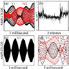 |
Fig. 6. Properties of the single probe potentials. Panel a shows the few-volt potentials on antennas 1 and 2 during a one-millisecond interval. Their difference must be due to the addition of two waves at each antenna, with the Langmuir wave having a variable frequency to avoid the beats produced by two fixed-frequency waves, as illustrated in panel c. The Langmuir-wave frequency varied because of the high-density irregularities illustrated in panel b, to produce a simulation in panel d of the signals on the two antennas that are produced by 1 or 2 percent Langmuir-wave frequency variations. |
It is important to note that the rapid (faster than one millisecond) amplitude variations typical of the Langmuir wave and its harmonics are artifacts resulting from the addition of two waves, and that the observed wave amplitude is not representative of the true wave amplitude versus time.
3. Discussion
The above analyses show that slow electrostatic waves (phase velocity < 10 000 km/s) existed near the Langmuir frequency at as many as six harmonics, the number of which increases with the amplitude of the Langmuir wave. Their electrostatic nature is shown by measurements of density fluctuations of the appropriate magnitudes at each frequency. These harmonics were likely created by a single wave in an electron beam that grew exponentially until the beam electrons were trapped. At this time, the wave amplitude stopped growing and began to oscillate about a mean value. During the trapping process, the beam electrons were bunched in space, and higher harmonics of the electric field were produced (O’neil et al. 1971; O’Neil & Winfrey 1972). The process of the conversion of these harmonics into electromagnetic waves via propagation through an inhomogeneous plasma having density fluctuations is a process was frequently studied (Stix 1965; Oyo 1971; Melrose 1980b, 1981; Mjolhus 1983; Morgan & Gurnett 1990; Kalaee & Ono 2009; Schleyer et al. 2013; Kim et al. 2013; Kalaee & Katoh 2016). It is plausible that the Langmuir frequency harmonics were converted into type III emissions in this way.
We emphasize that none of these results are required of or are explained by the conventional model of the three-wave interaction of two counter-streaming Langmuir waves that coalesce to produce the type III wave. No evidence has been found in this study or earlier studies that requires this coalescence model to be understood.
There is also an electromagnetic wave near the Langmuir frequency with a phase velocity lower than 50 000 km/s. We cannot determine whether there are electromagnetic waves at the harmonics of the Langmuir frequency because if they existed, their magnetic field components would be below the noise level of the measurement. A possible explanation of this wave and the existence of a slow electrostatic wave is given below.
The following discussion of the current-driven generation of electrostatic and electromagnetic fields at frequencies very close to the electron plasma frequency, ωp, is based on the results of previous studies (Sauer & Sydora 2015, 2016; Sauer et al. 2017, 2019) on the excitation of current-driven Langmuir oscillations with ω = ωe and k = 0 by which, subsequently, a parametric decay in Langmuir and ion-acoustic waves with a finite wave number is triggered. We assumed that the electron component is composed of two parts: a dominant population at rest, and a minor component in relative motion, as seen in the core, halo, and strahl of Figure 3. The mechanism of wave excitation does not take into account beam instabilities that may occur in an earlier phase of the interaction. The electron current resulting from the relative motion between the two electron components is crucial for triggering the Langmuir oscillations.
A characteristic electron velocity distribution function of the solar wind is shown in Figure 7a together with the related dispersion of Langmuir waves in the wave number range up to kλd = 0.6. As shown in Figure 7b, due to the occurrence of the electron-acoustic mode that is associated with the strahl, mode splitting takes place at the point where the Langmuir mode of the main population is crossed, that is, at kλd ≈ 0.3. Correspondingly, the related phase velocity is Vph ≈ 3.5Ve (Figure 6b). Around this point the Langmuir or electron-acoustic mode is weakly damped (Figure 7c) and its frequency approaches the plasma frequency, ωp (see the red points). As shown in earlier papers (Sauer & Sydora 2015, 2016; Sauer et al. 2017, 2019), the current due to the strahl drives Langmuir oscillations at ωe, and simultaneously, Langmuir or electron-acoustic waves are driven by parametric decay. Their wave length is given by that of the electron-acoustic mode at ω ≈ ωe, which in our case is kλd ≈ 0.3.
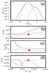 |
Fig. 7. a) Model electron velocity distribution function (EVDF) of the solar wind consisting of the core, halo, and strahl and the associated dispersion of the Langmuir and electron-acoustic mode. b) Frequency ω/ωe, c) phase velocity Vph/Ve, where Ve is the thermal core velocity, and d) damping rate γ/ωe. |
Four arguments supporting the validity of the observed density data are listed below.
-
In other publications, density fluctuations obtained from the spacecraft potential have been observed and shown to be valid at low and high frequencies (Roberts et al. 2020; Mozer et al. 2023). These fluctuations have also been observed in laboratory measurements (Hu et al. 2021).
-
Figure 1c illustrates the Langmuir frequency obtained from the plasma density, which in turn was obtained from the spacecraft potential. That the plasma frequency of Figure 1c agrees with the measured plasma frequency of Figure 1a is proof of the validity of the low-frequency density estimate obtained from the spacecraft potential.
-
Equation (1) presents the theoretical relation between the electric potential (or field) in the wave and the density fluctuations, ΔN/N, that is required in an electrostatic wave. That the ratio of the electric field to ΔN/N in this equation is within a factor of two equal to the more variable measured ratios is evidence that the determination of the density from the spacecraft potential is valid at high frequency.
-
A further requirement of equation (1) is that the electric field and density fluctuation in the high-frequency wave be 90 degrees out of phase. This has been found to be the case (see Figure D.1 in the appendix), which provides conclusive evidence that the electric field and ΔN/N. were well measured and that they were not artifacts of a poor measurement.
Previously observed Langmuir-wave electric fields have ranged from a few to about 100 mV/m (Gurnett & Anderson 1976; Graham & Cairns 2012; Sauer et al. 2017). This range is associated with the range of driving current densities in the plasma. The observed electric field of about 300 mV/m is a factor of three larger than the largest of the previously observed Langmuir waves (Malaspina et al. 2010). The explanation of this difference may lie in the fact that the Langmuir waves had a wavelength that was longer than the three-meter Parker Solar Probe antenna, but was similar to or shorter than the typical antennas that made the earlier measurements. An antenna that is longer than the wavelength of the wave underestimates the amplitude of the true electric field because of the many wavelengths of the field that are inside the antenna. This antenna property may explain why the largest earlier electric field measurements were smaller than observed in the current example.
The rapid (faster than one millisecond) amplitude variations typical of the Langmuir wave and its harmonics are artifacts resulting from the addition of two waves, one of which has small frequency variations that arise from traveling through density irregularities.
Acknowledgments
This work was supported by NASA contract NNN06AA01C. The authors acknowledge the extraordinary contributions of the Parker Solar Probe spacecraft engineering team at the Applied Physics Laboratory at Johns Hopkins University. The FIELDS experiment on the Parker Solar Probe was designed and developed under NASA contract NNN06AA01C. Our sincere thanks to J.W. Bonnell, M. Moncuquet, and P. Harvey for providing data analysis material and for managing the spacecraft commanding and data processing, which have become heavy loads thanks to the complexity of the instruments and the orbit.
References
- Bale, S. D., Goetz, K., Harvey, P. R., et al. 2016, Space Sci. Rev., 204, 49 [Google Scholar]
- Bellan, P. M. 2006, Fundamentals of Plasma Physics (Cambridge University Press) [CrossRef] [Google Scholar]
- Dulk, G. A. 1985, ARA&A, 23, 169 [Google Scholar]
- Ergun, R. E., Malaspina, D. M., Cairns, I. H., et al. 2008, Phys. Rev. Lett., 101, 051101 [NASA ADS] [CrossRef] [Google Scholar]
- Ginzburg, V. L., & Zheleznyakov, V. V. 1958, Sov. Astron., 2, 653 [NASA ADS] [Google Scholar]
- Goldman, M. V., Reiter, G. F., & Nicholson, D. R. 1980, Phys. Fluids, 23, 388 [NASA ADS] [CrossRef] [Google Scholar]
- Graham, B., & Cairns, I. H. 2012, J. Geophys. Res.: Space Phys., 118, 3968 [Google Scholar]
- Gurnett, D. A., & Anderson, R. R. 1976, Science, 194, 1159 [NASA ADS] [CrossRef] [Google Scholar]
- Hospodarsky, G. B., & Gurnett, D. A. 1995, Geophys. Res. Lett., 22, 10 [Google Scholar]
- Hu, Y., Yoo, J., Ji, H., Goodman, A., & Wu, X. 2021, Rev. Sci. Instrum., 92, 033534 [NASA ADS] [CrossRef] [Google Scholar]
- Jebaraj, I. C., Krasnosalskikh, V., Pulupa, M., Magdalenic, J., & Bale, S. D. 2023, ApJ, 955, L20 [NASA ADS] [CrossRef] [Google Scholar]
- Kalaee, M. J., & Katoh, Y. 2016, Phys. Plasmas, 23, 072119 [NASA ADS] [CrossRef] [Google Scholar]
- Kalaee, M. J., Ono, T., Katoh Y., Lizima, M., Nishimura, Y., 2009, Earth Planets Space, 61, 765 [Google Scholar]
- Kellogg, P. J. 1980, ApJ, 236, 696 [NASA ADS] [CrossRef] [Google Scholar]
- Kellogg, P. J., Goetz, K., & Monson, S. J. 1999, J. Geophys. Res., 104, A8 [Google Scholar]
- Kim, E. H., Cairns, I. H., & Johnson, J. R. 2013, Phys. Plasmas, 20, 122103 [NASA ADS] [CrossRef] [Google Scholar]
- Malaspina, D. M., Cairns, I. H., & Ergun, R. E. 2010, J. Geophys. Res., 115, A01101 [NASA ADS] [CrossRef] [Google Scholar]
- Malaspina, D. M., Cairns, I. H., & Ergun, R. E. 2012, ApJ, 755, 45 [NASA ADS] [CrossRef] [Google Scholar]
- Melrose, D. B. 1980a, Space Sci. Rev., 26, 3 [NASA ADS] [CrossRef] [Google Scholar]
- Melrose, D. B. 1980b, Aust. J. Phys., 33, 121 [NASA ADS] [CrossRef] [Google Scholar]
- Melrose, D. B. 1981, J. Geophys. Res.: Space Phys., 86, 30 [NASA ADS] [CrossRef] [Google Scholar]
- Melrose, D. B. 1987, Sol. Phys., 111, 89 [NASA ADS] [CrossRef] [Google Scholar]
- Mjolhus, E. 1983, J. Plasma Phy., 30, 179 [CrossRef] [Google Scholar]
- Morgan, D. D., & Gurnett, D. A. 1990, Radio Sci., 25, 1321 [Google Scholar]
- Mozer, F. S., Bale, S. D., Kellogg, P. J., et al. 2022, ApJ, 926, 220 [NASA ADS] [CrossRef] [Google Scholar]
- Mozer, F. S., Agapitov, O., Bale, S. D., et al. 2023, ApJ, 957, L33 [NASA ADS] [CrossRef] [Google Scholar]
- Neugebauer, M. 1976, Geophys. Res., 81, 78 [NASA ADS] [CrossRef] [Google Scholar]
- O’Neil, T. M., & Winfrey, J. H. 1972, Phys. Fluids, 15, 1514 [CrossRef] [Google Scholar]
- O’neil, T. M., Winfrey, J. H., Malmerg, J. H., et al. 1971, Phys. Fluids, 14, 1204 [CrossRef] [Google Scholar]
- Oyo, H. 1971, Radio Sci., 6, 1131 [NASA ADS] [CrossRef] [Google Scholar]
- Pedersen, A., Cattell, C., Falthammar, C.-G., et al. 1984, Space Sci. Rev., 37, 269 [NASA ADS] [CrossRef] [Google Scholar]
- Reiner, M. J., & MacDowall, R. J. 2019, Sol. Phys., 294, 91 [NASA ADS] [CrossRef] [Google Scholar]
- Roberts, O. W., Nakamura, R., Torkar, K., et al. 2020, J. Geophys. Res. Space Phys., 125, 24 [CrossRef] [Google Scholar]
- Sauer, K., & Sydora, R. 2015, J. Geophys. Res. Space Phys., 120, 235 [NASA ADS] [CrossRef] [Google Scholar]
- Sauer, K., & Sydora, R. 2016, Geophys. Res. Lett., 43, 7348 [NASA ADS] [CrossRef] [Google Scholar]
- Sauer, K., Malaspina, D. M., Pulupa, M., & Salem, C. S. 2017, J. Geophys. Res. Space Phys., 122, 7005 [NASA ADS] [CrossRef] [Google Scholar]
- Sauer, K., Baumgärtel, K., Sydora, R., & Winterhalter, D. 2019, J. Geophys. Res. Space Phys., 124, 68 [NASA ADS] [CrossRef] [Google Scholar]
- Schleyer, F., Cairns, I. H., & Kim, E.-H. 2013, Phys. Plasmas, 20, 032101 [NASA ADS] [CrossRef] [Google Scholar]
- Smith, D. F. 1970, Sol. Phys., 15, 202 [NASA ADS] [CrossRef] [Google Scholar]
- Smith, R. A., Goldstein, M. L., & Papadopoulos, K. 1976, Sol. Phys., 46, 515 [NASA ADS] [CrossRef] [Google Scholar]
- Stix, T. H. 1965, Phys. Rev. Lett., 15, 878 [NASA ADS] [CrossRef] [Google Scholar]
- Sturrock, P. A. 1964, NASA Spec. Pub., 50, 451 [NASA ADS] [Google Scholar]
- Whittlesey, P. L., Berthomier, M., Larson, D. E., et al. 2020, ApJ, 246, 14 [NASA ADS] [Google Scholar]
- Zheleznyakov, V. V., & Zaitsev, V. V. 1970, Sov. Astron., 14, 47 [NASA ADS] [Google Scholar]
Appendix A: Power spectra of a 30 mV/m Langmuir wave
In Figure A.1 the spectra associated with a lower amplitude Langmuir wave are displayed. Although this wave was an order-of-magnitude smaller than the wave having the spectra of Figure 4, the peaks near the plasma frequency and its first harmonic of the electric field of panel A.1(a), the magnetic field of panel A.1(b) and the density fluctuations of panel A.1(c) show that this wave and its harmonic were also slow electrostatic waves.
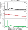 |
Fig. A.1. Spectra of a 30 mV/m Langmuir wave. |
Appendix B: Power spectra of a 150 mV/m Langmuir wave
The wave of Figure B.1 also shows spectral peaks similar to those observed for a 300 mV/m wave (Figure 4) and a 30 mV/m wave (Figure A.1). These same peaks were observed for all waves in Figure 2, so they were typical of the waves observed during the type III emission..
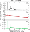 |
Fig. B.1. Spectra of a 150 mV/m Langmuir wave |
Appendix C: Antenna potentials for plasma frequency and first harmonic waves observed at two different times
Figure C.1 illustrates the single-ended potentials V1 and −V2 for the plasma waves of panels C.1(a) and C.1(b) and their first harmonics in panels C.1(c) and C.1(d) at the time of the low amplitude plasma waves in panels C.1(b) and C.1(d) and the medium amplitude plasma waves in panels C.1(a) and C.1(c). Because, in all cases, the ratio of the two potentials varied by large factors, pairs of electrostatic waves existed during both the events with at least one of the pair being slow. This same behavior was observed for all the bursts of Figure 2.
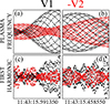 |
Fig. C.1. Single-ended antenna potentials for two wave events. |
Appendix D: Relative timing of the electric field and the density fluctuations
Equation 1 requires that the electric field and density components of a wave be 90 degrees out of phase. This requirement is verified in Figure D.1. which illustrates several cycles of the electric field and density fluctuations near the plasma frequency in panels D.1(a) and D.1(b) and the first harmonic in panels D.1(c) and D.1(d). For each case a vertical dashed line allows comparison of the phase difference between the E-field and the density wave, which is found to be close to 90 degrees. This result supports the conclusion that the waves were accurately measured.
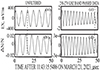 |
Fig. D.1. Relative timing of the electric field and density waves. |
All Figures
|
Fig. 1. Overview of the type III emission observed on March 21, 2023 (panel a) in which the spacecraft was embedded, showing bright lines below the emission due to large electric fields. The plasma frequency of 125 kHz in panel c shows that these bright lines were due to waves at or near the plasma frequency. These waves are present only part of the time. Panel b shows the times and electric field amplitudes of 26 data bursts taken for durations of about 15 milliseconds each at data rates in excess of one million samples/second. |
| In the text | |
|
Fig. 2. Eleven short bursts of data obtained during a 250 msec interval during the type III emission. Panels a and b give the X and Y components of the electric field in the spacecraft frame. Panel c gives the density fluctuations that are expected to accompany Langmuir waves. Panel d presents the angle in the X − Y plane between the background magnetic field and the electric field wave vector. The largest event, near 11:43:15.460, is discussed in the main text, and the small and medium size events near 11:43:15.450 and 11:43:15.580 are discussed in the appendix. |
| In the text | |
|
Fig. 3. Electron and field properties during the type III event. Panel a gives the electron velocity distribution function during an 80-second interval surrounding the 15-millisecond-long Langmuir wave. It describes the core, halo, and strahl distributions, which show that the average core electron density and thermal velocity were 181 cm−3 and 2887 km/s. Panel b gives the hodogram of the electric field during this event. The hodogram is in the X − Y plane, but because BZ ≈ 0, it describes the relation between the electric field and the magnetic field direction, which is the green line. The electric field is generally parallel to the magnetic field, with significant deviations that are described in Figure 2d. The red curve in Figure 3b represents one period of the wave at the time of the data in Figure 6. |
| In the text | |
|
Fig. 4. Spectra of the electric field, the magnetic field, and the density fluctuations observed during the intense burst in Figure 2. The lowest frequency wave, at 125 kHz, is at the Langmuir frequency and has both a magnetic and density fluctuation component. Six electric field harmonics of the intense burst are observed, and three of them have detectable density fluctuations. |
| In the text | |
|
Fig. 5. Single component of the electric field divided by a single component of the magnetic field for the 11 events depicted in Figure 2. For a full measurement, this ratio is equal to the phase velocity of the wave. The ratio is an overestimate of the phase velocity of the electromagnetic wave because part of the electric field resulted from an electrostatic wave. Thus, the phase velocity of the electromagnetic wave was < 50 000 km/s. |
| In the text | |
|
Fig. 6. Properties of the single probe potentials. Panel a shows the few-volt potentials on antennas 1 and 2 during a one-millisecond interval. Their difference must be due to the addition of two waves at each antenna, with the Langmuir wave having a variable frequency to avoid the beats produced by two fixed-frequency waves, as illustrated in panel c. The Langmuir-wave frequency varied because of the high-density irregularities illustrated in panel b, to produce a simulation in panel d of the signals on the two antennas that are produced by 1 or 2 percent Langmuir-wave frequency variations. |
| In the text | |
|
Fig. 7. a) Model electron velocity distribution function (EVDF) of the solar wind consisting of the core, halo, and strahl and the associated dispersion of the Langmuir and electron-acoustic mode. b) Frequency ω/ωe, c) phase velocity Vph/Ve, where Ve is the thermal core velocity, and d) damping rate γ/ωe. |
| In the text | |
|
Fig. A.1. Spectra of a 30 mV/m Langmuir wave. |
| In the text | |
|
Fig. B.1. Spectra of a 150 mV/m Langmuir wave |
| In the text | |
|
Fig. C.1. Single-ended antenna potentials for two wave events. |
| In the text | |
|
Fig. D.1. Relative timing of the electric field and density waves. |
| In the text | |
Current usage metrics show cumulative count of Article Views (full-text article views including HTML views, PDF and ePub downloads, according to the available data) and Abstracts Views on Vision4Press platform.
Data correspond to usage on the plateform after 2015. The current usage metrics is available 48-96 hours after online publication and is updated daily on week days.
Initial download of the metrics may take a while.